The Importance of the Loss Function in Option Valuation

Texte intégral

(1)2003s-52. The Importance of the Loss Function in Option Valuation Peter Christoffersen, Kris Jacobs. Série Scientifique Scientific Series. Montréal Août 2003. © 2003 Peter Christoffersen, Kris Jacobs. Tous droits réservés. All rights reserved. Reproduction partielle permise avec citation du document source, incluant la notice ©. Short sections may be quoted without explicit permission, if full credit, including © notice, is given to the source..

(2) CIRANO Le CIRANO est un organisme sans but lucratif constitué en vertu de la Loi des compagnies du Québec. Le financement de son infrastructure et de ses activités de recherche provient des cotisations de ses organisationsmembres, d’une subvention d’infrastructure du ministère de la Recherche, de la Science et de la Technologie, de même que des subventions et mandats obtenus par ses équipes de recherche. CIRANO is a private non-profit organization incorporated under the Québec Companies Act. Its infrastructure and research activities are funded through fees paid by member organizations, an infrastructure grant from the Ministère de la Recherche, de la Science et de la Technologie, and grants and research mandates obtained by its research teams. Les organisations-partenaires / The Partner Organizations PARTENAIRE MAJEUR . Ministère du développement économique et régional [MDER] PARTENAIRES . Alcan inc. . Axa Canada . Banque du Canada . Banque Laurentienne du Canada . Banque Nationale du Canada . Banque Royale du Canada . Bell Canada . Bombardier . Bourse de Montréal . Développement des ressources humaines Canada [DRHC] . Fédération des caisses Desjardins du Québec . Gaz Métropolitain . Hydro-Québec . Industrie Canada . Ministère des Finances [MF] . Pratt & Whitney Canada Inc. . Raymond Chabot Grant Thornton . Ville de Montréal . École Polytechnique de Montréal . HEC Montréal . Université Concordia . Université de Montréal . Université du Québec à Montréal . Université Laval . Université McGill ASSOCIÉ À : . Institut de Finance Mathématique de Montréal (IFM 2) . Laboratoires universitaires Bell Canada . Réseau de calcul et de modélisation mathématique [RCM 2] . Réseau de centres d’excellence MITACS (Les mathématiques des technologies de l’information et des systèmes complexes) Les cahiers de la série scientifique (CS) visent à rendre accessibles des résultats de recherche effectuée au CIRANO afin de susciter échanges et commentaires. Ces cahiers sont écrits dans le style des publications scientifiques. Les idées et les opinions émises sont sous l’unique responsabilité des auteurs et ne représentent pas nécessairement les positions du CIRANO ou de ses partenaires. This paper presents research carried out at CIRANO and aims at encouraging discussion and comment. The observations and viewpoints expressed are the sole responsibility of the authors. They do not necessarily represent positions of CIRANO or its partners.. ISSN 1198-8177.

(3) The Importance of the Loss Function in Option Valuation* Peter Christoffersen †, Kris Jacobs‡ Résumé / Abstract Quelle devrait être la fonction de perte utilisée pour l’estimation et l’évaluation des modèles de valorisation des options? Plusieurs fonctions ont été suggérées, mais aucune norme ne s’est imposée. Dans ce travail, nous ne proposons pas une fonction en particulier, mais nous soutenons que la cohérence dans le choix des fonctions est cruciale. Premièrement, pour n’importe quel modèle donné, la fonction de perte utilisée dans l’estimation des paramètres et dans l’évaluation du modèle devrait être la même, sinon on obtient des estimations de paramètres sous-optimaux. Deuxièmement, lors de la comparaison des modèles, la fonction de perte utilisée pour l’estimation devrait être la même pour chaque modèle, autrement les comparaisons sont injustes. Nous illustrons l’importance de ces questions dans une application du modèle appelé Black-Scholes du praticien (PBS) aux options de l’indice S&P500. Mots clés : fonctions de volatilité implicite; évaluation des erreurs; prévision hors échantillon; stabilité des paramètres.. Which loss function should be used when estimating and evaluating option valuation models? Many different functions have been suggested, but no standard has emerged. We emphasize that consistency in the choice of loss functions is crucial. First, for any given model, the loss function used in parameter estimation and model evaluation should be the same, otherwise suboptimal parameter estimates may be obtained. Second, when comparing models, the estimation loss function should be identical across models, otherwise inappropriate comparisons will be made. We illustrate the importance of these issues in an application of the so-called Practitioner Black-Scholes model to S&P 500 index options. Keywords: implied volatility functions; valuation errors; out-of-sample forecasting; parameter stability. Codes JEL : G12; G13; C22. *. We would like to thank Torben Andersen, Jeremy Berkowitz, Tim Bollerslev, Michael Brandt, Jerome Detemple, Jin Duan, Rene Garcia, Nour Meddahi, Eric Renault, and seminar participants at Erasmus, the Rotman School, the May 2001 CRDE conference on “Modeling, Estimating, and Forecasting Volatility,” the June 2001 CIRANO conference on “Financial Mathematics and Econometrics,” and the January 2003 Winter Meetings of the Econometric Society for helpful comments. We would also like to thank IFM2 of Montréal, FCAR of Québec, and SSHRC of Canada for financial support. † Corresponding author. Faculty of Management, McGill University, Montreal, Quebec, Canada, H3A 1G5. Tel.: 1-514-398-2869; fax 1-514-398-3876., E-mail address: peter.christoffersen@mcgill.ca. ‡ McGill University, Faculty of Management, Montréal, Canada H3A 1G5; CIRANO, Montréal, Canada, H3A 2A5..

(4) 1. Introduction. The literature on option valuation has expanded dramatically over the last decade. A large number of models have been proposed to address the empirical shortcomings of the classic Black-Scholes (BS) (1973) approach. For instance, an important class of models specifies the volatility of the underlying asset as a deterministic function of time and the price of the underlying asset (see, e.g., Derman and Kani (1994); Dupire (1994); Rubinstein (1994)). Other studies have investigated stochastic volatility models (see, e.g., Scott (1987), Hull and White (1987); Heston (1993); Melino and Turnbull (1990)), jump models (Bates (1996a)), and discrete-time GARCH models (see, e.g., Duan (1995); Heston and Nandi (2000)).1 The objective of this paper is to contribute to the methodological debate on the estimation and evaluation of option valuation models. In particular, we investigate the importance of the loss function. It is well known in the statistics literature that the choice of loss function is critical for model estimation and evaluation. In fact, it can be argued that the choice of loss function implicitly defines the model under consideration (Engle, 1993). Standard theoretical option valuation models imply a deterministic option price and thus do not tell the empirical researcher how to specify the error term (Renault, 1997). The choice of loss function is key because it implicitly assumes a particular error structure. Given the importance of the loss function, it is evident that the estimation and evaluation stages of a model are inextricably linked. Indeed, if the choice of loss function affects the model specification, then estimating a model under one loss and evaluating it under another amounts to changing the model specification without allowing the parameter estimates to adjust. Common sense thus suggests the use of identical loss functions at the estimation and evaluation stages in order to minimize evaluation loss. However, perhaps because the implications of the choice of loss function are less obvious than those of the theoretical model, this common-sense recommendation is often ignored. The choice of loss function is particularly important in option valuation. Option valuation models are rarely estimated to draw inference about a structural parameter of intrinsic interest. Rather, they are typically estimated for use in the valuation or hedging of traded options out-of-sample. Thus different purposes, for example, hedging, speculating, or market making, imply different loss functions for the model errors. We therefore recommend that one uses the objective of the exercise to determine the loss function. Moreover, we postulate that it will generally be preferable to estimate the parameters for such an out-of-sample exercise using an identical in-sample estimation loss function. The existing academic literature has a different focus: to a large extent it ignores the (out-of-sample) evaluation loss function when estimating the parameters. Implicitly this strategy appears to be motivated by the belief that loss functions and model specification 1 For a more complete overview of different approaches used in option pricing, see Bakshi, Cao, and Chen (1997) and Bates (1996b).. 2.

(5) are totally separate from each other. One typically starts with a model that (presumably) performs “well.” Model performance is assumed to be consistent across a wide range of evaluation criteria or loss functions. As a result, the choice of the loss function used in estimation is focused on creating a statistical environment that allows for the most precise and efficient estimation of the parameters of this “good” model. For instance, some papers in the literature advocate a loss function based on implied volatility. Others calibrate and estimate their models using loss functions based on squared dollar pricing errors (see, e.g., Heston and Nandi (2000); Bakshi, Cao, and Chen (1997)), relative pricing errors, or a likelihood-based approach (Jacquier and Jarrow (2000)). We argue that this separation of the estimation and evaluation stages is misguided because the choice of the loss function in the evaluation stage is part of the specification of the statistical model. As this choice depends on the end-use of the model, we do not promote a particular loss function but rather emphasize that consistency in the choice of loss functions is likely to be crucial. Our contribution to the option valuation literature in this regard is threefold: First, we provide evidence that when implementing option valuation models, it is critical to align the estimation and evaluation loss functions. We illustrate the importance of the loss function in an application of the benchmark Dumas, Fleming, and Whaley (DFW) (1998) implied volatility model, which they refer to as the Ad-Hoc model and which we refer to as the Practitioner Black-Scholes (PBS) model. We illustrate our methodological point using the PBS model estimated daily, both because of its simplicity and because of its use as a benchmark in the existing literature. We do not advocate the use of the PBS model over structural models. Instead, we follow Berkowitz (2001), who provides a theoretical justification for the PBS approach as a reduced-form approximation to an unknown structural model, and also provides support for frequent re-estimation of the PBS parameters without necessarily considering the PBS model to be a proper, fully specified alternative to structural models. Using three years’ data of European options on the S&P 500 index, we show that correctly aligning the estimation and evaluation loss functions can yield improvements of over 50% in the evaluation loss and therefore conclude that at least for this type of model, aligning estimation and evaluation loss functions works very well. Second, we emphasize that when comparing models, the estimation loss function should be identical across models otherwise inappropriate comparisons will be made. The PBS model is typically implemented using an implied volatility loss function, which conveniently yields a linear estimator of the parameters. Implemented in this way, the PBS model is easily outperformed by structural stochastic volatility or GARCH option valuation models implemented with an estimation loss function which matches the evaluation loss. Our empirical study shows, however, that when the PBS model is implemented by using the same estimation loss function as that of the structural model, the PBS model actually outperforms the standard structural model both in- and out-of-sample. Third, by implementing the PBS model fairly, we introduce a new PBS model with aligned loss functions, that performs much better than the prior model. This modified PBS model 3.

(6) represents a tougher benchmark against which future structural models can be compared. The paper proceeds as follows. In Section 2, we first discuss the different loss functions used in empirical option valuation and provide an overview of their use in the literature. We then present the Practitioner Black-Scholes approach as implemented by DFW and introduce our modification of their approach. Finally, we briefly summarize the relevant theoretical results on estimation under different loss functions. Section 3 presents our main empirical results and Section 4 compares the PBS model to Heston’s (1993) model and further explores the results. Section 5 conducts various robustness checks and Section 6 concludes.. 2. Methodology. The choice of loss function is particularly important when estimating option valuation models because they have several purposes, for example, hedging, speculating or market making. Different purposes, in turn, naturally suggest different loss functions. Because the specification of a loss function implicitly amounts to the specification of a statistical model (Engle (1993)), one might expect that the choice of loss function would be a hotly debated issue in the option valuation literature. This is not the case. In fact, in the extensive and growing literature on option valuation, the specification of the loss function has not received much attention compared with other issues such as model specification and the estimation of continuous-time processes underlying option models. For example, the excellent literature overview in Campbell, Lo, and MacKinlay (1997) does not list any contributions relating to the importance of the selection of the loss function. Moreover, existing discussions of the loss function in option valuation center on the statistical environment needed to estimate the parameters of a theoretical option valuation model, implicitly ignoring the impact the loss function has on the specification of the statistical model. The unwritten rule seems to be that when the model parameters are “properly” estimated in-sample, they automatically qualify for use in any out-of-sample evaluation exercise, no matter what its objective is. In contrast, we postulate that in most situations, one can minimize out-of-sample loss by using the same loss function in estimation. The motivation for our recommendation is the insight that the choice of the loss function is indeed part of the model specification. Common sense then suggests that one use identical (statistical) models in estimation and evaluation. The use of different loss functions at the estimation and evaluation stages is generally accepted and widely used in the literature. For example, Bakshi, Cao, and Chen (1997) use $MSE in estimation, but %MSE as well as $MSE in the evaluation stage, where $MSE denotes mean-squared absolute option pricing errors and %MSE denotes mean-squared relative option pricing errors. IV MSE stands for mean squared absolute implied volatility error. Rosenberg and Engle (2002) use $MSE in estimation, but % hedging errors in evaluation. Hutchinson, Lo and Poggio (1994) use an MSE-based option price divided by exercise price, yet evaluate the model out-of-sample using hedging errors, among other things. Sev4.

(7) eral papers estimate model parameters from option prices using an estimation loss function based on the statistical properties of the underlying process or the statistical structure of the measurement errors (see, e.g., Renault (1997); Jacquier and Jarrow (2000)) and then proceed to evaluate the models out-of-sample using a different loss function. Pan (2002) uses a generalized method of moments (GMM) loss function in estimation and implied volatility mean squared error, IV MSE, in evaluation. Chernov and Ghysels (2000) estimate parameters using efficient method of moments (EMM), and evaluate models using $MSE and %MSE loss functions. Benzoni (2002) estimates parameters using both EMM and $MSE (normalized by the index value) and proceeds to evaluate the model using $MSE (again normalized). Finally, whereas most recent papers estimate option valuation parameters using option data or option data as well as returns data, until recently many option valuation studies were conducted by estimating option model parameters from asset returns and inserting these parameters into option valuation formulae out-of-sample. Again, this amounts to using different loss functions in-sample and out-of-sample. Problems may arise when one compares out-of-sample errors from misaligned loss functions with errors derived from models where the in-sample and out-of sample loss functions are identical. The statistics literature has pointed out that changing the loss function amounts to changing the model specification (Granger (1969); and Engle (1993)). From this perspective, it is clear that the “correctly specified” model will yield the best in-sample fit, but not necessarily the best out-of-sample fit. Out-of-sample, a misspecified model with precisely estimated parameters may outperform the correctly specified model. No general theorems exist to guide us in this matter, and thus, aligning the estimation and evaluation loss functions serves as a rule-of-thumb. As the usefulness of this rule is an empirical question, we are careful to state that problems may arise, but will not generally occur when loss functions are misaligned. For example, DFW (1998) compare the out-of-sample performance of the PBS model with the out-of-sample performance of deterministic volatility models implemented with identical in- and out-of-sample loss functions. The conclusion of DFW is that the valuation performance of the PBS model compares favorably with that of the deterministic volatility models. Because the implementation of the PBS model proposed in this paper will most likely not deteriorate the model’s performance, the conclusions of DFW will therefore be reinforced when the PBS model is implemented properly. This may not be the case, however, for the studies by Heston and Nandi (2000) and Garcia, Luger, and Renault (2000). Both these papers use the $MSE loss functions for the out-of-sample comparison, but use the implied volatility based loss function for the PBS model in estimation. Heston and Nandi (2000) then compare the PBS model with a GARCH model which has identical in-sample and out-of-sample loss functions. They find that the GARCH model improves upon the performance of the PBS model. Garcia, Luger, and Renault (2000) compare PBS to a new Generalized Black-Scholes model, which is also implemented with aligned loss functions and is also found to dominate the PBS model. The potential problem is that both studies use the PBS model as an evaluation benchmark, but the performance of the 5.

(8) benchmark is not as good as it would be if it were implemented using the appropriate loss function. Note that while these papers do not align the loss functions, it does not mean that the authors are unaware of the limitations of this approach. The papers implement the PBS model as a benchmark, and in doing so they follow the standard practice of estimating the parameters using the implied volatility loss function. We now analyze the impact of the loss function in more detail. First, we describe the loss functions most commonly used to estimate and calibrate parameters in empirical option valuation. Then we introduce the PBS model which can be viewed as an ad-hoc model of the well-known “smile” and “smirk” patterns exhibited by standard derivatives prices. Finally, we discuss how different loss functions imply different model specifications, which in turn motivates the ensuing empirical study.. 2.1. Option model evaluation. The performance of different option valuation models is often evaluated using mean-squared dollar errors; that is, the loss function is given by 1X (Ci − Ci (θ))2 n i=1 n. $MSE(θ) ≡. (1). where Ci and Ci (θ) are the data and model option prices, respectively, and n is the number of option contracts used. Note that although we estimate new parameters each day, we omit the time subscript, t, on the parameters in this section in order to save on notation. The $MSE loss function has the advantage that the errors are easily interpreted as $-errors once the square root is taken of the mean-squared error. However, the relatively wide range of option prices across moneyness and maturity raises the problem of heteroskedasticity for $MSE-based parameter estimation. Also, because the $MSE loss function implicitly assigns a lot of weight to options with high valuations (in-the-money and long time-to-maturity contracts) and therefore high $errors, some researchers instead favor the relative or percent mean-squared error loss function,2 defined as n 1X ((Ci − Ci (θ))/Ci )2 (2) %MSE(θ) ≡ n i=1 where that the %-sign is a convenient short-hand for relative loss. We do not in fact multiply the relative loss by 100, and thus the losses are not expressed in percent but rather decimals. The %MSE loss function has the advantage that a $1 error on a $50 dollar option carries less weight than a $1 error on a $5 option, which is sensible from a rate-of-return perspective. 2 Note that the %-sign below is just a convenient short-hand for relative loss. We do not in fact multiply the relative loss by 100 anywhere, and so the losses are not actually expressed in percent but in decimals.. 6.

(9) The disadvantage is that short time-to-maturity out-of-the money options with valuations close to zero will implicitly get assigned a lot of weight and can thus create numerical instability. Based on the above considerations of heteroskedasticity, and moreover on the market convention of quoting option prices in terms of volatility, some researchers favor estimating option valuation models minimizing the MSE of the implied Black-Scholes volatility from the option. We therefore define the implied volatility MSE as 1X IV MSE(θ) ≡ (σ i − σ i (θ))2 , n i=1 n. (3). where the implied volatilities are σ i = BS −1 (Ci , Ti , Xi , S, r) and σ i (θ) = BS −1 (Ci (θ), Ti , Xi , S, r),. (4). and BS −1 is the inverse of the Black-Scholes formula, Ti the time-to-maturity, Xi the strike price, S the price of the underlying stock, and r the riskless interest rate. This paper only considers the loss functions in (1), (2), and (3). As discussed above, a number of other estimation loss functions are used in the literature. Functions based on hedging or speculation loss could potentially be more interesting, but we focus on the three functions listed here as they are arguably the most prevalent in previous work.. 2.2. The Practitioner Black-Scholes model. We illustrate the importance of the estimation loss function using the simplest model possible, the Practitioner Black-Scholes (PBS) model. In the PBS model, implementation is done in three steps. First the Black-Scholes implied volatility is calculated for each observed option. Second, the implied volatilities are regressed on different polynomials in T and X using simple ordinary least squares (OLS). Third, the fitted values for volatility are plugged back into the Black-Scholes formula to obtain the practitioner model price. DFW consider different implied volatility functions. We limit our attention to the most general model they investigate, which is of the form3 σ = θ0 + θ1 X + θ2 X 2 + θ3 T + θ4 T 2 + θ5 XT + εIV. (5). and where the fitted value of the implied volatility is σ(θ) = θ0 + θ1 X + θ2 X 2 + θ3 T + θ4 T 2 + θ5 XT. 3. (6). DFW consider switching between specifications based on the number of maturities available in their data set on any given day. We use the specification in (5) on all but one day, for which our data set contains only few maturities; on that day we omit the T 2 term.. 7.

(10) Notice that estimating (5) by OLS amounts to letting the estimation loss function be IV MSE. OLS solves 1X (σ i − σ i (θ))2 = (Z 0 Z)−1 Z 0 σ, n i=1 n. θIV = Arg min IV MSE(θ) ≡ Arg min θ. θ. (7). where Z is the matrix of regressors from the implied volatility model. Written in terms of option prices rather than volatilities, the IV MSE loss function implies an error specification of the form C = C BS (σ(θIV ) + εIV ). (8) Thus, the dollar price is a nonlinear function of the IV MSE error term. In order to evaluate the model, the estimate of the parameter vector, θIV , is plugged back into the implied volatility model, which in turn is plugged into the Black-Scholes formula. It is clear from the above equation, however, that simply plugging σ(θIV ) into the Black-Scholes formula will yield a biased estimate of the observed call price. While OLS will ensure that E[εIV ] = 0, the nonlinearity of the dollar option price in volatility and thus in εIV implies that E[C] 6= C BS (σ(θIV )). (9) Ignoring this inequality, the PBS model is typically assessed using. or. n ¢2 1 X¡ Ci − CiBS (σ i (θIV )) $MSE(θIV ) = n i=1. %MSE(θIV ) =. n ¢ ¢2 1 X ¡¡ Ci − CiBS (σ i (θIV )) /Ci n i=1. (10). (11). In the above framework, the estimation loss function, defined on implied volatilities, is different from the evaluation loss function, defined on dollar or percent pricing errors. While this is a convenient and easily implemented procedure, it is inappropriate if the model is assessed in terms of a $MSE or %MSE loss function. If the evaluation loss function is $MSE, the appropriate procedure is to use nonlinear least squares (NLS) to directly estimate θ as follows: n ¢2 1 X¡ θ$ = Arg min $MSE(θ) ≡ Arg min Ci − CiBS (σ i (θ)) . θ n i=1. (12). One way to see the consequences of this choice of evaluation loss function is that implicitly the model under consideration is now C = C BS (σ(θ$ )) + ε$ . 8. (13).

(11) In spite of the fact that the functional form for implied volatility is identical, this model is quite different from the model estimated using the IV MSE loss function, due to the new error structure. Whereas the model estimated in (7) is linear in the parameters the model in (13) is not. The change of loss function corresponds to a nontrivial transformation of the model and the choice of loss function cannot be seen as separate from the choice of model. By choosing an evaluation loss function, one chooses a very important dimension of the specification of the model. This issue has been given some attention in the statistics literature,4 but it is all too often ignored in option valuation applications. The critical impact of the choice of loss function can, of course, also be illustrated in the case of the relative error loss function %MSE. In this case, the model parameters are obtained by solving the following optimization problem n ¢ ¢2 1 X ¡¡ θ% = Arg min %MSE(θ) ≡ Arg min Ci − CiBS (σ i (θ)) /Ci . θ n i=1. (14). Written in terms of dollar option prices, the %MSE loss function implies the following error structure: C = C BS (σ(θ% )) + Cε% . (15) It is clear from comparing (15) with (13) that the choice of the relative error loss function in (14) over the dollar loss function in (12) really amounts to the choice of a different model: the use of the relative error loss function implies a multiplicative heteroskedastic error structure, in contrast to the error structure in (13). It is clear that the three different estimation loss functions implicitly correspond to three different model specifications, even though they are all intended to estimate the parameters of the PBS model (5). Consequently, using an estimation loss function which is different from the evaluation loss will result in suboptimal estimates in terms of evaluation loss. We close this section by noting that we do not promote any particular loss function per se; rather, we stress the importance of being consistent in the choice of loss function. In order to obtain the best possible fit, the loss function used in evaluation should also be used in estimation. Similarly, if a researcher is interested in comparing several models, care should be taken that the estimation loss function is identical across models, otherwise inappropriate comparisons will be made. 4. See, for example, Granger (1969), Weiss and Andersen (1984), Engle (1993), and Weiss (1996). For an option pricing application see Garcia and Gencay (2000).. 9.

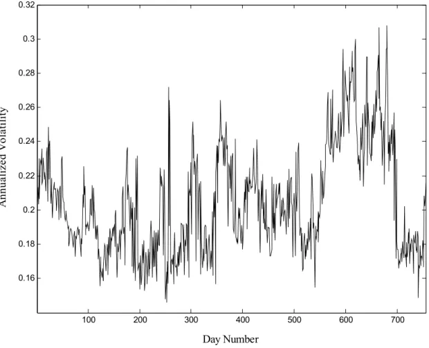
(12) 3 3.1. Empirical results Data. We analyze the methodological issues outlined above using a very standard data set, namely the S&P 500 call option prices on 755 days in the period from June 1, 1988 through May 31, 1991. The data were graciously provided to us by Gurdip Bakshi and are practically identical to the data used in Bakshi, Cao, and Chen (1997). We limit ourselves here to a few important features of the data and refer the reader to their study for further details. The data set is well suited for our empirical analysis because options written on the S&P 500 are the most actively traded European-style contracts. Particular care is taken to adjust the S&P 500 spot index series for dividend payments and to obtain synchronous recording of stock and option prices. The resulting data set contains a wide variety of option quotes for different values of moneyness and maturity. Table 1, Panel A lists the number of contracts for a set of maturity and moneyness bins, where S/X denotes the option’s moneyness and DT M stands for days to maturity. To be exact, we are sorting the data by (S − Di )/Xi , where Di is the present value of dividends accruing to option i until its expiration. Table 1, Panel B reports the average price for option contracts with different moneyness and maturities. For our purpose, the most important observation in Table 1, Panel B is the large difference in option prices across maturities and moneyness; expensive contracts will implicitly receive much more weight in the $MSE loss function than cheap contracts. In Table 1, Panel C we report the average implied Black-Scholes volatilities from the call prices in Table 1, Panel B. Notice that in general the implied volatilities are much less variable across entries in the table than are the call prices themselves. Notice also that the well-known post-crash smirk is apparent in every column, but that it is most apparent at the shortest maturity. As mentioned above, we investigate the importance of the choice of loss function by estimating the relevant parameters for each of the 755 daily cross-sections. Figure 1 indicates that the optimization problem under study can be substantially different for different days. To illustrate the variation over the sample, we depict the average Black-Scholes implied volatility calculated on each of the 755 days in the sample. Notice that implied volatility changes through time but that swings in average implied volatility seem to be relatively persistent across time. This finding suggests that the out-of-sample performance of the daily models may actually turn out to be fairly satisfactory if the parameters are appropriately estimated.. 3.2. Empirical loss estimates. The main results of the paper are contained in Figures 2.A-2.B and in Table 2. For each day in the sample we repeat the following exercise. First, we estimate the parameter θ 10.

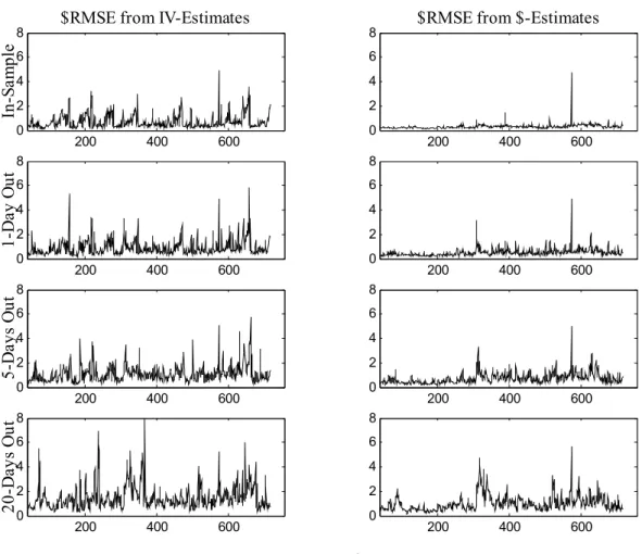
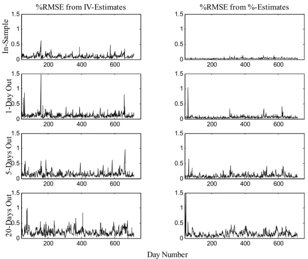
(13) characterizing the implied volatility function in (5) using three different loss functions. We refer to these three estimates of θ as θt,$ , θt,% , and θt,IV , , respectively, where the t subscript indicates that the estimate is obtained using the t-th day (or cross-section) in the sample. The first estimate, θt,$ , is obtained by minimizing the $MSE loss function in (1). The second estimate, θt,% , is obtained by minimizing the %MSE loss function (2). The third estimate, θt,IV , is obtained by minimizing the IV MSE loss function in (3). We then use these estimates to evaluate the model’s valuation performance in- and out-of-sample for different loss functions. This exercise is similar to Dumas, Fleming and Whaley (1998). Brandt and Wu (2002) and Hull and Suo (2002), on the other hand, investigate the usefulness of the PBS model fitted to standard European options in-sample for pricing other options out-ofsample.5 Possibly the most interesting exercise is to evaluate the different loss functions one day out-of-sample. Consider the second row of pictures in Figure 2.A. These pictures show the square root of MSEs (RMSE) for the dollar-based loss function (1) evaluated at t + 1 using parameter estimates obtained at t. In the left panel the estimate used is θt,IV , which is obtained by minimizing the “wrong” loss function (3). In contrast, in the right panel, the estimate θt,$ is obtained by minimizing the “correct” loss function (1). The differences in RMSE between the two panels are striking. While on a few occasions (especially in the second half of the sample) the RMSE is quite large in the right panel, it is often minuscule when compared to its analog in the left panel. The other panels in Figure 2.A contain results for related exercises. In the two top panels we present the same exercise using estimates θt,IV and θt,$ , but with the RMSE computed for the same day t (in-sample). Again we observe that the RMSE in the left panel is much larger than in the right panel. The third and fourth row of panels again use the estimates θt,IV and θt,$ , but now the RMSE is evaluated at days t + 5 and t + 20, respectively, corresponding roughly to one-week and one-month ahead. While the deterioration in loss is obvious for both sets of estimates as the horizon lengthens, the $-estimates appear to clearly outperform the IV-estimates even at the 20-day horizon. Figure 2.B presents results for an exercise that is analogous to the one presented in Figure 2.A, except that the RMSEs are now calculated from the percentage-based loss function (2) evaluated at t, t + 1, t + 5, and t + 20. The estimates used correspond to those obtained from the “wrong” loss function θt,IV and the “correct” loss function θt,% . The conclusion from Figure 2.B is identical to that obtained from Figure 2.A: the use of the wrong loss function in estimation leads to dramatic underperformance in the in-sample and out-of-sample RMSE. Table 2 summarizes the information in Figures 2.A and 2.B by presenting the average 5. Our data set contains one day (day 348) with only few available contracts at longer maturities. Following Dumas, Fleming and Whaley (1998), on that day we exclude the squared maturity term from the implied volatility polynomial. Including the squared maturity term on that day results in unusual parameter estimates, but it changes the quantitative loss estimates only marginally and does not change any of our qualitative conclusions.. 11.

(14) RMSE computed over the 716 days in the prediction sample. In Figures 2.A and 2.B and in Table 2, we omit the first 39 observations in order to conduct out-of-sample analysis and to ensure comparability with results in later tables, which use longer estimation samples. Consider first the leftmost three columns labelled “Raw Loss.” The diagonal in each part of the table corresponds to the loss from using the relevant loss function in estimation. Off-diagonal entries report the losses from using estimates that minimize a loss function different from the relevant one. For example, for the results in Figure 2.A, we look in the second column. We see that on average, when using the appropriate loss function to obtain the estimates θt,$ , the one-day out-of-sample RMSE is 0.4901, whereas if the wrong loss function is used to obtain θt,IV , the average RMSE is 0.8708. For 5-days out-of-sample, the corresponding RMSEs are 0.6864 and 1.0510, respectively. Even at the 20-day horizon, the RMSEs are quite different at 1.4373 and 0.9760, respectively. The data in Figure 2.B is summarized in the third column, where again, we see large average improvements in RMSEs from using the appropriate loss function. Finally, in the left column we present evidence on an estimation exercise not reported in Figure 2. While most studies cited above use the dollar-based loss function (1) or percentage-based loss function (2) for out-of-sample performance evaluation, we investigate which average RMSEs one would obtain when evaluating the square root of the IV MSE (3) out-of-sample. It can be seen that at t, t + 1, or t + 5, we obtain the lowest RMSEs by using the appropriate in-sample loss function, but at t + 20 the $-estimates actually slightly outperform the IV-estimates even when using the IV RMSE metric. Notice also that the differences across estimates in IV RMSE loss are generally much smaller than the differences across estimates in $RMSE and %RMSE loss. In order to facilitate the comparison of different RMSEs, the rightmost three columns of Table 2 report the average RMSEs from before, divided by the RMSE from the relevant loss function. Notice that except for the IV RMSE loss at t + 20, the relative loss is always at least one. Notice also that the IV estimates fare particularly poorly when used in the other loss functions. These tables therefore illustrate our main point that it is important to use the relevant loss function. As a rule of thumb, researchers should be consistent in their choice: the estimation loss function should be the same as the evaluation loss function. Even though some loss functions have obvious econometric problems associated with them, such as heteroskedasticity and numerical stability issues, our analysis indicates that these concerns are generally outweighed by the gains from matching loss functions. However, our results suggest that a researcher indifferent on the choice of loss function may prefer the $MSE loss function.. 12.

(15) 4 4.1. Exploring the results Comparison with a structural model. So far the empirical analysis has focused on documenting the improvement in the evaluation loss when the appropriate estimation loss is used. We now ask if the loss function issue is important enough to reverse existing empirical rankings of models. Interestingly, it is. To document this, we compare the PBS model’s valuation performance with the valuation performance of the classic stochastic volatility model proposed by Heston (1993). Heston’s model assumes that the stock price under risk neutrality evolves according to p dS(t) = rSdt + v(t)Sdz1 (t) (16). with the variance process. dv(t) = κ(ϕ − v(t))dt + σ. p v(t)dz2 (t),. (17). where dz1 (t) and dz2 (t) are standard Brownian motions with correlation coefficient ρ. It is well-known from a number of recent papers that the empirical performance of this model is not entirely satisfactory and that extending the model can improve its pricing performance (see Andersen, Benzoni, and Lund (2002); Bakshi, Cao, and Chen (1997); Benzoni (2002); Chernov and Ghysels (2000); Jones (2001, 2002); Pan (2002)). Here, we simply want to compare different applications of the PBS model to a mainstream structural model that is easy to implement and which fits the data reasonably well. The Heston model is attractive because it yields an analytical solution for the option price (up to a numerical integral that can be evaluated quickly and accurately). This solution can be found in Heston (1993) and Bakshi, Cao, and Chen (1997). We implement this model by estimating the four parameters κ, ϕ, σ, and ρ. Also, because we estimate the model on a day-by-day basis, we follow the example of Bakshi, Cao, and Chen (1997) and estimate the initial conditional volatility, v(0), as a fifth parameter each day. However, we estimate these parameters for all three loss functions, $MSE, %MSE, and IV MSE. We then proceed to evaluate the model insample and out-of-sample and to compare the pricing errors with those of the PBS model. The daily re-estimation approach is inconsistent with the theory, which assumes that the parameters are constant over time. We choose this approach to bring the implementation of the structural model as close as possible to that of the PBS model. The same approach is taken in Bakshi, Cao, and Chen (1997). To evaluate the model, the expected future variance is calculated as Et [v(t + τ )] = ϕ + e−κτ [v(t) − ϕ] , (18) where τ is the forecast horizon. Table 3 presents average RMSE losses for the Heston model using the same 716 days of options contracts that are used to generate the empirical results in Table 2. To facilitate 13.

(16) comparisons between the models, in Table 3 we repeat certain entries from Table 2. Certain contracts have been removed due to problems inverting some of the Heston model prices when using the IV MSE estimation loss function. To ensure internal comparability within Table 3, these contracts are removed in all cells and as a result, the numbers in Table 3 are not exactly the same as the numbers in Table 2. They are very similar, however. The inversion problems are worst at the 20-day forecast horizon, which therefore has been omitted from Table 3. More detailed evidence on the day-by-day performance of the Heston model is reported in Figure 3. Table 3 clearly illustrates that the use of the appropriate loss function is of critical importance. For instance, consider the performance of the Heston model when the $RMSE loss function is used (Panel B). For the in-sample evaluation the average $RMSE over 716 days is 0.3838 (middle column). Compare this with the PBS model as implemented in DFW (left column). We might conclude that the Heston model beats the benchmark PBS model, because 0.3838 is lower than 0.6642. However, when the PBS model is implemented using the appropriate loss function (right column), the average $RMSE is 0.2923. Therefore, the structural model actually does not perform better than the PBS model when estimated using the relevant loss function. Notice that while the Heston model nests the original BlackScholes (1973) model, it does not nest the PBS model. Therefore, it is possible for the PBS model to have a better fit than the Heston model. If we inspect the $RMSE loss functions evaluated out-of-sample, we see that the average 1-day and 5-day out-of-sample $RMSEs are 0.5727 and 0.8173, higher than 0.4864 and 0.6811, respectively, for the PBS model estimated using $MSE. If we instead use the standard IV MSE-implementation of the model, we would conclude that 0.5727 and 0.8173 are lower than 0.8406 and 1.0124, respectively. Inspection of Table 3, Panel C shows that identical conclusions obtain when we evaluate %RMSE loss functions. For the in-sample evaluation, the average Heston %RMSE of 0.0363 is lower than 0.0958 but higher than 0.0309. For the 1-day out-of-sample exercise, the average Heston %RMSE of 0.0650 is lower than 0.1184 but higher than 0.0597. Finally, for the 5-day out-of-sample exercise, the average Heston %RMSE of 0.1062 is lower than 0.1439 but higher than 0.0935. For completeness, we include in Table 3, Panel A, the Heston (1993) model estimated using the IV MSE loss function. In this case, the standard PBS model implementation corresponds to using the relevant estimation loss function and the left and right columns are therefore identical in this case. Notice that, again, the PBS model performs slightly better than the Heston model when both are estimated and evaluated using the IV RMSE metric. In summary, the conclusions from the comparison of the Heston model with the PBS model are robust. Regardless of whether one uses $RMSE or %RMSE loss functions, and regardless of whether one evaluates the loss functions in-sample or out-of-sample, the PBS model performs better than the Heston model when implemented using the appropriate loss function. However, when the PBS model is implemented using the IV MSE loss function to 14.

(17) estimate the parameters, as is standard in the literature, it performs much worse than the Heston model. When both models are estimated and evaluated using the IV RMSE metric, the PBS model also slightly outperforms the Heston model. We close this section by re-emphasizing that these findings by no means indicate that the PBS model is superior to structural models. The PBS model is an ad-hoc curve-fitting technique and lacks the theoretical and intuitive background of structural models. In particular, structural models provide the key link between the dynamics of the option price and the dynamics of the underlying asset price. The improvement in fit relative to a structural model therefore only indicates its usefulness as a benchmark, and, therefore, does not qualify it as a genuine competitor to structural models.. 4.2. Mincer-Zarnowitz decomposition. Is it possible to provide some intuition for why the IV MSE-based estimates seem so much worse than the $-based and %-based estimates as seen in Tables 2 and 3? Figures 4.A and 4.B graph the estimates of the coefficients in the PBS implied volatility relation (5) for all 755 days. The panels on the left use the IV loss function (3), the panels in the middle use the $-based loss function (1), and the panels on the right use the percentage loss function (2). The problem with the IV MSE estimates for the PBS model seems to be that, although they are obtained from linear regression, they are much more volatile than the estimates from the other loss functions obtained using nonlinear estimation. This parameter variability, evident in Figure 4, may provide an intuitive explanation for the results in Table 2, which, in turn, indicates that the out-of-sample performance of the $-estimates is relatively good while that of the IV estimates is relatively poor. Table 4 attempts to expand on the parameter variability explanation. For the $MSE loss function, we follow Karolyi (1993) and calculate the Mincer-Zarnowitz (1969) decomposition of the MSE into bias-squared, inefficiency, and random variation for the PBS and Heston models. In general we have ¢ ¡ MSE = [E[y] − E[ˆ y ]]2 + (1 − β)2 V ar(ˆ (19) y ) + 1 − R2 V ar(y), where y is the variable of interest and yˆ is its forecast. From the regression of y on yˆ and a constant, we obtain the slope coefficient, β, and the regression fit, R2 . For a given option valuation model we have the $MSE decomposition h i2 ¡ ¢ ˆ + 1 − R2 V ar(C), ˆ = E[C] − E[C(λ)] ˆ + (1 − β)2 V ar(C(λ)) (20) $MSE(λ). ˆ is the model price calculated from a vector where C is the observed market price and C(λ) ˆ We run the Mincer-Zarnowitz regressions on each day for the of parameter estimates, λ. two models and for the in-sample as well as 1-, 5-, and 20-day out-of-sample forecasts. 15.

(18) Table 4 reports the average MSEs and their decompositions across days 40 through 755 of the sample. Note that in order to highlight the decompositions, we report MSEs and not RMSEs, in contrast with earlier tables. The four left columns of Table 4 show the Mincer-Zarnowitz decomposition of the $MSE loss from the Heston model and the rightmost four columns show the decomposition of the PBS model. Naturally, most of the in-sample $MSE arises from random variation. As the forecast horizon increases, bias becomes an increasingly important factor, probably arising from systematic changes in overall market volatility which is not captured in the static models considered here. The contribution to $MSE from inefficiency for the IV estimates is surprisingly modest. Indeed, the majority of the difference in $MSE across the three sets of estimates appears to be random variation. From the perspective of the $MSE loss, the large variation in the IV parameter estimates does not translate into excessive variation in the forecasted option prices. These results hold for the PBS as well as Heston model. Notice also that contrary to what one might expect, the Heston model does not reduce the bias compared to the PBS model even 20-days out. This could of course be due to the implementation of the model; following Bakshi, Cao, and Chen (1997), the parameters including the spot volatility are re-estimated daily.. 5. Robustness checks. The main conclusion from Table 2 is that there are generally large gains to be had from matching the estimation loss function and evaluation loss functions. In this section we perform two types of checks to assess the robustness of this finding. First, to check the effect on our results of the option valuation function shifting over time, we conduct a “same-day out-of-sample” experiment. Second, to check the effect of the relatively small daily estimation samples, we extend the rolling samples to five days and twenty days , respectively. We also perform (not reported here) a third robustness experiment relying on Derman (1999), who models implied volatility in terms of moneyness and maturity rather than strike price and maturity. We implement Derman’s model in a manner identical to the implementation of the DFW specification in Table 2. The Derman model leads to the same qualitative conclusions as the DFW model.. 5.1. Jackknife estimation. From the Mincer-Zarnowitz analysis in Table 4, it is apparent that as the forecast horizon lengthens, the bias increases, presumably due to systematic changes in latent variables. As the PBS model considered here is completely static, a relevant question to ask is whether the key empirical findings in Table 2 will hold in an out-of-sample experiment in which changes in latent variables do not play a role. 16.

(19) In order to answer this question we run the following experiment, which we refer to as Jackknife estimation, borrowing a well-known term from statistics. The PBS model is estimated separately for each contract using only the remaining contracts on the same day. The coefficients are again estimated using the three different estimation loss functions, $MSE, %MSE, and IV MSE. Each set of estimates is used to calculate the evaluation error only of the contract omitted from that particular estimation sample. Table 5 shows the results. The columns under the Raw Loss heading report the daily average RMSE across days 40 through 755. The numbers in the Relative Loss columns have been divided by the diagonal elements where the estimation and evaluation loss functions coincide. The main result here is that matching the estimation and evaluation loss functions generates the lowest loss in each case. This confirms our earlier findings. As expected, the RMSEs are all higher than the in-sample raw loss RMSEs in Table 2. When we compare Table 5 RMSEs with those in the 1-day out raw loss panel of Table 2, we see that the $-estimates and %-estimates generate Jackknife losses that are lower than the RMSEs in Table 2. The IV estimates, on the other hand, generate Jackknife $RMSE and IV RMSE losses which are more comparable to the 5-day out-of-sample RMSEs. This corroborates our second finding, that the IV estimates perform relatively poorly overall. The IV estimates are highly variable and suffer greatly from the estimation sample being reduced by one observation in the Jackknife estimation. The Jacknife losses, which are same-day out-of-sample losses, are generally lower when the estimation and evaluation loss functions coincide. We therefore conclude that the benefits from matching loss functions do not arise only from ignoring changes over time in the underlying state variables.. 5.2. Extending the estimation sample. The deterioration in the loss associated with the IV estimates when one contract is excluded raises the question of the degree to which our empirical findings are due to the relatively small size of the samples used in estimation. While daily re-estimation of the model using only one day of data has the advantage that we can pick up time-variation of the optionvaluation relationship, this benefit may come at the cost of imprecision in the parameter estimates. To address this concern, we repeat the daily analysis of the PBS model in Table 2, but use rolling 5- and 20-day estimation samples instead of rolling 1-day samples. Table 6 shows the results from estimating the PBS model daily using the current and most recent four days’ data and our three different estimation loss functions. Each set of estimates is used to evaluate the daily root mean-squared error (RMSE) loss for the three loss functions. Losses are calculated on the last day of each estimation sample (in-sample) as well as 1-, 5-, and 20-days out-of-sample. The Raw Loss columns report the daily average RMSE across days 40 through 755. The numbers in the Relative Loss columns have been divided by the diagonal elements, where the estimation and evaluation loss functions coincide. 17.

(20) The main result again is that matching the estimation and evaluation loss functions is usually optimal. As before, the only exception is the slightly lower IV RMSE loss for the $-estimates at the 20-day horizon. Table 6 also confirms that, when used in another loss function, the $-based estimates tend to perform relatively better than the IV-based estimates. Notice also that due to the larger estimation sample, the in-sample RMSEs are higher in Table 6 than in Table 2. This deterioration in in-sample fit can be seen as an indication of the quantitative importance of daily parameter re-estimation. Table 7 repeats the experiment of Table 6 using rolling 20-day estimation samples. While the quantitative results change marginally, the qualitative conclusions remain the same.. 6. Conclusions. This paper raises an important methodological question regarding the estimation of parameters for use in option valuation models. Until now, the literature has mainly focused on the choice of a theoretical option valuation model. Once the theoretical model is chosen, the main concern is largely the efficient econometric estimation of the parameters characterizing the model. While there is concern in the literature about the role of the loss function in these estimation procedures, the application of the loss function in the evaluation stage is little more than an afterthought. We argue that the relevant discussion should not start out by discussing how to estimate the parameters, but rather by stating what functional form the evaluation (typically out-of-sample) loss function takes. The specification of the loss function is dictated by the purpose of the empirical exercise, for instance, it may be related to a hedging problem or a risky investment strategy. It may be difficult at first to intuitively grasp why this specification issue is of more than philosophical importance. The key is that one should stop thinking of the specification of a theoretical model as separate from the choice of the loss function. When operationalizing a deterministic theoretical model, whether for estimation or evaluation purposes, one has to impose a statistical structure. This statistical structure is an integral part of empirical model specification, and the choice of loss function is a major part of the statistical structure. Our recommendation, to align the estimation and evaluation loss functions, differs from existing practice, which focuses on the efficient estimation of a set of parameters regardless of the loss function used when evaluating the model. The paper demonstrates that our recommendation works very well in practice. This is illustrated by focusing on the simplest model available in the literature that attempts to account for the well-known biases in the Black-Scholes model, namely, the Practitioner BlackScholes (PBS) model. The PBS model is typically implemented with an estimation loss function that different from the evaluation loss function. Our analysis shows that this procedure generates a problem that is quantitatively important, with the implementation used in the literature leading to out-of-sample RMSEs that are more than twice the lowest-possible 18.

(21) RMSE using the proper estimation loss function. This finding has serious implications both for future studies and papers that have implemented PBS in the traditional way. To demonstrate these implications, we compare the empirical performance of the PBS model to the performance of the well-known stochastic volatility model in Heston (1993). We find that when the PBS model is implemented using an inappropriate loss function, the PBS model performs much worse than the Heston model. However, the PBS model performs somewhat better than the Heston model when the appropriate loss function is used. Thus, our modified PBS model represents a new and tougher benchmark against which the performance of future structural models can be measured. At a more general level, the results in this paper have implications for any situation in which the loss function can be identified. For example, our results suggest that the best possible parameter estimates for a hedging exercise will likely be obtained using a hedgingbased loss function, whereas a speculator would optimally obtain parameter estimates using a loss function consistent with the objective of speculation. In future work, we will investigate these application oriented loss functions, which differ from the statistical ones used in this paper. It must also be noted in this respect that the most appropriate option valuation model to be used for such purposes is probably not the PBS model, but a structural model. The PBS model is used in this paper as an example, because its simplicity facilitates the communication of our message. For many more realistic exercises, a structural model designed to keep parameters constant across time may be more appropriate. An important reason for this is that the loss function for a speculator or a market-maker often involves illiquid contracts such as exotic derivatives; in such situations it is necessary to use structural models that allow for extrapolation across contracts or time, rather than an ad-hoc model, which by its very nature requires frequent re-calibration using liquid contracts. For certain purposes it may not be possible to identify the relevant loss function. In this case, our results indicate that the $MSE estimates perform the best across different loss functions. The $MSE may thus serve as a good general-purpose loss function in option valuation applications. Finally, we stress that when one compares different models, the estimation loss function should be the same otherwise unfair comparisons will be made.. 19.

(22) References [1] Ait-Sahalia, Y., Lo, A., 1998. Nonparametric estimation of state-price densities implicit in financial asset prices. Journal of Finance 53, 499-547. [2] Andersen, T., Benzoni, L., Lund, J., 2002. An empirical investigation of continuous-time equity return models. Journal of Finance 57, 1239-1284. [3] Bakshi, C., Cao, C., Chen, Z., 1997. Empirical performance of alternative option pricing models. Journal of Finance 52, 2003-2049. [4] Bates, D., 1996a. Jumps and stochastic volatility: Exchange rate processes implicit in Deutschemark options. Review of Financial Studies 9, 69-107. [5] Bates, D., 1996b. Testing option pricing models. In; G.S. Maddala, C.R. Rao (Eds.), Handbook of Statistics, Vol 15: Statistical Methods in Finance. North-Holland, Amsterdam, 567-611. [6] Benzoni, L., 2002. Pricing options under stochastic volatility: An empirical investigation. Unpublished working paper. University of Minnesota. [7] Berkowitz, J., 2001. Forecasting option prices with unobserved volatility and false models. Unpublished working paper. University of Houston. [8] Brandt, M., Wu, T., 2002. Cross-sectional tests of deterministic volatility functions. Journal of Empirical Finance 9, 525-550. [9] Black, F., Scholes, M., 1973. The pricing of options and corporate liabilities. Journal of Political Economy 81, 637-659. [10] Campbell, J., Lo, A., MacKinlay, C., 1997. The Econometrics of Financial Markets. Princeton University Press. [11] Chernov, M., Ghysels, E., 2000. A study towards a unified approach to the joint estimation of objective and risk neutral measures for the purpose of option valuation. Journal of Financial Economics 56, 407-458. [12] Derman, E. 1999., Regimes of volatility. Risk 4, 55-59. [13] Derman, E., Kani, I., 1994. Riding on the smile. Risk 7, 32-39. [14] Duan, J., 1995. The GARCH option pricing model. Mathematical Finance 5, 13-32. [15] Dumas, B., Fleming, F., Whaley, R., 1998. Implied volatility functions: Empirical tests. Journal of Finance 53, 2059-2106. 20.

(23) [16] Dupire, B. 1994. Pricing with a smile. Risk 7, 18-20. [17] Engle, R. 1993. A comment on Hendry and Clements on the limitations of comparing mean square forecast errors. Journal of Forecasting 12, 642-644. [18] Garcia, R., Gencay, R. 2000. Pricing and hedging derivative securities with neural networks and a homogeneity hint. Journal of Econometrics 94, 93-115. [19] Garcia, R., Luger, R., Renault, E. 2000. Empirical assessment of an intertemporal option pricing model with latent variables. Unpublished working paper. Universite de Montreal. [20] Granger, C. 1969. Prediction with a generalized cost of error function. Operations Research Quarterly 20, 199-207. [21] Heston, S. 1993. A closed-form solution for options with stochastic volatility with applications to bond and currency options. Review of Financial Studies 6, 327-343. [22] Heston, S., Nandi, S. 2000. A closed-form GARCH option pricing model. Review of Financial Studies 13, 585-626. [23] Hull, J., White, A. 1987. The pricing of options on assets with stochastic volatilities. Journal of Finance 42, 281-300. [24] Hull, J., Suo, W. 2002. A methodology for assessing model risk and its application to the implied volatility function model. Journal of Financial and Quantitative Analysis 37, 297-318. [25] Hutchinson, J., Lo, A., Poggio, T. 1994. A nonparametric approach to pricing and hedging derivative securities via learning networks. Journal of Finance 49, 851-889. [26] Jacquier, E., Jarrow, R. 2000. Bayesian analysis of contingent claim model error. Journal of Econometrics 94, 145-180. [27] Jones, C. 2002. The dynamics of stochastic volatility: Evidence from underlying and options markets. Journal of Econometrics. Forthcoming. [28] Jones, C. 2001. A nonlinear analysis of S&P 500 index option returns. Unpublished working paper. University of Rochester. [29] Karolyi, A. 1993. A Bayesian approach to modeling stock return volatility for option valuation. Journal of Financial and Quantitative Analysis 28, 579-594. [30] Melino, A., Turnbull, S. 1990. Pricing foreign currency options with stochastic volatility. Journal of Econometrics 45, 239-265. 21.

(24) [31] Mincer, J., Zarnowitz, V. 1969. The evaluation of economic forecasts. In: J. Mincer, Zarnowitz, V. (Eds.), Economic Forecasts and Expectations. Columbia University Press, New York. [32] Nandi, S. 1998. How important is the correlation between returns and volatility in a stochastic volatility model? Empirical evidence from pricing and hedging in the S&P 500 index options market. Journal of Banking and Finance 22, 589-610. [33] Pan, J. 2002. The jump-risk premia implicit in options: Evidence from an integrated time-series study. Journal of Financial Economics 63, 3—50. [34] Renault, E. 1997. Econometric models of option pricing errors. In: Kreps, D., Wallis, K. (Eds.), Advances in Economics and Econometrics. Seventh World Congress. Cambridge University Press, New York and Melbourne, pp. 223-278. [35] Rosenberg, J., Engle, R. 2002. Empirical pricing kernels. Journal of Financial Economics 64, 341-372. [36] Rubinstein, M. 1994. Implied binomial trees. Journal of Finance 49, 771-818. [37] Scott, L. 1987. Option pricing when the variance changes randomly: Theory, estimators, and applications. Journal of Financial and Quantitative Analysis 22, 419-438. [38] Weiss, A. 1996. Estimating time series models using the relevant loss function. Journal of Applied Econometrics 11, 539-560. [39] Weiss, A., Andersen, A. 1984. Estimating time series models using the relevant forecast evaluation criterion. Journal of the Royal Statistical Society, Series A 147, 484-487.. 22.

(25) Table 1 The option data are tabulated in moneyness and maturity bins. We use daily closing prices of European call options written on the S&P 500 index. The sample starts on June 1, 1988 and ends on May 31, 1991 for a total of 755 days. DTM denotes days to maturity and S/X denotes moneyness defined as the S&P 500 index value over the option strike price.. Panel A. Number of call option contracts DTM < 60 60<DTM<180 S/X < .94 674 3,075 .94 < S/X < .97 2,058 2,049 .97 < S/X < 1.00 2,604 1,978 1.00 < S/X < 1.03 2,445 1,744 1.03 < S/X < 1.06 2,206 1,501 1.06 < S/X 4,661 4,734 Total 14,648 15,081. 180 < DTM 2,552 1,014 963 803 731 2,690 8,753. Total 6,301 5,121 5,545 4,992 4,438 12,085 38,482. Panel B. Average call price DTM < 60 S/X < .94 1.53 .94 < S/X < .97 2.60 .97 < S/X < 1.00 5.29 1.00 < S/X < 1.03 11.02 1.03 < S/X < 1.06 18.44 1.06 < S/X 39.55 All 18.58. 60<DTM<180 5.09 9.58 14.87 21.25 28.06 49.85 25.19. 180 < DTM 10.30 18.81 25.00 31.32 37.19 62.41 33.09. All 6.82 8.60 12.13 17.86 24.78 48.67 24.47. Panel C. Average implied volatility from call options 60<DTM<180 DTM < 60 S/X < .94 0.1792 0.1719 .94 < S/X < .97 0.1664 0.1719 .97 < S/X < 1.00 0.1713 0.1820 1.00 < S/X < 1.03 0.1899 0.1936 1.03 < S/X < 1.06 0.2161 0.2038 1.06 < S/X 0.3120 0.2349 All 0.2256 0.1987. 180 < DTM 0.1676 0.1767 0.1854 0.1966 0.1950 0.2178 0.1910. All 0.1709 0.1707 0.1775 0.1923 0.2085 0.2608 0.2072. 23.

(26) Table 2 Implied Black-Scholes volatility is modelled as a second-order polynomial in the strike price and years-to-maturity (the PBS model). The coefficients in the polynomial are estimated on each day of the data set using three different estimation loss functions: mean-squared error (MSE) of implied volatility (IV), MSE of dollar prices ($), and MSE of relative prices (%). Each set of estimates is used to evaluate the daily root mean-squared error (RMSE) loss from the three loss functions. Losses are calculated using the estimates in-sample as well as 1-, 5-, and 20-days out-of-sample. The Raw Loss columns report the daily average RMSE across days 40 through 755. The IVRMSE and %RMSE are reported in decimals and $RMSE in dollars. The numbers in the Relative Loss columns have been divided by the diagonal elements, where the estimation and evaluation loss functions coincide.. Raw loss $RMSE. %RMSE. 0.6809 0.2937 0.5448. 0.0970 0.0608 0.0308. 1.0000 1.6782 2.0096. 2.3179 1.0000 1.8546. 3.1469 1.9707 1.0000. Panel B. 1-day out IV estimates 0.0269 $-estimates 0.0314 %-estimates 0.0358. 0.8708 0.4901 0.6820. 0.1208 0.0762 0.0603. 1.0000 1.1698 1.3339. 1.7766 1.0000 1.3915. 2.0038 1.2648 1.0000. Panel C. 5-days out IV estimates 0.0322 $-estimates 0.0340 %-estimates 0.0382. 1.0510 0.6864 0.8467. 0.1473 0.1051 0.0936. 1.0000 1.0571 1.1872. 1.5313 1.0000 1.2336. 1.5749 1.1238 1.0000. Panel D. 20-days out IV estimates 0.0413 $-estimates 0.0391 %-estimates 0.0423. 1.4373 0.9760 1.1061. 0.2022 0.1480 0.1435. 1.0000 0.9474 1.0248. 1.4727 1.0000 1.1333. 1.4084 1.0308 1.0000. IVRMSE Panel A. In-sample IV estimates 0.0163 $-estimates 0.0273 %-estimates 0.0327. 24. Relative loss IVRMSE $RMSE %RMSE.

(27) Table 3 Heston’s stochastic volatility model is estimated daily using three different estimation loss functions: mean-squared error (MSE) of implied volatility (IV), MSE of dollar prices ($), and MSE of relative prices (%). Each set of estimates is used to evaluate the daily root meansquared error (RMSE) loss from the matching estimation loss function. Average RMSE losses are calculated across days using the estimates in-sample, as well as 1- and 5-days out-of-sample. The losses from the Heston model (middle column) are compared with losses from the PBS model using the IV estimates (left column) as well as using the matching loss function estimates (right column). The IVRMSE and %RMSE are reported in decimals and $RMSE in dollars. Certain contracts are omitted due to difficulties in inverting the Heston model prices.. PBS IV-estimates. Heston PBS Matching estimates Matching estimates. Panel A. IVRMSE loss In-sample 1-day out 5-days out. IV-estimates 0.0155 0.0248 0.0293. IV-estimates 0.0176 0.0252 0.0297. IV-estimates 0.0155 0.0248 0.0293. IV-estimates 0.6642 0.8406 1.0124. $-estimates 0.3838 0.5727 0.8173. $-estimates 0.2923 0.4864 0.6811. IV-estimates 0.0958 0.1184 0.1439. %-estimates 0.0363 0.0650 0.1062. %-estimates 0.0309 0.0597 0.0935. Panel B. $RMSE loss In-sample 1-day out 5-days out Panel C. %RMSE loss In-sample 1-day out 5-days out. 25.

(28) Table 4 The parameters in the Heston and PBS models are estimated daily using three different estimation loss functions: mean-squared error (MSE) of implied volatility (IV), MSE of dollar prices ($), and MSE of relative prices (%). For the $MSE loss function we can calculate the Mincer-Zarnowitz decomposition of the MSE into bias squared, inefficiency, and random variation from MSE = [E[y] − E[ˆ y ]]2 + (1 − β)2 V ar(ˆ y ) + (1 − R2 ) V ar(y), where y is the variable of interest and yˆ is its forecast. From the regression of y on yˆ and a constant, we obtain the slope coefficient β and the regression fit R2 . The Mincer-Zarnowitz regressions are run on each day, for each of the three sets of estimates and for the in-sample as well as 1-, 5- and 20-days out-of-sample forecasts. The table reports the average MSEs and their decompositions across days 40 through 755 of the sample.. $-loss Heston model MSE Bias Efficiency Random Panel A. In sample IV estimates 0.6545 0.0185 0.0818 0.5541 $-estimates 0.2113 0.0037 0.0118 0.1957 %-estimates 0.3980 0.0244 0.0547 0.3189. 0.7408 0.1282 0.3822. 0.0021 0.0026 0.0079. 0.0112 0.0017 0.0835. 0.7275 0.1238 0.2908. Panel B. 1-day out IV estimates 1.1633 $-estimates 0.5034 %-estimates 0.6954. 0.1928 0.1578 0.1842. 0.1743 0.0331 0.0966. 0.7962 0.3125 0.4145. 1.0556 0.3353 0.6103. 0.1386 0.1269 0.1270. 0.0366 0.0151 0.1119. 0.8804 0.1933 0.3714. Panel C. 5-days out IV estimates 2.2392 $-estimates 1.0727 %-estimates 1.2927. 0.5987 0.5293 0.6192. 0.3311 0.0509 0.1035. 1.3094 0.4925 0.5699. 1.4149 0.6503 0.9277. 0.3436 0.3309 0.3234. 0.0647 0.0349 0.1367. 1.0066 0.2845 0.4676. Panel D. 20-days out IV estimates 6.8906 $-estimates 2.7728 %-estimates 3.0073. 1.7791 1.4723 1.7719. 1.0217 0.1044 0.1335. 4.0898 1.1962 1.1018. 2.8368 1.3503 1.6676. 0.8377 0.8123 0.7768. 0.1564 0.0808 0.2011. 1.8426 0.4572 0.6897. 26. MSE. $-loss PBS model Bias Efficiency Random.

(29) Table 5 The PBS model is estimated for each contract using only information on the remaining contracts on that particular day. The coefficients are estimated using three different estimation loss functions: mean-squared error (MSE) of implied volatility (IV), MSE of dollar prices ($), and MSE of relative prices (%). Each set of estimates is used to evaluate the daily root mean-squared error (RMSE) loss of the omitted contracts. The Raw Loss columns report the daily average RMSE across days 40 through 755. The IVRMSE and %RMSE are reported in decimals and $RMSE is in dollars. The numbers in the Relative Loss columns have been divided by the diagonal elements, where the estimation and evaluation loss functions coincide.. IV estimates $-estimates %-estimates. IVRMSE 0.0213 0.0281 0.0336. Raw loss $RMSE 1.0497 0.3672 0.6379. %RMSE 0.1408 0.0699 0.0509. 27. IVRMSE 1.0000 1.3190 1.5760. Relative loss $RMSE 2.8590 1.0000 1.7374. %RMSE 2.7661 1.3722 1.0000.

(30) Table 6 The PBS model is estimated daily using the current and four past days of data and using three different estimation loss functions: mean-squared error (MSE) of implied volatility (IV), MSE of dollar prices ($), and MSE of relative prices (%). Each set of estimates is used to evaluate the daily root mean-squared error (RMSE) loss for the three loss functions. Losses are calculated on the last day of each estimation sample (in-sample) as well as 1-, 5and 20-days out-of-sample. The Raw Loss columns report the daily average RMSE across days 40 through 755. The IVRMSE and %RMSE are reported in decimals and $RMSE in dollars. The numbers in the Relative Loss columns have been divided by the diagonal elements, where the estimation and evaluation loss functions coincide.. Relative loss IVRMSE $RMSE %RMSE. Raw loss $RMSE. %RMSE. 0.8582 0.4378 0.6491. 0.1187 0.0733 0.0531. 1.0000 1.3019 1.5329. 1.9604 1.0000 1.4829. 2.2345 1.3790 1.0000. Panel B. 1-day out IV estimates 0.0264 $-estimates 0.0316 %-estimates 0.0368. 0.9291 0.5150 0.7099. 0.1296 0.0822 0.0666. 1.0000 1.1938 1.3903. 1.8042 1.0000 1.3785. 1.9452 1.2334 1.0000. Panel C. 5-days out IV estimates 0.0314 $-estimates 0.0338 %-estimates 0.0385. 1.1240 0.6708 0.8366. 0.1589 0.1056 0.0941. 1.0000 1.0752 1.2268. 1.6756 1.0000 1.2471. 1.6887 1.1226 1.0000. Panel D. 20-days out IV estimates 0.0401 $-estimates 0.0385 %-estimates 0.0420. 1.4604 0.9396 1.0593. 0.2076 0.1467 0.1362. 1.0000 0.9609 1.0479. 1.5543 1.0000 1.1274. 1.5235 1.0766 1.0000. IVRMSE Panel A. In sample IV estimates 0.0233 $-estimates 0.0303 %-estimates 0.0357. 28.

(31) Table 7 The PBS model is estimated daily using the current and nineteen past days of data and using three different estimation loss functions: Mean Squared Error (MSE) of implied volatility (IV), MSE of dollar prices ($), and MSE of relative prices (%). Each set of estimates is used to evaluate the daily root mean squared error (RMSE) loss for the three loss functions. Losses are calculated on the last day of each estimation sample (in sample) as well as 1-, 5and 20-days out-of-sample. The Raw Loss columns report the daily average RMSE across day 40 through 755. IVRMSE and %RMSE are reported in decimals and $RMSE in dollars. The numbers in the Relative Loss columns have been divided by the diagonal elements where the estimation and evaluation loss functions coincide.. Relative loss IVRMSE $RMSE %RMSE. Raw loss $RMSE. %RMSE. 1.0782 0.6059 0.7925. 0.1524 0.0961 0.0800. 1.0000 1.1234 1.3172. 1.7795 1.0000 1.3079. 1.9037 1.2011 1.0000. Panel B. 1-day out IV estimates 0.0310 $-estimates 0.0339 %-estimates 0.0395. 1.1175 0.6393 0.8185. 0.1580 0.1006 0.0860. 1.0000 1.0953 1.2767. 1.7479 1.0000 1.2802. 1.8367 1.1688 1.0000. Panel C. 5-days out IV estimates 0.0338 $-estimates 0.0354 %-estimates 0.0407. 1.2289 0.7332 0.8968. 0.1746 0.1145 0.1027. 1.0000 1.0461 1.2022. 1.6760 1.0000 1.2231. 1.7004 1.1155 1.0000. Panel D. 20-days out IV estimates 0.0394 $-estimates 0.0391 %-estimates 0.0433. 1.5107 0.9316 1.0632. 0.2223 0.1466 0.1356. 1.0000 0.9923 1.0996. 1.6217 1.0000 1.1413. 1.6395 1.0810 1.0000. IVRMSE Panel A. In sample IV estimates 0.0297 $-estimates 0.0334 %-estimates 0.0391. 29.

(32) 0.32. 0.3. Annualized Volatility. 0.28. 0.26. 0.24. 0.22. 0.2. 0.18. 0.16. 100. 200. 300. 400. 500. 600. 700. Day Number. Fig. 1. The average implied Black-Scholes volatility across contracts is plotted for each of the 755 days in the sample. We use daily closing prices of European call options written on the S&P 500 index. The sample starts on June 1, 1988 and ends on May 31, 1991.. 30.