Montréal Mai/May 2014
© 2014 Claudia Keser, Andreas Markstädter. Tous droits réservés. All rights reserved. Reproduction partielle permise avec citation du document source, incluant la notice ©.
Short sections may be quoted without explicit permission, if full credit, including © notice, is given to the source.
Série Scientifique
Scientific Series
2014s-30
Informational Asymmetries in Laboratory Asset
Markets with State-Dependent Fundamentals
CIRANO
Le CIRANO est un organisme sans but lucratif constitué en vertu de la Loi des compagnies du Québec. Le financement de son infrastructure et de ses activités de recherche provient des cotisations de ses organisations-membres, d’une subvention d’infrastructure du Ministère de l'Enseignement supérieur, de la Recherche, de la Science et de la Technologie, de même que des subventions et mandats obtenus par ses équipes de recherche.
CIRANO is a private non-profit organization incorporated under the Québec Companies Act. Its infrastructure and research activities are funded through fees paid by member organizations, an infrastructure grant from the Ministère de l'Enseignement supérieur, de la Recherche, de la Science et de la Technologie, and grants and research mandates obtained by its research teams.
Les partenaires du CIRANO Partenaire majeur
Ministère de l'Enseignement supérieur, de la Recherche, de la Science et de la Technologie
Partenaires corporatifs
Autorité des marchés financiers Banque de développement du Canada Banque du Canada
Banque Laurentienne du Canada Banque Nationale du Canada Banque Scotia
Bell Canada
BMO Groupe financier
Caisse de dépôt et placement du Québec Fédération des caisses Desjardins du Québec Financière Sun Life, Québec
Gaz Métro Hydro-Québec Industrie Canada Intact
Investissements PSP
Ministère des Finances et de l’Économie Power Corporation du Canada
Rio Tinto Alcan Transat A.T. Ville de Montréal
Partenaires universitaires
École Polytechnique de Montréal École de technologie supérieure (ÉTS) HEC Montréal
Institut national de la recherche scientifique (INRS) McGill University
Université Concordia Université de Montréal Université de Sherbrooke Université du Québec
Université du Québec à Montréal Université Laval
Le CIRANO collabore avec de nombreux centres et chaires de recherche universitaires dont on peut consulter la liste sur son site web.
ISSN 2292-0838 (en ligne)
Les cahiers de la série scientifique (CS) visent à rendre accessibles des résultats de recherche effectuée au CIRANO afin de susciter échanges et commentaires. Ces cahiers sont écrits dans le style des publications scientifiques. Les idées et les opinions émises sont sous l’unique responsabilité des auteurs et ne représentent pas nécessairement les positions du CIRANO ou de ses partenaires.
This paper presents research carried out at CIRANO and aims at encouraging discussion and comment. The observations and viewpoints expressed are the sole responsibility of the authors. They do not necessarily represent positions of CIRANO or its partners.
Informational Asymmetries in Laboratory Asset Markets
with State-Dependent Fundamentals
Claudia Keser
*, Andreas Markstädter
†Résumé/abstract
We investigate the formation of market prices in a new experimental setting involving multi-period call-auction asset markets with state-dependent fundamentals. We are particularly interested in two informational aspects: (1) the role of traders who are informed about the true state and/or (2) the impact of the provision of Bayesian updates of the assets’ state-dependent fundamental values (BFVs) to all traders. We find that bubbles are a rare phenomenon in all of our treatments. Markets with asymmetrically informed traders exhibit smaller price deviations from fundamentals than markets without informed traders. The provision of BFVs has little to no effect. Behavior of informed and uninformed traders differs in early periods but converges over time. On average, uninformed traders offer lower (higher) limit prices and hold less (more) assets than informed traders in “good”-state (“bad”-state) markets. Informed traders earn superior profits.
Mots clés/keywords : Experimental economics, asset markets, informational
asymmetries
Codes JEL : C92, D47, D53, D82, G14
*
Corresponding author: Chair of Microeconomics, Faculty of Economic Sciences, Georg-August-Universität Göttingen, E-mail: claudia.keser@uni-goettingen.de; Tel.: +49 (0) 551 - 39 80 40
† Chair of Microeconomics, Faculty of Economic Sciences, Georg-August-Universität Göttingen, E-mail:
2
1. Introduction
Financial markets are characterized by pronounced informational asymmetries. This is particularly true in times of market uncertainty, for example, following economic turbulences or in the wake of stock market launches (IPOs). In order that markets can perform their allocative function under this premise, market prices should reflect all available information. In other words, markets have to be informationally efficient. Assuming market participants to use all available public and private information, the transfer of information considerably influences allocative market efficiency (Leland and Pyle 1977). It is thus crucial to understand to what extent information is revealed through market prices. Ultimately, market prices should be consistent with rational expectations (as defined by Muth 1961) about future benefits and not be driven by informational “mirages”1, speculation or the lack of proper investment alternatives.
With respect to these issues regarding informational asymmetries, the potential influence that insider trading exerts on market prices, unmonitored by financial market authorities, is of particular interest. Apart the fact that unrestricted insider trading is prohibited by law in all prominent financial markets, it likely takes place. Interestingly, Bris (2005), using acquisition data from 52 countries between 1990 and 2000, finds that the introduction of laws that prohibit insider trading increases the occurrence and profitability of insider trading. Jeng et al. (2003), using Center for Research in Securities Prices (CRSP) transactions data from 1975 to 1996, find further that insider purchases yield returns that are more than 6% above expected returns per year, while insider sales do not yield significant abnormal returns. In the ongoing debate between proponents and opponents of deregulation of insider trading in the economic and law literature, to date, neither efficiency nor fairness and equity arguments can mutually persuade the debating parties (Fishman and Hagerty 1992, Bainbridge 1998).
In this paper, we study asset price formation in a new experimental setting involving multi-period assets in an environment with uncertainty about market fundamentals. Specifically, we consider the existence of two possible states of nature. We compare price formation in markets with and without informational asymmetry. In the latter markets, some of the traders do have information on the true state, while other traders don’t. We use the experimental-economics laboratory as a wind channel to study whether financial markets are informationally efficient and how informational asymmetries (due to insider information) impact market price formation. This would hardly be possible (if not impossible) to disentangle on real market grounds, due to the blurry nature of underlying securities’ values and the uncontrollable and incalculable information distribution among market participants in real-life markets. In the experiment we can control the information available to market participants and the
1 Camerer and Weigelt (1991) define mirages in the following way: “[I]n inferring information from the
trades of others, traders sometimes err and their errors cause others to overreact, creating price paths that falsely reveal information that no one has.” (p. 489)
3
securities’ fundamentals. Although the expectation formation of market participants remains difficult to grasp,2 we can explicitly control the informational asymmetries
between market participants, including the number of informed participants (henceforth also inside traders or insiders) relative to the uninformed (henceforth also outside traders or outsiders). We neither claim nor aim to resolve the debate between proponents and opponents of insider trading regulation, however, strive to fuel the discussion with the provision of additional experimental evidence.
Since the seminal paper by Smith et al. (1988) (henceforth, SSW) countless studies have investigated common stock valuation in experimental asset markets with multi-period assets characterized by declining fundamental values (FVs). However, relatively few studies consider informational asymmetries. If (experimental) markets are efficient, the market value should equal the risk-adjusted present value of the rationally expected future financial benefits conditioned on all available information. Asset price changes should only occur when new information is brought into the market, which changes expectations about the income stream (Shiller 2003). Deviations from fundamentals, if at all, should be only temporary until the risk-adjusted expectations converge. Such kind of markets would approximate what Fama (1970), the originator of the efficient-market hypothesis (EMH), called “efficient”. However, SSW-type markets predominantly resist showing efficiency and persistently exhibit bubbles, which hardly can be explained by differences in preferences or risk aversion. The observed bubble-and-crash phenomenon is found to be strikingly robust to changes in the experimental environment.3 “Smart money”4 seems not as smart as desired by theory in view of the
numerously observed experimental (and real-life) bubbles. The only factor that fairly reliably impairs this widely observed pattern is experience (in the sense of repetition). Dufwenberg et al. (2005) have shown that even a fraction of experienced subjects in an experimental market is sufficient to reduce the occurrence of bubbles. However, this seems to hold only if the market environment (initial endowments and dividend structure) remains unchanged during the trials (Hussam et al. 2008).
On the basis of Dufwenberg et al. (2005), Sutter et al. (2012) hypothesize that, in addition to experience, an asymmetric distribution of information about an asset’s imminent future dividends among the participants might serve to reduce mispricing, i.e., the magnitude of bubbles. They argue that the core of this alleviating effect might lie in the common knowledge of the existence of better informed or experienced traders.
2 How the available information disseminates through the market and is processed by the individual
traders to build individual expectations remains a tremendous source of uncertainty. It resembles Keynes (1936) view of the stock market as a “beauty contest” in which traders are more concerned about the beliefs of others than about their own valuation based upon all available information. As good as the experimenters can control for the market parameters, as bad they can control the endogenous beliefs of participants about other participants’ behavior (Noussair and Plott 2008).
3 See, e.g., King et al. (1993), Porter and Smith (1994), or Palan (2009) for comprehensive and salient
reviews of the experimental “bubble” literature. For an overview of bubble definitions see, e.g., Siegel (2003).
4 “Smart money” theory as a branch of the efficient market hypothesis was considered to be able to keep
4
Implementing a SSW framework, they find information asymmetries to significantly reduce the size of price bubbles, implying higher market efficiency. Moreover, they do not detect a significant difference in profits between traders with different information levels. However, in an earlier study, King (1991) finds no evidence for asymmetric distribution of information to eliminate price bubbles in a SSW environment. In his study informed traders, likewise, could not capitalize their informational advantage through higher profits; they were just able to recoup the costs for the acquisition of the private information.5
Another experimental literature strand studies asymmetric information using an approach different from SSW. It is based on one-period Arrow-Debreu assets with state-contingent and trader-type dependent dividends, and in the cases where insider information is investigated, asymmetric distributions of state information (e.g., (Forsythe et al. 1982, Plott and Sunder 1982, Forsythe et al. 1984, Ang and Schwarz 1985, Plott and Sunder 1988, Camerer and Weigelt 1991, Sunder 1992, Friedman 1993, Ackert et al. 1997, Ackert and Church 1998). The studies in this literature strand focus on the test of the “prior information equilibrium pricing prediction model” (PI) versus the “fully revealing rational-expectations equilibrium prediction model” (RE). Both prediction models will be explained in more detail in Section 3 below. In summary, this literature strand shows that markets are generally able to aggregate information quite successfully. PI predictions seem to be a good benchmark for trades in early periods, whereas the RE predictions appear more accurate in later periods. Plott and Sunder (1988), for example, argue as follows: “Rational expectations can be seen either as a static theory of markets (e.g., as in the efficient market literature in finance) or as an end-point of a dynamic path of adjustment.” (p. 1104)
Our experiment is novel in that it combines both literature strands and introduces state-dependence in the SSW framework. In our new framework, insider information is defined as the knowledge of the state. The aim of our study is to analyze how informational aspects, including the existence of inside knowledge, influence price formation and market performance.
In our experiment, the dividend paid by an asset, in each of 15 periods, has four possible values and is the same for all traders. However, in each period, the dividend is stochastic and its distribution function depends upon one of two possible states of the world. In other words, the state determines the probabilities with which the respective dividends are drawn. The “state of the world” is determined at the beginning of the experiment and stays the same over all periods. Traders generally do not know the state but are informed that the probability of each state is 50 percent. This is the prior belief, which determines the ex-ante expected fundamental value of the assets. Based on the observed dividends during the experiment, this belief can be updated according to the method of Bayes, resulting in ex-post expected fundamental values (BFVs) of the assets. In some of
5 Unlike the work of Sutter et al. (2012), which uses randomly assigned and free private information, King
5
the experimental markets informational asymmetry is established via a random assignment of cost-free information about the state to some inside traders.
We investigate how information is processed and disseminated trough market prices. We are particularly interested in two informational aspects: (1) the role of traders who are informed about the true state (insiders), and/or (2) the impact of the provision of Bayesian updates of the assets’ state-dependent fundamental value to all traders. We compare the outcomes in markets where two traders with insider information about the actual “state of the world” are present (and the presence is common knowledge) to the outcomes in markets without any insider information. Additionally, in half of the markets with insiders and half of the markets without insiders, we provide all traders in every period with updated BFVs. In all four resulting treatments, to scrutinize traders’ ability to anticipate uncertain future outcomes, a key issue in financial markets, we elicit traders’ expectations about the future market prices at the beginning of each period and provide monetary incentives for the accuracy of their predictions.
Our main results are the following: We find bubbles to occur rarely in all treatments, even though all traders are inexperienced, i.e., never participated in market experiments before. Markets with asymmetrically informed traders exhibit smaller price deviations from fundamentals, suggesting higher market efficiency. The provision of BFVs has little to no effect. Behavior of in- and outsiders differs in early periods but converges over the course of the markets. On average, we find outsider limit buy/sell prices to be lower (higher) in the “good” (“bad”) state and outsiders to hold less (more) assets in “good”-state (“bad”-“good”-state) markets compared to insiders. Insiders manage to exploit their superior position and are able to earn higher profits. With regard to price expectations, we find forecasts and actual market prices to be highly correlated. Forecast precision, however, seems to be impeded by the presence of insiders, while the provision of BFVs seems to have no impact on forecast quality.
The remainder of this paper is structured as follows: Section 2 presents the experimental market design and describes the experimental procedures. Section 3 introduces two behavioral models and provides testable hypotheses. Section 4 reviews these hypotheses in the face of the results of the experimental markets. Section 5 gives a summary and concludes.
6
2. Laboratory Markets and Experimental Procedures
We conducted the computerized experiment in the Göttingen Laboratory of Behavioral Economics at the University of Göttingen, Germany, based on the z-tree software package (Fischbacher 2007).
A total of 192 subjects participated in 32 markets with six traders, each. Participants were student volunteers recruited for a decision-making experiment via ORSEE (Greiner 2004). All participants were Bachelor or Master Students in business administration or international economics at the University of Göttingen and thus had some background in economics.
Each subject assumed the role of a trader in an asset market. Six participants (henceforth traders) participated in a market lasting 15 periods. Each experiment session involved two or three independent markets. At no time, traders did know the identity of other traders in the market. A market lasted 15 periods and involved trading in call auctions (for buying and selling) in each period.
The experimental sessions were conducted in two parts. In the first part, risk preferences were elicited using lottery choices following Holt and Laury (2002) (see Appendix A for more details). Trading in the call-auction market took place in the second part. For both parts traders were given detailed written instructions. For the first part, written instructions were individually provided. For the second part, instructions were read aloud in a briefing room and supplemented by a presentation of screenshots which included all screens traders encountered during the experiment. Instructions and screenshots of the program are provided in the Appendix C. The whole process before the call-auction market started lasted on average about 45 minutes. During the entire session traders were not allowed to talk to each other.
2.1. Characteristics Common to All Sessions
At the beginning of each experimental market each trader is endowed with 10 assets and 10,000 ECU working capital. We have chosen to provide the same endowment to all traders to prevent trading merely due to the desire to realign portfolios. King et al. (1993) found no significant effect of equal endowments on bubble formation. Each trader’s initial endowment in ECU is large enough to buy at least a quarter of the other traders’ assets in a market at initial fundamental values. Short selling is not permitted. The initial working capital has to be repaid at the end of the market session. Traders’ asset and working capital holdings are carried over from one period to the next.
Prior to the trading stage, at the beginning of each period, traders have to state their expectations about the prospective market prices of the present and all subsequent
7
trading periods. Thus, each trader has to state in each period 𝑡 ∈ (1, … , 15) a total of (16 − 𝑡) forecasts. To create an incentive for participants to care about forecast precision, participants are rewarded (in ECU) for the accuracy of each forecast.6 If the
forecasted price is within a 10 percent, 10-20 percent or 20-30 percent range, a respective reward of 5 ECU, 2 ECU or 1 ECU is paid. For less accurate forecasts no reward is paid. Over the course of the 15 market periods, for any period 𝑡 (1 ≤ 𝑡 ≤ 15) 𝑡 predictions are requested and thus a reward may be obtained up to 𝑡 times. In each period, after all traders have stated their predictions, trading commenced in a call-auction market.
Each of the 15 market periods on average lasted five minutes (including forecasts). In each period, assets with an initial lifetime of 15 periods can be traded. Each asset pays the same dividend to all its holders in a market. The dividend is randomly drawn after the trading at the end of each period. It can take a value of 10 ECU, 20 ECU 40 ECU, or 80 ECU. The fundamental value of an asset is determined by the dividend stream that it generates to its holder. It corresponds to the sum of all expected future dividends. Consequently, the fundamental value declines to zero in the course of a market. After the final payment of the dividend in the last period, the asset becomes worthless.
Since our research focus lies in the propensity of markets to aggregate and disseminate information, we incorporate state-dependency of assets, as in Camerer and Weigelt (1991). Like in the SSW type markets, the dividend from holding an asset does not differ across traders. That means that markets have only one “type” of trader with regard to dividend value. However, the expected dividend depends upon the “state of the world”, which is randomly drawn at the beginning of a market. There are two equally likely states. State 1 is called the “good” and State 2 the “bad” state. The set of possible dividend values is equal in both states of the world but dividend values occur with different probabilities. We have chosen probability distributions of the dividends in order to focus the subjects’ attention on the two different expected values for the “good” and “bad” state and to determine two clearly distinguishable states of the world. Actual dividends originate from independent random draws out of the set {10, 20, 40, 80} of possible dividends. The expected dividend per period in a given state is given by the probability weighted sum of the possible dividends. Table 1 provides the possible per period dividend values and the corresponding probabilities of occurrence under each of the two states. It also provides the expected per period dividend 𝐸𝐷𝑆 in each state 𝑆 ∈
(1, 2).
6 We use incentivized belief elicitation because it can be expected that participants exert more effort to
forecast correctly and that these forecasts are more accurate than non-incentivized, as was, for example, found by Gächter and Renner (2010).
8
Table 1: Possible Dividend Values and Probabilities Possible
Dividends “Good” State (𝑆 = 1) Probability in “Bad” State (𝑆 = 2) Probability in
10 0.1 0.4
20 0.2 0.3
40 0.3 0.2
80 0.4 0.1
𝐸𝐷𝑆 49 26
In the “good” state the probabilities of the higher dividends are larger than in the “bad” state, resulting in a higher expected dividend value per period and a higher FV in each period. The expected dividend per period is 49 in the “good” state and 26 in the “bad'” state. In the first period, with no information about the state at hand the expected dividend is 37.5. This value changes after each period’s dividend draw according to Bayes' theorem, since the updated probability to be in one state or the other also changes according to this rule. For a given “state of the world”, the FV is given by the product of the expected dividend per period and the number of remaining periods the dividend is paid. Formally, the FV in State 𝑆 and period 𝑡 is given by (16 − 𝑡)𝐸𝐷𝑆,
assuming no discounting.
FVs in both states reduce after each period by the expected dividend per period. Given the ex-ante probabilities for the states and actual dividend draws Bayesian inference is possible due to the different drawing probabilities of the dividends in both states. The Bayesian fundamental value (BFV) in a given period is the probability-weighted mean of the FVs in the “good” and “bad” state in the respective period. The weights are given by the conditional probabilities based on Bayesian inference. The probabilities of dividends in both states of the world, the probabilities for both states, and the fundamental values in both states are provided to all traders in the (read-aloud) experiment instructions and are thus considered as common knowledge.
To have control over the drawn dividends and to render markets comparable, we follow the approach of Sutter et al. (2012). We randomly draw a sequence of 15 realizations of the dividend (one for every period) with the respective probabilities in the “good” state and “mirror” this sequence for the realizations of the dividends in the “bad” state. This is easily feasible due to the symmetric framework. We consciously choose a sequence that does not “fully” reveal the underlying state from the start. The resulting two sequences, one for each state, are used during all markets.
In the experiment we have chosen the states in such a way that one half of the markets were in the “good” state and the other half in the “bad” state. Table 2 provides, for each state, the sequence of the asset’s actual dividend draws (Ds), the actual FVs (AFVs) and the (depending on the dividend draws) updated Bayesian FVs (BFVs). The last column of this table provides the conditional probabilities of the actually prevailing state.
9
Table 2: Sequence of Dividend Draws and Corresponding Fundamentals in the “Good” and “Bad” State
Period FV “Good” State D AFV BFV FV “Bad” State D AFV BFV for the State Cond. Prob. 1 735 40 720 563 390 20 420 563 0.50 2 686 80 680 557 364 10 400 493 0.60 3 637 20 600 594 338 40 390 381 0.86 4 588 10 580 533 312 80 350 367 0.80 5 539 80 570 413 286 10 270 413 0.50 6 490 80 490 444 260 10 260 306 0.80 7 441 20 410 429 234 40 250 246 0.94 8 392 40 390 376 208 20 210 224 0.91 9 343 80 350 334 182 10 190 191 0.94 10 294 10 270 292 158 80 180 158 0.98 11 245 40 260 238 130 20 100 137 0.94 12 196 20 220 192 104 40 80 108 0.96 13 147 80 200 143 78 10 40 82 0.94 14 98 40 120 97 52 20 30 53 0.98 15 49 80 80 49 26 10 10 26 0.99
Notes: FV = Fundamental Values, D = Dividends, AFV = Actual Fundamental Values, BFV = Bayesian
Fundamental Values.
As can be seen in Table 2, the dividends at the beginning correctly suggest the underlying state, then by period 5 reset state probabilities to 50:50, and subsequently again correctly suggest the underlying state. Toward the end, dividends reveal the state with almost certainty. This characteristic of the dividend stream has the desirable property to introduce initial uncertainty regarding the real state as it is surely frequently present on real markets.
Trading in the call market in each period lasts a maximum of 240 seconds. During the first 120 seconds traders have the opportunity to submit a purchase offer; in the second 120 seconds they have the opportunity to submit a sale offer. Each trader may determine one buy and one sell limit order per period to buy/sell a certain number of assets. A buy (sell) order consists of the maximum (minimum) price which a trader wants to pay (is willing to accept) per asset and the maximum number of assets the trader is willing to buy (sell) at that price. Traders are not obliged to submit buy and/or sell orders. In the case of a “zero order” no assets are bought and/or sold at any market price; traders just keep their stock of assets. At no point of time, traders get to know the offers of others.
All bids and asks within a period are submitted simultaneously and are aggregated into market demand and supply. The call market features a market-clearing condition such that demand equals supply in each trading period. Markets are cleared at unitary prices for all transactions within each period so that the trading volumes are maximized.7
7 The call market institution has the advantage that it yields for each trader a unique trading price per
10
Transactions only take place as long as there are dealers who want to sell at a lower or the same price than other dealers are willing to pay. The market price is determined by the average of the lowest limit buy price and the highest limit sale price for which a transaction takes place. No trader has to pay more for an asset than he/she offered and no trader has to sell for less than he/she asked. If the aggregated market price lies above the chosen sale price the trader is a seller and if the market price lies below the chosen buy price the trader is a buyer. If, depending on the submitted buy and sell orders, no transactions can take place, there is no market price. In this case we referred to the market price as zero.
Ties on the demand and/or selling side are handled using an order precedence rule consisting of the price, quantity and entering time. On the buy (sell) side higher (lower) buy (sell) prices, higher quantities, and an earlier submission time are favored.8 Traders
are instructed that they might not get all or part of their buy/sell order fulfilled even if they hand in an adequate price.
During the choice of buy and sell offers, traders have to make sure that these are permissible. Firstly, they can never sell more assets than they have at the beginning of the period in their own portfolio. Secondly, never buy more assets as permitted by the available sum of asset holdings of the other traders in their group. Thirdly, never buy more assets at a certain price than permitted by the available trading capital. Fourthly, the limit sell order price must exceed the limit buy order price by at least one ECU. At the end of the trading state in each period all possible individual transactions are completed, the drawn dividend is announced, and the updated account of asset and trading capital holdings along with the dividend earnings for the current period are presented to the traders. Additionally the results for the accuracy of price forecasts along with the associated earnings are given for the current period. Furthermore, traders are provided with a complete history of relevant information concerning their portfolio (asset and cash holdings etc.) during both phases of the trading stage in each period.
The payout relevant profit (in ECU) to a subject is determined by the available trading capital at the end of the 15th period minus the initial trading capital. It can be
alternatively calculated as the sum of the period profits:
Period profit = Number of assets at end of the period × dividend per asset + Proceeds from sold assets
(1) – Expenses for purchased assets
+ Remuneration of market-price forecast(s)
continuous double auction markets in settings were uninformed traders are present jointly with diversely informed insiders (Sunder 1995).
8 Index = 100 ⋅ R
pD,S+ 10RqD,S+ E, where RpD,S is the price rank, decreasing with ascending (descending) buy (sell) price; RqD,S is the quantity rank, decreasing in the buy (sell) quantity; and E is the entering order number. Lower rank numbers are favored and a lower index corresponds to a preferred offer.
11
Following the method of induced value theory, we expect traders to exhibit a positive utility for money, i.e., to maximize their earnings. Demand for (Supply of) asset is hence induced by a preference for (higher) earnings (Smith 1976).
All trading in the experiment was in terms of Experimental Currency Units (ECU). Earnings were converted into Euros at the end of the market, at a known rate of 0.003 €/ECU). Additionally, each trader was paid a show-up fee of 3 €. A session lasted on average about 2.5 hours. Traders’ earnings averaged about 25 €.
2.2. Treatments
We conducted our experiment by using a 2 × 2 design. Firstly, the information structure of markets differed across sessions, i.e., the structure of informed and uninformed traders with respect to the true state of nature differed across markets. In the so called Nin(B)9 sessions no participant was given a clue about the true state of nature and it was
announced that no trader received information about the state. In the so called Tin(B) sessions two participants in a market are provided on the computer screen with information about the underlying “state of the world” at the beginning of the market. In these sessions it was publicly announced (common knowledge) that there will be two randomly chosen informed traders in each market and that their identity will remain secret to all other participants. The information given to the informed participants was identical and perfect in the sense that it would reveal the state of nature with certainty (this was also common knowledge). By virtue of the design of the markets, insiders and outsiders were the same traders throughout the entire markets. Secondly, we distinguish between sessions where participants were or were not provided with updated conditional probabilities for both states and the corresponding BFVs. The (B) after Nin and Tin indicates that in these markets all traders were provided with updated BFVs in each period.
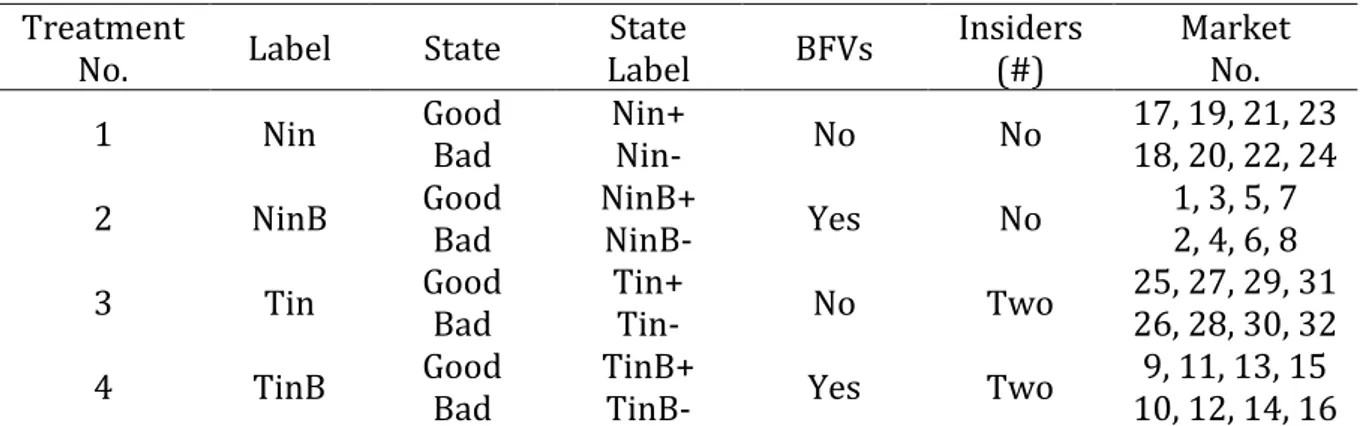
Table 3 displays a summary of the design parameters of each of our 32 asset markets. Specifically, it gives an overview over the underlying state, the provision of BFVs, and the presence of insiders in each market.
9 When markets with or without insider information are considered together, regardless of the provision
12
Table 3: Markets and Information Levels Treatment
No. Label State Label State BFVs Insiders (#) Market No. 1 Nin Good Bad Nin+ Nin- No No 17, 19, 21, 23 18, 20, 22, 24 2 NinB Good Bad NinB+ NinB- Yes No 1, 3, 5, 7 2, 4, 6, 8 3 Tin Good Bad Tin+ Tin- No Two 25, 27, 29, 31 26, 28, 30, 32 4 TinB Good Bad TinB+ TinB- Yes Two 10, 12, 14, 16 9, 11, 13, 15 Note: Markets are numbered in the order how the observations were collected during the experimental
13
3. Informational Models and Hypotheses
3.1. Informational ModelsFollowing the studies of, for example, Plott and Sunder (1982, 1988) or Camerer and Weigelt (1991), we test two different models: the prior information equilibrium (PI) model and the fully revealing rational-expectations equilibrium (RE) model. Both models assume traders to be risk-neutral and give different forecasts about trading behavior of differently informed traders. These models can be formalized quantitatively and tested against each other.10
The PI-model states that traders do not learn from price signals and only use their prior information to determine the state. They ignore the informational content of market prices (as the aggregated information of others) and speculation possibilities depending on the actions of other traders (Palan 2009). Traders only use Bayes' rule to update their expectations about the true state.
The RE-model additionally states that in equilibrium all traders behave as if they are aware of the entire information of all traders in the market. Thus even uninformed traders have the ability to supplement their prior (“private”) information with private information of others via price signals from the market that entail (perfect) information of insiders.11 They are aware of the relationship between the market price, the
underlying state, and their gains from trade and utilize the market price and their “private” information in their demand decision (Tirole 1982).
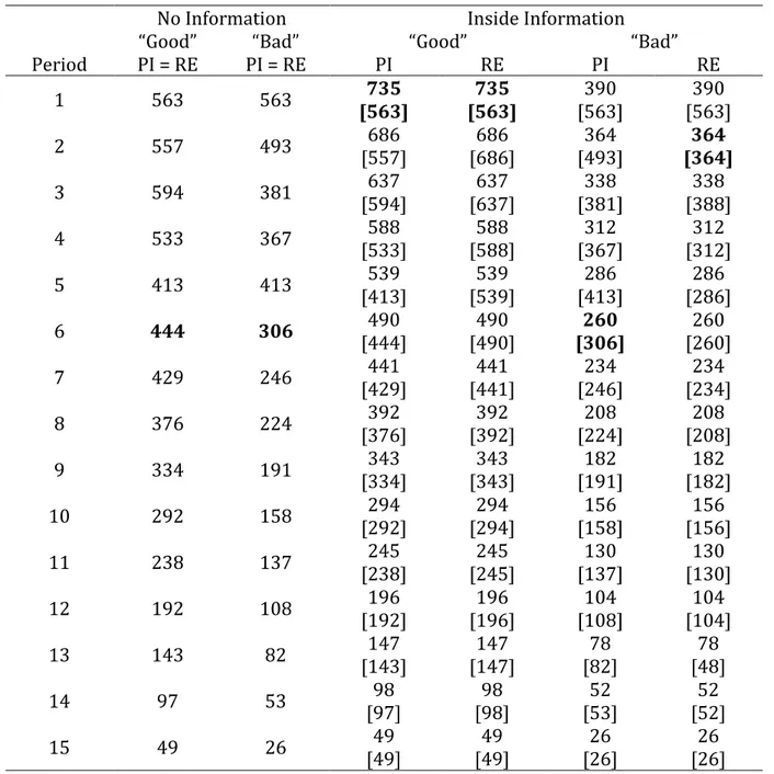
In our experiment we chose dividends, prior probabilities of dividends, and states in a manner that fundamentals and hence predictions of the PI- and RE-models clearly differ in both states. Table 4 shows the expected FVs per asset with respect to information, state, and informational model. When there is no inside information in the market, the PI- and the RE-model both predict no trade in both states. According to both theories, all traders have the same expectations about the respective FVs, which equal the updated BFVs. There are no evident gains from and thus no incentives to trade.
When insider information is present, both theories predict that trade will take place since in- and outsiders have different expectations about fundamentals. For the RE-model this is true only for the first period. Assuming in- and outsiders are strict payoff maximizers and place bid prices marginally below and ask prices marginally above their expected FVs, the market price will approximately average the expected FVs.
10 We refrain from testing intermediate dynamic models like that of Jordan (1982). These models aren't
easy to handle and don't give precise predictions of expected values and therefore prices. Though some works showed that trading in experimental asset markets does seem to follow a kind of “Jordan path” (Plott and Sunder 1982).
11 The RE-model has a close connection to the efficient markets hypothesis. Bid/ask prices reflect diverse
private information and thus induce trading actions identical to those if all traders had all market information (Harrison and Kreps 1978).
14
Table 4: Expected FVs under PI and RE by Information and State
No Information Inside Information
“Good” “Bad” “Good” “Bad”
Period PI = RE PI = RE PI RE PI RE 1 563 563 [563] 735 [563] 735 [563] 390 [563] 390 2 557 493 [557] 686 [686] 686 [493] 364 [364] 364 3 594 381 [594] 637 [637] 637 [381] 338 [388] 338 4 533 367 [533] 588 [588] 588 [367] 312 [312] 312 5 413 413 [413] 539 [539] 539 [413] 286 [286] 286 6 444 306 [444] 490 [490] 490 [306] 260 [260] 260 7 429 246 [429] 441 [441] 441 [246] 234 [234] 234 8 376 224 [376] 392 [392] 392 [224] 208 [208] 208 9 334 191 [334] 343 [343] 343 [191] 182 [182] 182 10 292 158 [292] 294 [294] 294 [158] 156 [156] 156 11 238 137 [238] 245 [245] 245 [137] 130 [130] 130 12 192 108 [192] 196 [196] 196 [108] 104 [104] 104 13 143 82 [143] 147 [147] 147 [82] 78 [48] 78 14 97 53 [97] 98 [98] 98 [53] 52 [52] 52 15 49 26 [49] 49 [49] 49 [26] 26 [26] 26
Notes: Figures show for the case of insider information the known FVs for informed and expected FVs for
[uninformed] traders. The bold figures identify the convergence period as defined in Section 4.1.
Since in the first period the resulting market price is higher (lower) than the BFV of 563 in the “good” (“bad”) state, outsiders supplement their prior information with this price signal and are able to infer the correct state under the RE-model assumptions. Informed traders can thus only take advantage of their superior position in the first period. On the other hand, under the PI-model trade may virtually take place throughout all periods, assuming availability of assets on the supply side. Since market participants ignore the informational content of market prices, expectations about fundamentals only converge slowly to the true value, which leads to a more persistent superior position of insiders. According to both models, bid and ask behavior will result in asset allocations where
15
insiders hold more (less) assets in the “good” (“bad”) state than outsiders. This is especially true under the PI-model.
3.2. Hypotheses
To facilitate the illustration of the results in the following section our analysis focuses around six hypotheses.
Hypothesis 1: Trading prices converge toward the actual FV under all treatment
conditions, but the convergence is faster in markets with insider information and markets where traders are provided with BFVs.
In our markets, convergence toward fundamentals depends substantially on the accuracy of the probability assessment. This is a complex task, especially in an experimental situation, where time is limited. Markets aggregate information. However, it will take time for prices to track the FV.12 Following Romer (1993), the dissemination
of privately held information and/or expectations is likely to cause lagged price movements. Proponents of the “efficiency camp” of insider trading argue that convergence of market prices toward fundamentals is faster when inside information is present (Manne 1984, Engelen and Liedekerke 2007, McGee 2008). Sutter et al. (2012) and Dufwenberg et al. (2005) provide experimental evidence that markets where some traders have an informational/experiential edge above others show a significantly better performance in terms of market efficiency. Since people are unlikely to carry out Bayesian inference by themselves (Kahneman and Tversky 1972, Camerer 1999, Rabin and Schrag 1999), we expect markets where traders are provided with BFVs to converge faster toward fundamentals than markets that are not.
Hypothesis 2: Bubbles occur, but the introduction of asymmetrically informed traders, or
the provision with BFVs significantly reduces the occurrence and extent of bubbles.
A vast literature shows that the bubble-and-crash phenomenon is strikingly robust in SSW markets (see footnote 3). Since the introduction of insider information is expected to enhance market performance in terms of the duration of equilibrium adjustment of market prices, we expect markets with asymmetrically informed traders to be less prone to bubble formation than markets with symmetrically informed traders, a result also observed by Sutter et al. (2012) and Dufwenberg et al. (2005). Similarly, given that markets that are provided with BFVs are expected to converge faster toward fundamentals than markets that are not, we also expect them to exhibit smaller bubbles.
12 Forsythe et al. (1984) argue that “investors bring only their private information to the market and only
after traders have observed prices will they learn the information necessary to achieve the [fully revealing rational-expectations equilibrium].” (p. 973)
16
Hypothesis 3: In early periods, trading behavior of uninformed traders differs from that
of informed traders but converges along with the market price toward that of informed traders. Uninformed traders learn to grasp the correct state and to trade accordingly.
Informed traders condition their trading behavior on private information and uninformed traders adapt their trading behavior based on the belief that informed traders only trade if it is advantageous for them to do so (King 1991), thereby revealing gradually the underlying state. In a fully revealing RE all private information held by informed traders is (sooner or later) revealed via the market price (King 1991). To the same extent as information is revealed, we expect that an adaptation of the trading behavior of in- and outsiders takes place.
Hypothesis 4: In the “good” state, we expect insiders to hold more assets than outsiders,
and in the “bad” state, outsiders to hold more assets than insiders.
Given the different information structures of in- and outsiders, we expect the two types to show a significantly different buying and selling behavior. In Table 4 above we calculate the FV expectations of in- and outsiders. Based on these calculations we derive that insiders buy/hold more assets in the “good” state and outsiders in the “bad” state, under both the PI- and RE-assumption. The predicted asymmetric asset distribution should at least hold true in earlier periods, since we expect outsiders to learn in the course of the market.
Hypothesis 5: Informed traders have a trading advantage and earn superior profits. Given that, especially in the beginning of the markets, insiders are able to buy and sell their assets for advantageous prices they should benefit from their superior informational position.
Hypothesis 6: Elicited price expectations and actual market prices are highly correlated.
Thereby, we expect predictive power to be greater in markets with inside information, and in markets where traders are provided with BFVs.
There is a certain circularity in the market-price development process since current prices depend on expectations about future prices; but both are simultaneously influenced by current price levels and trends (Ball and Charles A. Holt 1998). Self-fulfilling price expectations can render observed market prices independent of the asset's fundamentals, leading to bubbles, in which even rational traders get involved in the expectation of even “greater fools”.13 Expectations should therefore provide crucial
information about the market price development.
13 Such bubbles are referred to as “rational growing bubbles” (Camerer 1989) or simply “rational bubbles”
(Diba and Grossman 1988a, 1988b). They “reflect a self-confirming belief that the stock price depends on a variable (or a combination of variables) that is intrinsically irrelevant” (Diba and Grossman 1988a, p. 520). Porter and Smith (1995) however find that “subjects report a tendency to think that if the market turns [when the bubble bursts] they will be able to sell ahead of the others, but then are “amazed” at the speed with which the crash occurs.” (p. 513)
17
4. Experimental Results
4.1. Equilibrium Adjustment of Prices
Figure 1 illustrates the main findings of our experiment by showing the course of the average equilibrium market prices in our four treatments. Each curve in the four graphs represents four markets under equal conditions with respect to state, insider information, and the provision of BFVs. All four graphs show the tendency of convergence toward the correct state. Most intriguing, the ubiquitous tendency of earlier laboratory asset markets with well-defined declining fundamental value and inexperienced traders to exhibit a well-known bubble-and-crash pattern is not observed in this aggregated examination, independent of the provided information structure. Strikingly, trade in both states starts, regardless of the presence of insiders and/or the provision of BFVs, on aggregate closer to fundamentals in the “bad” state, indicating risk aversion for the average trader.14 Indeed, we find slight risk aversion for the average
trader in our risk pretests and in the personal assessment of one’s own attitude toward risk in the ex-post questionnaire (see Appendix A, Table A. 1 to Table A. 4). Given that average risk attitudes are very similar in all markets, we cannot find a significantly negative Spearman correlation between the average risk-aversion measure in a market and the 1st period market price.15 However, when counting the number of risk-averse
(not risk-neutral, or risk-loving) traders per market, we find a slightly significant Spearman correlation for Risk-Test 1 following Holt and Laury (2002) (𝜌 = -.3049, p-value = .0897, N = 32). Despite the substantial initial deviations from fundamentals (especially in the “good” state), we observe a clear tendency of convergence of aggregate market prices toward fundamentals of the actually underlying state around the fifth period. Intuitively, convergence starts in either state somewhere between the two fundamentals. This implies that we should observe convergence from below in the “good” state and convergence from above in the “bad” state. In the following we explore Hypothesis 1.
While markets on aggregate show a clear convergence pattern, individual markets show substantial diversity. Some markets perform much better than others in terms of convergence toward the FV of the underlying state. Ten out of 32 observed markets even never converge to it.16 We consider market prices as “converged” if they approach the
respective FV as close as ±20% and stay in this range until the end of the market or no more trading takes place. For the very last periods, our definition of convergence
14 Since dividend draws can be considered as lotteries, trading prices below (above) fundamentals
indicate risk aversion (loving) of the average market participant. Hence, the ratio of the realized price and the fundamental value can serve as a proxy for average risk attitude in a market (Chen et al. 2004).
15 The algebraic signs point in the intuitive direction that higher risk aversion in a market leads to a lower
starting price. Only for “Risk-Test 2b” the sign is counterintuitive.
16 Markets 4, 6, 9, 10, 15, 21, 26, 28, 30, 32 never converged toward the FV of the actual underlying state
18
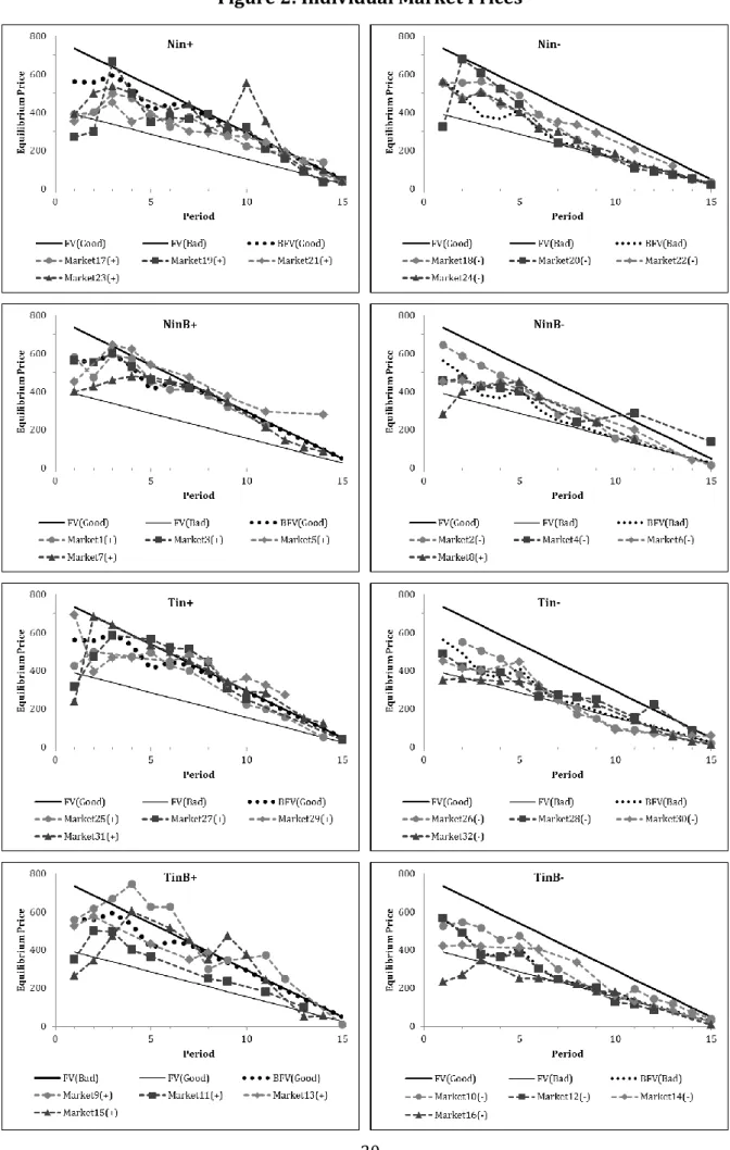
requires at least two consecutive periods without trading, when market prices previously have deviated out of the range.17 Figure 2 shows the course of individual
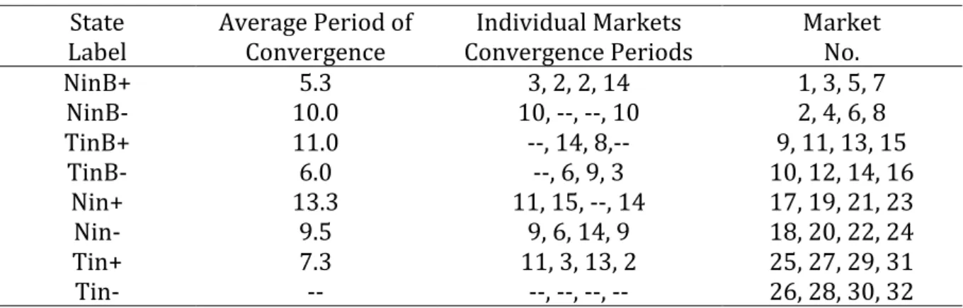
market prices for all markets in the four treatments. As seen, market prices initially fluctuate more erratically, but converge in most cases, sooner or later, toward the genuine state. Table 5 presents the average convergence period by treatment and the individual market convergence periods for the markets that have converged.
To test for general convergence, we count for each treatment the number of markets that have converged. Applying one-sided binomial tests to the number of converged versus the number of non-converged markets, we find a significant tendency of convergence only for Nin, where seven out of eight markets converge (p-value = .0039). The hypothesis of general convergence is neither confirmed for NinB nor for Tin or TinB markets, when analyzed separately.
When pooling the Nin and NinB markets, we observe 13 of 16 markets to converge, which yields statistical significance for general convergence (p-value = .0106, one-sided binomial test). Pooling Tin and TinB markets, we observe only 9 out of 16 markets to converge, implying no statistical significance. This indicates that the presence of insiders does not enhance but rather defer market convergence. On the other hand, confidence intervals for the absolute deviations from fundamentals are for the majority of periods narrower for Tin(B) than for Nin(B) markets. Although not statistically significant, this suggests that the above result lack of convergence in Tin(B) markets is driven by the small number of independent markets.
Result 1: Using our simple counting measure, we only observe a general convergence
toward fundamentals in Nin(B) markets. Our test for general convergence indicates that the presence of insiders defers convergence. This result, however, might be an artifact produced by the relatively small sample size. The provision of 𝐵𝐹𝑉𝑠 has no effect on convergence.
17 This “rule” has been relaxed/adjusted in some markets, where the measure in the last five periods
trespassed the range in only one period, but was adhered to before, so that the assumption of convergence seems prudent. This “correction” has the aim to obtain a more “organic” and adequate measure of convergence. When no trading occurs, no pair of traders is willing to trade away from fundamentals, indicating that all traders are aware of the actual FV and that it is common knowledge (as defined by Aumann 1976). There is no opportunity to “fool” another trader.
19
Figure 1: Average Market Prices
The trajectory of average market prices exhibits clear differences in comparison to most of earlier experiments using the SSW framework. Even in Nin markets the price course resembles that of markets with experienced traders or markets with a composition of traders with mixed information or experience levels (see, for example, Dufwenberg et al. 2005, Haruvy et al. 2007, Hussam et al. 2008, Sutter et al. 2012). Additionally, convergence, as we have defined it, occurs on average later than predicted by the PI- and RE-models,18 except for NinB+ and Tin-. We thus conclude that neither the PI- nor the
RE-model provide indeed good approximations of asset markets in our symmetric and asymmetric information settings. This finding stands in contrast to the previously mentioned literature on markets involving one-period assets and asymmetric information.
18 Both, the PI- and RE-models, predict convergence to occur (as we define it) in the sixth period in both
states, when no insiders are present. The PI-model predicts convergence in the first and in the sixth period and the RE-model predicts convergence in the first and in the second period, in the “good” and “bad” state, respectively, when insiders are present.
20
21
Table 5: Average Convergence Period State
Label Average Period of Convergence Convergence Periods Individual Markets Market No.
NinB+ 5.3 3, 2, 2, 14 1, 3, 5, 7 NinB- 10.0 10, --, --, 10 2, 4, 6, 8 TinB+ 11.0 --, 14, 8,-- 9, 11, 13, 15 TinB- 6.0 --, 6, 9, 3 10, 12, 14, 16 Nin+ 13.3 11, 15, --, 14 17, 19, 21, 23 Nin- 9.5 9, 6, 14, 9 18, 20, 22, 24 Tin+ 7.3 11, 3, 13, 2 25, 27, 29, 31 Tin- -- --, --, --, -- 26, 28, 30, 32
Notes: Markets that did not converge are denoted by “--“. Averages are computed using converged
markets only.
4.2. Over- and Undervaluation of Market Prices
This chapter focuses on Hypothesis 2. As mentioned earlier, bubbles didn’t occur in aggregated form. However, some markets exhibited patterns that, though smaller than in many previous experiments, can be considered as price bubbles. In the following, we define a price bubble as a deviation of market prices from fundamentals by more than 30% in at least two consecutive periods. Since markets firstly must somehow fathom the actually underlying state, we consider, however, only deviations after the fifth period, in the “bad” state. Otherwise, in the “bad” state, market prices in the first periods would often misleadingly signal bubbles, when in fact just the “natural” adaption process takes place. Given our definition of market convergence, a bubble can evidently only occur before a market converges.
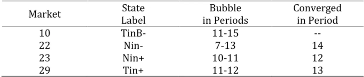
Using our definition of bubbles, we find four markets (10, 22, 23, and 29) to exhibit a bubble pattern. Market 9, the market with the, at the first glimpse, ostensibly most obvious deviation pattern, exceeds fundamentals in the 4th period by “only” 27%, and is
thus not considered to exhibit a bubble pattern. Table 6 gives an overview of markets that exhibit bubble patterns, the duration of the bubble and the convergence period. The occurrence of bubbles seems to have no relation to the presence of insiders, the provision of BFVs, or the underlying state.
To additionally gauge the severity of market-price deviations from fundamentals, i.e., differences in market performance, also when markets don’t exhibit bubble patterns, we employ two deviation measures,19 both developed by Stöckl et al. (2010).
19 Given the high correlation of these deviation measures with other calculated “bubble” measures we
restrain our analysis with the focus on these potentially most reliable measures, RD and RAD. These measures are robust to variations in the number of market periods, the determination of the FV and dividend distribution/variation.
22
Table 6: Markets Exhibiting Bubble Patterns
Market Label State in Periods Bubble Converged in Period
10 TinB- 11-15 --
22 Nin- 7-13 14
23 Nin+ 10-11 12
29 Tin+ 11-12 13
The applied average bias measure for a market calculates the relative deviation (RD) as the average difference between the market price (𝑃𝑡) and the fundamental value (𝐹𝑉𝑡)
normalized by the average fundamental value (𝐹𝑉̅̅̅̅). It measures the average relative distance between the market price and the fundamental value. A value of ±0.1 indicates that the assets are on average overvalued (undervalued) by 10% relative to the average fundamental value. 𝑅𝐷 = 1 15∑ ( 𝑃𝑡− 𝐹𝑉𝑡 𝐹𝑉 ̅̅̅̅ ) 15 𝑡=1 (2)
The applied average dispersion measure for a market calculates the relative absolute deviation (RAD) as the average absolute difference between the market price (𝑃𝑡) and the fundamental value (𝐹𝑉𝑡) normalized by the average fundamental value (𝐹𝑉̅̅̅̅). It
measures the average absolute distance between the period market price and the fundamental value. A value of 0.1 indicates that the assets price differs on average by 10% from the average fundamental value.
𝑅𝐴𝐷 = 1 15∑ ( |𝑃𝑡− 𝐹𝑉𝑡| 𝐹𝑉 ̅̅̅̅ ) 15 𝑡=1 (3)
Both measures are used to get a first impression of differences in price deviations from fundamentals between treatments. We conduct two-sided Mann-Whitney U tests with the null hypothesis of no difference for both deviation measures. Table 7 displays the results. RDs are not significantly different when compared by treatment, due to the fact that negative deviations in the “good” and positive deviations in the “bad” state cancel each other out. The comparison of RADs shows that the provision of BFVs is only conducive to market performance when no insiders are present. The presence of insiders enhances performance compared to the situation without insiders, however, only when no BFVs are given. The performance of markets where insiders are present and BFVs are given together is indistinguishable to markets where only one of these features is at work.
To check the robustness of the results above and for a deeper understanding of potential factors that influence price formation and thus over- or undervaluation of equilibrium markets prices, we conduct panel-regressions with markets as cross sections (𝑚 =
23
1, . . . , 32). The dependent variable is derived from the above mentioned RD measure (Stöckl et al. 2010), denoted in percent. It is defined as:
𝑅𝐷𝑚𝑡 =
𝑃𝑚𝑡− 𝐹𝑉𝑡 𝐹𝑉
̅̅̅̅ , (4)
where 𝑅𝐷𝑚𝑡 measures the difference between the market price of period 𝑡 (𝑃𝑡) and the
respective fundamental value (𝐹𝑉𝑡), normalized by the average fundamental value (𝐹𝑉̅̅̅̅) (Stöckl et al. 2010). The index 𝑚 denotes the market.
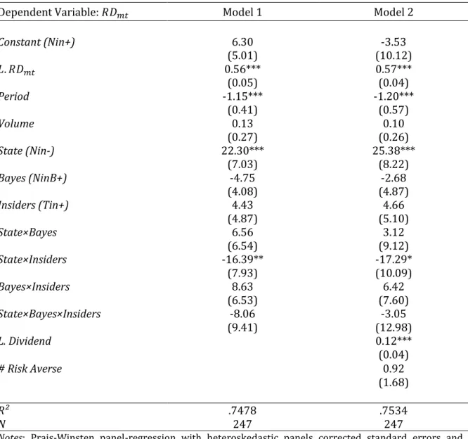
We control for treatment effects by using dummy variables for different treatment features (considering Nin+ as the control group) and their interactions. In particular, we control for the “state of the world” (𝑆𝑡𝑎𝑡𝑒, which is equal to one in the “bad” state and zero otherwise), for the provision of BFVs (𝐵𝑎𝑦𝑒𝑠, which is one when BFVs are given and zero otherwise), and for the presence of insiders (𝐼𝑛𝑠𝑖𝑑𝑒𝑟𝑠, which is equal to one, when insiders are present, and zero otherwise). Additionally, we control for autocorrelation by inclusion of the dependent variable with a lag of one period (L. RD), for a time trend within markets by inclusion of a period variable (𝑃𝑒𝑟𝑖𝑜𝑑), and for the trading volume (𝑉𝑜𝑙𝑢𝑚𝑒). Furthermore we included the drawn dividend in the prior period (𝐿. 𝐷𝑖𝑣𝑖𝑑𝑒𝑛𝑑) and the number of risk-averse traders within a market (# 𝑅𝑖𝑠𝑘 𝐴𝑣𝑒𝑟𝑠𝑒) as explanatory variables. The results are shown in Table 8.
Since both regression models shown in Table 8 display qualitatively the same results, we focus our analysis on Model 2. The model shows that price deviations are strongly path-dependent; a price deviation in the previous round (𝐿. 𝑅𝐷) has a significantly positive effect on the current price deviation. Price deviations decrease over time as participants gain trading experience. 𝑃𝑒𝑟𝑖𝑜𝑑 has a significantly negative effect on price deviation. The last dividend (𝐿. 𝐷𝑖𝑣𝑖𝑑𝑒𝑛𝑑) has a significantly positive (euphoriant price boosting) effect, the higher the dividend in the previous period the larger the price deviation in the current period. Trading activity as measured by 𝑉𝑜𝑙𝑢𝑚𝑒 has no significant effect, just as the number of risk-averse traders within a market (# 𝑅𝑖𝑠𝑘 𝐴𝑣𝑒𝑟𝑠𝑒).
Turning to the effects of treatment features, we see that “bad”-state markets exhibit significantly larger price deviations then “good”-state markets, a non-surprising finding, consistent with the prior nonparametric analysis.
24
Table 7: Relative and Absolute Deviation Measures
Comparison by Nin NinB p-value Tin TinB p-value
Bayesa RD 0.058 0.074 .8336 0.015 0.018 .9164
RAD 0.291 0.195 .0357 0.176 0.200 .5286
Nin Tin p-value NinB TinB p-value
Insidera RD 0.058 0.015 .8336 0.074 0.018 .5286
RAD 0.291 0.176 .0033 0.195 0.200 .7527
Comparison by Nin+ Nin- p-value NinB+ NinB- p-value
Stateb RD -0.202 0.319 .0209 -0.095 0.243 .0209
RAD 0.242 0.339 .0209 0.124 0.265 .0433
Tin+ Tin- p-value TinB+ TinB- p-value
Stateb RD -0.097 0.128 .0209 -0.113 0.148 .0433
RAD 0.149 0.203 .1489 0.185 0.214 .7728
Nin+ NinB+ p-value Nin- NinB- p-value Bayesb RAD RD -0.202 0.242 -0.095 0.124 .0833 .0209 0.319 0.339 0.243 0.265 .2482 .2482
Tin+ TinB+ p-value Tin- TinB- p-value Bayesb RAD RD -0.097 0.149 -0.113 0.185 .7728 .3865 0.128 0.203 0.148 0.214 .5637 .7728
Nin+ Tin+ p-value Nin- Tin- p-value Insiderb RAD RD -0.202 0.242 -0.097 0.149 .0833 .0209 0.319 0.339 0.128 0.203 .0209 .0209
NinB+ TinB+ p-value NinB- TinB- p-value Insiderb RAD RD -0.095 0.124 -0.113 0.185 .7728 .2482 0.243 0.265 0.148 0.214 .3865 .3865 Notes: Mann-Whitney U test, two-sided: a N = 16 (8/8), b N = 8 (4/4).
The provision of BFVs has no effect in both states, when the utilized control variables are considered. This contradicts the nonparametric result. We do not expect that this lack of difference is caused by the fact that traders were actually able to calculate BFVs in the setting where they were not provided. But traders seem to be intuitively able to anticipate approximated BFVs. The presence of insiders is only significant, i.e., exerting a negative (price deviation decreasing) effect in “bad”-state markets,20 a finding that
requires further analysis for a proper understanding.
We are able to calculate the treatment effects (coefficients), given that treatments are comprised of combinations of several features. These coefficients are presented in Table 9 in descending order in terms of the coefficient size. The calculated coefficients are equal to the ones that result out of a regression with treatments as dummy variables and Nin+ as baseline.
20 This outcome is, as explained later, driven by the fact that Nin+ and Tin+ markets are not statistically
25
Table 8: Regressions for RDs of Market Prices from Fundamentals
Dependent Variable: 𝑅𝐷𝑚𝑡 Model 1 Model 2
Constant (Nin+) 6.30 -3.53 (5.01) (10.12) 𝐿. 𝑅𝐷𝑚𝑡 0.56*** 0.57*** (0.05) (0.04) Period -1.15*** -1.20*** (0.41) (0.57) Volume 0.13 0.10 (0.27) (0.26) State (Nin-) 22.30*** 25.38*** (7.03) (8.22) Bayes (NinB+) -4.75 -2.68 (4.08) (4.87) Insiders (Tin+) 4.43 4.66 (4.87) (5.10) State×Bayes 6.56 3.12 (6.54) (9.12) State×Insiders -16.39** -17.29* (7.93) (10.09) Bayes×Insiders 8.63 6.42 (6.53) (7.60) State×Bayes×Insiders -8.06 -3.05 (9.41) (12.98) L. Dividend 0.12*** (0.04) # Risk Averse 0.92 (1.68) R² .7478 .7534 N 247 247
Notes: Prais-Winsten panel-regression with heteroskedastic panels corrected standard errors and
panel-specific autocorrelation (AR1) (Beck and Katz 1995). 32 markets as cross sections with a maximum of 15 observations over time (unbalanced). Only periods where trade took place are considered. Standard errors are shown in parentheses. *, **, and *** indicate significance at the 10%, 5%, and 1% levels, respectively.
Using these coefficients we are able to disentangle differences between treatments by conducting meaningful comparisons which consist of three comparisons for each treatment: (1) a comparison with the counterpart in the “bad”/”good” state, (2) a comparison with the counterpart where BFVs are/are not provided, and (3) a comparison with the counterpart where insiders are/are not present, respectively. We conduct Wald tests to test for the equality of estimated coefficients for these comparisons. The results can be retraced via Table 10, where all possible comparisons are shown and significant differences are highlighted as bold figures.
26
Table 9: Treatment Effects on RDs of Market Prices from Fundamentals in Model 2 Treatment Effect of… Coefficient p-value
NinB- S+B+SB 25.82 .000 Nin- S 25.38 .002 TinB- S+B+I+SB+SI+BI+SBI 16.56 .000 Tin- S+I+SI 12.75 .004 TinB+ B+I+BI 8.40 .062 Tin+ I 4.66 .361 Nin+ --- -3.53 .727 NinB+ B -2.68 .582
Notes: S = State (“Bad”), B = BFVs (provided), I = Insiders (present).
Our finding that “bad” state markets exhibit significantly larger price deviations then “good”-state markets is confirmed with the exception of Tin markets, where deviations in the “bad” state are larger, however, statistically insignificant. The result that the provision of BFVs has no effect is unambiguously confirmed. Moreover, as already seen, the presence of insiders significantly reduces price deviations in “bad”-state markets, leading to an improved market performance.
Furthermore, the presence of insiders leads to an increase of the deviation measure in the “good” state which, given that “good”-state markets tend to trade below fundamentals, leads to an improvement in market performance, i.e., deviations from FVs are smaller in absolute terms, when insiders are present; however, the difference between Nin+ and Tin+ is not significant. Thus, these findings confirm and broaden the prior findings of the nonparametric analysis.
Result 2: Bubbles occur but are infrequent. The nonparametric analysis indicates that the
introduction of insiders reduces bubbles, measured by RD and RAD, however, only when BFVs are not provided. The provision with BFVs significantly reduces deviations, however, only when no insiders are present. The performance of markets where insiders are present and BFVs are given together is not distinguishable from markets where only one of these ingredients is at work. The panel analysis refines and demerges the previous results and indicates that the introduction of insiders improves market performance (measured by