Estimation Risk in Financial Risk Management

Texte intégral

(1)2004s-15. Estimation Risk in Financial Risk Management Peter Christoffersen, Sílvia Gonçalves. Série Scientifique Scientific Series. Montréal Avril 2004. © 2004 Authors. Tous droits réservés. All rights reserved. Reproduction partielle permise avec citation du document source, incluant la notice ©. Short sections may be quoted without explicit permission, if full credit, including © notice, is given to the source..

(2) CIRANO Le CIRANO est un organisme sans but lucratif constitué en vertu de la Loi des compagnies du Québec. Le financement de son infrastructure et de ses activités de recherche provient des cotisations de ses organisations-membres, d’une subvention d’infrastructure du ministère de la Recherche, de la Science et de la Technologie, de même que des subventions et mandats obtenus par ses équipes de recherche. CIRANO is a private non-profit organization incorporated under the Québec Companies Act. Its infrastructure and research activities are funded through fees paid by member organizations, an infrastructure grant from the Ministère de la Recherche, de la Science et de la Technologie, and grants and research mandates obtained by its research teams. Les organisations-partenaires / The Partner Organizations PARTENAIRE MAJEUR . Ministère du développement économique et régional [MDER] PARTENAIRES . Alcan inc. . Axa Canada . Banque du Canada . Banque Laurentienne du Canada . Banque Nationale du Canada . Banque Royale du Canada . Bell Canada . BMO Groupe Financier . Bombardier . Bourse de Montréal . Caisse de dépôt et placement du Québec . Développement des ressources humaines Canada [DRHC] . Fédération des caisses Desjardins du Québec . GazMétro . Hydro-Québec . Industrie Canada . Ministère des Finances [MF] . Pratt & Whitney Canada Inc. . Raymond Chabot Grant Thornton . Ville de Montréal . École Polytechnique de Montréal . HEC Montréal . Université Concordia . Université de Montréal . Université du Québec à Montréal . Université Laval . Université McGill ASSOCIE A : . Institut de Finance Mathématique de Montréal (IFM2) . Laboratoires universitaires Bell Canada . Réseau de calcul et de modélisation mathématique [RCM2] . Réseau de centres d’excellence MITACS (Les mathématiques des technologies de l’information et des systèmes complexes) Les cahiers de la série scientifique (CS) visent à rendre accessibles des résultats de recherche effectuée au CIRANO afin de susciter échanges et commentaires. Ces cahiers sont écrits dans le style des publications scientifiques. Les idées et les opinions émises sont sous l’unique responsabilité des auteurs et ne représentent pas nécessairement les positions du CIRANO ou de ses partenaires. This paper presents research carried out at CIRANO and aims at encouraging discussion and comment. The observations and viewpoints expressed are the sole responsibility of the authors. They do not necessarily represent positions of CIRANO or its partners.. ISSN 1198-8177.

(3) Estimation Risk in Financial Risk Management* Peter Christoffersen†, Sílvia Gonçalves ‡. Résumé / Abstract La valeur-à-risque (VaR) et la mesure ES (Expected Shortfall) sont de plus en plus utilisées pour la mesure du risque d’un portefeuille, l'allocation de capital de risque et la détermination des performances. Les gestionnaires de risques financiers sont donc légitimement intéressés par la précision des techniques classiques de la valeur-à-risque et de la mesure ES. Le but de cet article est précisément d’évaluer la précision des modèles classiques et de mesurer l'importance de l'erreur d'estimation en construisant des intervalles de confiance autour des prévisions de la valeur-à-risque et de la mesure ES. Un des problèmes clés dans la construction d’intervalles de confiance appropriés provient de la dynamique de la variance conditionnelle typiquement observée pour les rendements spéculatifs. Notre article propose donc une technique de ré-échantillonnage qui tient compte de l'erreur d'estimation des paramètres des modèles dynamiques de la variance d’un portefeuille. Une analyse Monte Carlo nous montre que les méthodes généralement utilisées par les praticiens, telles que la simulation historique qui calcule le quantile empirique à l’aide d’une fenêtre mobile des rendements, génèrent des intervalles de confiance pour la valeur-à-risque à 90% qui sont trop étroits et qui contiennent seulement 20% des vraies valeurs-à-risque. D'autres méthodes qui tiennent compte correctement de la dynamique conditionnelle de la variance, telles que la simulation historique filtrée, génèrent quant à elles des intervalles de confiance de la valeur-àrisque à 90% qui contiennent près de 90% des vraies valeurs-à-risque. Les mesures ES sont généralement moins précises que les mesures de valeur-à-risque et les intervalles de confiance autour de la mesure ES sont également moins fiables. Mots clés : gestion des risques, Bootstrap, GARCH. *. We are grateful to Sean Campbell, Valentina Corradi, Frank Diebold, Jin Duan, René Garcia, Éric Jacquier, Simone Manganelli, Stefan Mittnik, Nour Meddahi, Matt Pritsker, Éric Renault, and Enrique Sentana for helpful comments. FCAR, IFM2 and SSHRC provided financial support. The usual disclaimer applies. † Peter Christoffersen is at the Faculty of Management, McGill University, 1001 Sherbrooke Street West, Montreal, Quebec, Canada H3A 1G5, Phone: (514) 398-2969, Fax: (514) 398-3876, Email: peter. christoffersen@mcgill.ca, Web: www.christo.ersen.ca. ‡ Sílvia Gonçalves is at Département de sciences économiques, Université de Montréal, C.P.6128, succ. CentreVille, Montréal, Québec, Canada H3C 3J7, Phone: (514)343-6556, Fax: (514)343-7221, Email: silvia.goncalves@umontreal.ca, Web: http://mapageweb.umontreal.ca/goncals..

(4) Value-at-Risk (VaR) and Expected Shortfall (ES) are increasingly used in portfolio risk measurement, risk capital allocation and performance attribution. Financial risk managers are therefore rightfully concerned with the precision of typical VaR and ES techniques. The purpose of this paper is exactly to assess the precision of common models and to quantify the magnitude of the estimation error by constructing confidence bands around the point VaR and ES forecasts. A key challenge in constructing proper confidence bands arises from the conditional variance dynamics typically found in speculative returns. Our paper suggests a resampling technique which accounts for parameter estimation error in dynamic models of portfolio variance. In a Monte Carlo study we find that commonly used practitioner methods such as Historical Simulation, which calculates the empirical quantile on a moving window of returns, implies 90% VaR confidence intervals that are too narrow and that contain as few as 20% of the true VaRs. Other methods which properly account for conditional variance dynamics, such as Filtered Historical Simulation instead imply 90% VaR confidence intervals that contain close to 90% of the true VaRs. ES measures are generally less accurate than VaR measures and the confidence bands around ES are also less reliable. Keywords: Risk management, boostrapping, GARCH Codes JEL : G12.

(5) 1. Motivation. Value-at-Risk (VaR) and Expected Shortfall (ES) are increasingly used in portfolio risk measurement, risk capital allocation and performance attribution, and financial risk managers are rightfully concerned with the precision of typical VaR and ES techniques. VaR is defined as the conditional quantile of the portfolio loss distribution for a given horizon (typically a day or a week) and for a given coverage rate (typically 1% or 5%), and the ES is defined as the expected loss beyond the VaR. The VaR and ES measures are thus statements about the left tail of the return distribution and in realistic sample sizes (500 or 1000 daily observations) such statements are likely to be made with considerable error. The purpose of this paper is twofold: First, we want to assess the loss of accuracy from estimation error when calculating VaR and ES. Second, we want to assess our ability to quantify ex-ante the magnitude of this error via the construction of confidence bands around the VaR and ES measures. This issue of estimation risk for VaR has been considered previously in the i.i.d. return case by for example Jorion (1995), Pritsker (1997), Chapell and Dowd (1999) and Dowd (2000). But a key challenge in constructing proper VaR and ES confidence bands arises from the conditional variance dynamics typically found in speculative returns. We quantify these dynamics using the celebrated GARCH models of Engle (1982) and Bollerslev (1986). Due to its ability to capture salient features of the return dynamics in very parsimonious and easily estimated specifications, GARCH has become the workhorse model in financial risk management. Nevertheless, and surprisingly, very little is known about the uncertainty in the GARCH VaR and ES forecasts arising from parameter estimation error.1 Our paper extends the resampling technique of Pascual, Romo and Ruiz (2001), which accounts for parameter estimation error in dynamic models of portfolio variance, to the case of VaR and ES forecasts. To our knowledge no asymptotic theory has been established for calculating confidence bands for risk measures in this context. In a Monte Carlo study we find that commonly used practitioner VaR methods such as Historical Simulation, which calculates the empirical quantile on a moving window of returns, imply nominal 90% confidence intervals for the one-day, 1% VaR that are too narrow and that contain as few as 20% of the true VaRs. Other methods which properly account for conditional variance dynamics, such as Filtered Historical Simulation (FHS) suggested by Hull and White (1998) and Barone-Adesi et al (1999), instead imply 90% VaR confidence intervals that contain close to 90% of the true VaRs. Similarly, and importantly, we find that it is in general more difficult to construct accurate confidence bands for the ES measure. All the confidences bands from risk models we consider tend to contain the true ES less frequently than the 90% they should. The 90% confidence bands for ES are thus too narrow in general. The resampling technique we propose can be relatively easily extended to longer horizons, to multivariate risk models, and to allowing for model specification error. In related work Figlewski (2002) computes effective coverages of VaRs with nominal coverages equal to .5, 1 and 5%. He finds that ignoring estimation error causes the effective 1 Baillie and Bollerslev (1992) construct approximate prediction intervals for GARCH variance forecasts at multiple horizons but ignore estimation error. Furthermore, risk management suveys and textbooks such as for example Christoffersen (2003), Dowd (1998) Duffie and Pan (1997), and Jorion (2000) give little or no attention to the estimation error issue.. 2.

(6) coverage to be below the nominal coverage, particularly for the smallest nominal coverage. Whereas Figlewski (2002) focuses on the average coverage of the point forecast VaR allowing for estimation risk, our focus here is to construct confidence bands around the point forecast VaR and ES. Accurate confidence bands reported along with the VaR point estimate will facilitate the use of VaR in active portfolio management as the following example illustrates: Consider a portfolio manager who is allowed to take on portfolios with a VaR of up to 15% of the current capital. If the risk manager calculates the actual point estimate VaR to be 13% with a confidence band of 10-16% then the cautious portfolio manager should rebalance the portfolio to reduce risk. Relying instead only on the point estimate of 13% would not signal any need to rebalance. The remainder of the paper is organized as follows. Section 2 presents our conditionally nonnormal GARCH portfolio return generating process and defines five risk models which we will consider in the subsequent analysis. Section 3 presents the resampling methods used to generate the VaR and ES confidence bands. Section 4 presents the Monte Carlo setup and discusses the results we obtained. Finally, Section 5 concludes and suggests avenues for future research.. 2. Model and Risk Measures. In this paper we model the dynamics of the daily losses (the negative of returns) on a given financial asset or portfolio according to the model Lt = σ t εt , t = 1, . . . , T,. (1). where εt are i.i.d. with mean zero, variance one, and distribution function G. In particular, we focus on the case in which G is a standardized Student’s t distribution with d degrees of freedom,2 i.e. p d/ (d − 2)εt ∼ t (d) . To model the volatility dynamics we use a symmetric GARCH(1,1) model for σ2t : σ 2t = ω + αL2t−1 + βσ 2t−1 , where α + β < 1. The GARCH(1,1) model with standardized Student’s t distribution has been very successful in capturing the volatility clustering and nonnormality found in daily asset return data. See for example Bollerslev (1987) and Baillie and Bollerslev (1989). Although we focus on this particular model of returns, our approach applies to more complex models of σ 2t and/or to other distributions for εt . At a given point in time, we are interested in describing the risk in the tails of the conditional distribution of losses over a given horizon, say one-day, using all the information available at that time. We consider two popular risk measures. One is the Value-at-Risk (VaR), which is simply a conditional quantile of the losses distribution. The other is the Expected Shortfall (ES), which measures the expected losses over the next day given that losses exceeds VaR. 2. The model can be generalized to allow for skewness following Theodossiou (1998).. 3.

(7) The VaR measure for time T + 1 with coverage probability p, based on information at time T , is defined as the (positive) value V aRTp +1 such that ¡ ¢ Pr LT +1 > V aRTp +1 |F T = p, (2). where F T denotes the information available at time T . Typically p is a small number, e.g. p = 0.01 or p = 0.05. Similarly, we define the ES measure for time T + 1 with coverage probability p, given information at time T , as the (positive) value ESTp +1 such that ¡ ¢ ESTp +1 = E LT +1 |LT +1 > V aRTp +1 , F T . (3) Given model (1), we can obtain simplified expressions for V aRTp +1 and ESTp +1 . More specifically, we can show that V aRTp +1 = σ T +1 G−1 1−p ≡ σ T +1 c1,p ,. (4). where G−1 1−p denotes the (1 − p)-th quantile of G, the distribution of standardized losses εt = Lt /σ t , and σ T +1 is the conditional volatility for time T + 1. For instance, if G is the −1 standard normal distribution Φ and p = 0.05, we have that G−1 1−p = Φ0.95 = 1.645, and thus p V aRT +1 = 1.645σ T +1 . In the general case where ε ∼ G, equation (4) shows that we can express V aRTp +1 as the product of σ T +1 with a constant c1,p ≡ G−1 1−p , whose value depends on G and on p. Similarly, under model (1), we can show that ¡ ¢ ESTp +1 = σ T +1 E ε|ε > G−1 (5) 1−p ≡ σ T +1 c2,p ,. where ε is an i.i.d. random variable with mean zero, variance one, and distribution G. If φ(a) ε ∼ N (0, 1), we can show that E (ε|ε > a) = 1−Φ(a) , for any constant a, where φ and Φ denote the density and the distribution functions of a standard normal random variable. φ(Φ−1 ) Thus, in this particular case, ESTp +1 = σ T +1 p1−p . When the innovation distribution is not the standard normal, this formula does not ¡ ¢ apply. However, we can still express the ES as σT +1 times a constant c2,p ≡ E ε|ε > G−1 1−p whose value is a function of G and p. In our simulations below, where G is a standardized Student’s t (d) distribution, we computed c2,p by Monte Carlo simulation using 100, 000 simulations from the appropriate distribution G. In practice, we cannot compute the true values of V aRTp +1 and ESTp +1 , since they depend on the characteristics of the data generating process (i.e. they depend on G and on the conditional variance model σ 2T +1 ). Thus, we need to estimate these measures, which introduces estimation risk. Our ultimate goal in this paper is to quantify the estimation risk by constructing a confidence — or prediction — interval for the true but unknown risk measures. We will consider six different estimation methods, divided into three groups.. 2.1. Historical Simulation. The first and most commonly used method is referred to as Historical Simulation (HS). It calculates VaR and ES using the empirical distribution of past losses. In particular, the HS estimate of V aRTp +1 is given by HS-V aRTp +1 = Q1−p ({Lt }) , 4.

(8) where Q1−p ({Lt }) denotes the (1 − p)-th empirical quantile of the losses data {Lt }Tt=1 . The HS estimate of ESTp +1 is given by   X 1 ¢ Lt  , HS-ESTp +1 = ¡ # Lt > HS-V aRTp +1 p Lt >HS-V aRT +1. ¢ ¡ where # Lt > HS-V aRTp +1 denotes the number of observations of {Lt }Tt=1 that are above the HS estimate of VaR. The HS method is completely nonparametric and does not depend on any distributional assumption, thus capturing the nonnormality in the data. It nevertheless ignores the potentially useful information in the volatility dynamics.. The estimation methods that we consider next take into account the volatility dynamics by explicitly relying on the GARCH(1,1) model for predicting σ T +1 . In particular, given (4) and (5), estimates of V aRTp +1 and ESTp +1 can be obtained in three steps: 1. Estimate the GARCH(1,1) parameters through Gaussian QMLE, maximizing 1 X ¡ 2¢ ln L ∝ − ln σ t + 2 t=1 T. µ. Lt σt. ¶2. .. ³ ´ Given the QML estimates ω ˆ, α ˆ , βˆ , we can compute the variance sequence σ ˆ 2t and σ t from the past observed squared losses and the past the implied residuals ˆεt = Lt /ˆ estimated variance using the recursion ˆ σ2, ˆ +α ˆ L2t + βˆ σ ˆ 2t+1 = ω t where σ ˆ 21 = 1−ˆαωˆ−βˆ , the unconditional variance of Lt . A prediction of σ T +1 is given by σ ˆ T +1 , where σ ˆ 2T +1 = ω ˆ +α ˆ L2T + βˆ σ ˆ 2T . 2. Choose values for the constants c1,p and c2,p . Call these cˆ1,p and cˆ2,p , respectively. 3. Compute the estimates of V aRTp +1 and ESTp +1 as p Vd aRT +1 = σ ˆ T +1 cˆ1,p p c T +1 = σ ES ˆ T +1 cˆ2,p .. We can distinguish between two groups of methods according to rule used to choose the constants c1,p and c2,p in step 2: fully parametric methods and nonparametric methods.. 5.

(9) 2.2. Parametric Methods. These methods postulate a distribution G and use it to compute cˆ1,p and cˆ2,p . We consider two leading cases: one based on the (erroneous) assumption of conditional normality and another based on the (true) assumption of Student’s t (d) distribution. Normal Conditional Distribution Erroneously imposing the normal distribution on the innovation term εt gives the following estimates of V aRTp +1 and ESTp +1 : N-V aRTp +1 = σ ˆ T +1 cˆN 1,p N-ESTp +1 = σ ˆ T +1 cˆN 2,p , where −1 cˆN 1,p = Φ1−p , ¢ ¡ φ Φ−1 1−p N , cˆ2,p = p. with Φ−1 1−p the (1 − p)-th quantile of a standard normal distribution. We will call this the “Normal” method. Student Conditional Distribution Instead, imposing the true Student’s t distribution implies the following estimates of the risk measures: t-V aRTp +1 = σ ˆ T +1 cˆt1,p t-ESTp +1 = σ ˆ T +1 cˆt2,p , where p (d − 2) /dt−1 d,1−p ³ ´ p = E ε|ε > (d − 2) /dt−1 1−p ,. cˆt1,p = cˆt2,p. with t−1 d,1−p the (1 − p)-th quantile of the Student’s t distribution with d degrees of freedom t and cˆ2,p the truncated expectation of ε, a random variable following a standardized t (d) distribution. We compute the truncated expectation by simulation, as explained above. This will be called the “Student” method. Given the distributional assumption on G, no estimation is involved in computing c1,p and c2,p . Thus, obtaining a prediction interval for the risk measures is equivalent to obtaining a prediction interval for σ ˆ T +1 . The main disadvantage of these methods is the parametric assumption on the standardized losses. The “Normal” method imposes conditional normality, which does not hold for real data. Instead, the “Student” method imposes the (true) conditional Student’s t (d) distribution and is therefore unrealistic. Even if standardized losses follow a Student t distribution, in practice the number of degrees of freedom d needs to be estimated, thus introducing some estimation error which is not taken into account by this method. We consider both methods for comparison purposes. 6.

(10) 2.3. Nonparametric Methods. These methods estimate c1,p and c2,p using the implied GARCH(1,1) residuals ˆεt = Lt /ˆ σt. They differ in the way they use the residuals to compute cˆ1,p and cˆ2,p . Extreme Value Theory The Extreme Value Theory (EVT) approach estimates c1,p and c2,p under the assumption that the tail of the conditional distribution of the GARCH innovation is well approximated by an heavy-tailed distribution. This approach was proposed by McNeil and Frey (2000), who derived estimates of c1,p and c2,p based on the maximum likelihood estimator of the parameters of a Generalized Pareto Distribution (GPD). Here, we suppose that the tail of the conditional distribution of εt is well approximated by the distribution function F (z) = 1 − L (z) z −1/ξ ≈ 1 − cz −1/ξ , whenever εt > u, where L (z) is a slowly varying function that we approximate with a constant c, and ξ is a positive parameter. u is a threshold value such that all observations above u will be used in the estimation of ξ. We let Tu denote the number of observations that exceed u. The Hill estimator (Hill, 1975) ˆξ corresponds to the MLE estimator of ξ under the assumption that the standardized residuals ˆεt are approximately i.i.d. It is defined as Tu X ¡ ¢ ˆξ = 1 ln ˆε(T −t+1) − ln (u) , Tu t=1 where ˆε(t) denote the t-th order statistic of ˆεt (i.e ˆε(t) ≥ ˆε(t−1) for t = 2, . . . , T ). The important choice of Tu will be discussed at the beginning of the Monte Carlo Results section below. ˆ Given ˆξ, an estimate of the tail distribution F is obtained by choosing c = TTu u1/ξ , which derives from imposing the condition 1 − F (u) = TTu . We thus obtain the following estimate of F : Tu ³ z ´−1/ˆξ . Fˆ (z) = 1 − T u The EVT approach relies on Fˆ (z) to estimate the constants c1,p and c2,p . In particular, the −1 , the (1 − p)th-quantile of the tail distribution Fˆ . We can estimate of c1,p is equal to Fˆ1−p show that ¶−ˆξ µ T Hill cˆ1,p = u p . Tu ´ ³ −1 ˆ ˆ Similarly, to compute an estimate of c2,p we use F (z) to compute E ε|ε > F1−p , where ε ∼ i.i.d. Fˆ . We can show that the following closed form expression holds true −1 ´ ³ Fˆ1−p −1 . = E ε|ε > Fˆ1−p 1 − ˆξ. 7.

(11) This implies the following Hill’s estimate of c2,p : cˆHill 2,p =. cˆHill 1,p . 1 − ˆξ. The Hill’s estimates of V aRTp +1 and ESTp +1 are given by Hill-V aRTp +1 = σ ˆ T +1 cˆHill 1,p Hill-ESTp +1 = σ ˆ T +1 cˆHill 2,p , respectively. Gram-Charlier and Cornish-Fisher Expansions This method relies on the Cornish-Fisher and Gram-Charlier expansions to approximate the conditional density of the standardized losses εt . For a standardized random variable, a Gram-Charlier expansion produces an approximate density function that can be viewed as an expansion of the standard normal density augmented with terms that capture the effects of skewness and excess kurtosis. Thus, Gram-Charlier expansions are a convenient tool to account for departures of conditional normality.3 The Cornish-Fisher expansion approximates the inverse cumulative density function directly. The approximation to c1,p is thus: −1 CF1−p. =. Φ−1 1−p. where. i γ2 h ¡ i i γ h¡ ¢ ¢ γ 1 h¡ −1 ¢2 2 1 −1 3 −1 −1 3 −1 Φ1−p − 1 + Φ1−p − 3Φ1−p − 2 Φ1−p − 5Φ1−p , + 6 24 36 ¡ ¢ γ 1 = E ε3 ¡ ¢ γ 2 = E ε4 − 3,. with ε ∼ G (0, 1). We will refer to the expansions methods generically as GC (for GramCharlier). Thus, we have d −1 cˆGC 1,p = CF 1−p , −1. −1 d 1−p is the sample analogue of CF1−p , i.e. it replaces γ 1 and γ 2 with their sample where CF σt: analogues evaluated on the standardized residuals ˆεt = Lt /ˆ. γˆ 1 γˆ 2. T 1X 3 = ˆε T t=1 t. T 1X 4 = ˆε − 3. T t=1 t. Thus, we obtain the following estimate of V aRTp +1 :. ˆ T +1 cˆGC GC-V aRTp +1 = σ 1,p . 3. For an application of Gram-Charlier expansions in finance, see Backus, Foresi, Li and Wu (1997) and references therein.. 8.

(12) Similarly, we can define an approximation to c2,p that relies on the Gram-Charlier and Cornish-Fisher expansions. In particular, we can show that ¢ ¡ −1 ³ h¡ i γ i´ ¡ ¢ φ CF1−p ¢ ¢ γ 1 h¡ 2 GC −1 −1 2 −1 −1 2 c2,p = E ε|ε > CF1−p = CF −3 . 1+ CF1−p − 1 + CF1−p 1−p p 6 24 The Gram-Charlier estimate of ESTp +1 is given by. ˆ T +1 cˆGC GC-ESTp +1 = σ 2,p , −1 GC where cˆGC 2,p is obtained from c2,p by replacing CF1−p , γ 1 and γ 2 with their sample analogues. When G is the standard normal distribution, the Gram-Charlier estimates of VaR and ES coincide with those obtained with the “Normal” method.. Filtered Historical Simulation The Filtered Historical Simulation (FHS) method estimates c1,p and c2,p from the empirical distribution of the (centered) residuals. Thus it combines a model-based variance with a data-based conditional quantile. Several papers including Hull and White (1998), Barone-Adesi et al (1999), and Pritsker (2001) have found the FHS method to perform well. The FHS estimates of c1,p and c2,p are given by ³© ªT ´ cˆF1,pHS = Q1−p ˆεt − ˆε t=1. and. cˆF2,pHS.  X ¢ ¡ 1 ¢ = ¡ ˆεt − ˆε  , # ˆεt − ˆε > cˆF1,pHS ˆ ε >ˆ cF HS . t. PT −1. 1,p. where ˆε = T εt . Centered residuals are considered because their sample average is t=1 ˆ zero by construction, thus better mimicking the true mean zeroPexpectation of the standardized errors εt . If a constant is included in the losses model, Tt=1 ˆεt = 0 and centering of the residuals becomes irrelevant. This implies the following FHS estimates of V aRTp +1 and ESTp +1 : F HS-V aRTp +1|T = σ ˆ T +1 cˆF1,pHS ES-V aRTp +1 = σ ˆ T +1 cˆF2,pHS .. 3. Resampling Methods for Estimation Risk. In this section we describe the bootstrap methods we use to assess the estimation risk in the risk estimates presented above. Our first bootstrap method applies to Historical Simulation. This bootstrap method ignores any volatility dynamics and simply treats losses as being i.i.d. This “naive” bootstrap method generates pseudo losses by resampling with replacement from the set of original losses, according to the following algorithm: 9.

(13) Bootstrap Algorithm for Historical Simulation Risk Measures Step 1. Generate a sample of T bootstrapped losses {L∗t : t = 1, . . . , T } by resampling with replacement from the original data set {Lt }. Step 2. Compute the HS estimates of VaR and ES on the bootstrap sample: ³ ´ ∗p ∗ T HS-V aRT +1 = Qp {Lt }t=1 . HS-EST∗p+1 =. . 1 ¡ ∗ ¢ # Lt > HS-V aRT∗p+1. X. ∗p L∗t >HS-V aRT +1. . L∗t  .. Step 3. Repeat Steps 1 and 2 a large number of times, B say, and o obtain a sequence of n ∗p(i) bootstrap HS risk measures. For instance, HS-V aRT +1 : i = 1, . . . , B denotes a sequence of bootstrap VaR measures. We set B = 999 in our Monte Carlo simulations below. Step 4. The 100 (1 − α) % bootstrap prediction interval for V aRTp +1 is given by µn µn · oB ¶ oB ¶¸ ∗p(i) ∗p(i) HS-V aRT +1 HS-V aRT +1 , Q1−α/2 , Qα/2 i=1. i=1. o n ∗p(i) where Qα (·) is the α−quantile of the empirical distribution of HS-V aRT +1 . A similar bootstrap interval can be computed for ESTp +1 . Following the Historical Simulation approach, this naive bootstrap method is completely nonparametric, avoiding any distributional assumptions on the data. However, by implicitly assuming that returns are i.i.d., this method fails to capture the dependence in returns when it exists. In particular, as our simulations will show, this method of computing confidence bands for risk measures is not appropriate when returns follow a GARCH model. The validity of the bootstrap for financial data depends crucially on its ability to correctly mimic the dependence properties of returns. A natural and often used bootstrap method for GARCH models consists of resampling with replacement the standardized residuals, the idea being that the standardized errors are i.i.d. in the population. The bootstrap returns are then recursively generated using the GARCH volatility dynamic equation and the resampled standardized residuals. The bootstrap methods that we describe next are based on this general idea. As described in the previous section, under model (1), the VaR and ES have the following simplified expressions V aRTp +1 = σ T +1 c1,p ,. (6). ESTp +1 = σ T +1 c2,p,. (7). and where c1,p and c2,p are a function of G and p, and σT +1 is given by the square root of σ 2T +1 = ω + αL2T + βσ 2T . 10. (8).

(14) Given (6) and (7), there are two sources4 of risk associated with predicting V aRTp +1 and using information available at T . One is the uncertainty in computing c1,p and c2,p . If the risk model correctly specifies G, then this source of risk is not present. The other source of risk relates to predicting the volatility σ T +1 using day T ’s information. For our GARCH(1,1) model, it is easy to see that σ 2T +1 depends on information available at day T and on the unknown parameters ω, α and β. In particular, using the GARCH equation (8), we can write σ 2T as a function of past losses as follows: ESTp +1. σ 2T. µ ¶ ∞ X ω ω j 2 +α . = β LT −j−1 − 1−α−β 1−α−β j=0. Replacing ω, α and β with their MLE estimates yields σ ˆ 2T. =. ω ˆ 1−α ˆ − βˆ. +α ˆ. T −2 X j=0. µ βˆ L2T −j−1 −. ω ˆ. j. 1−α ˆ − βˆ. ¶. ,. (9). ˆ σ 2 . The need to estimate the GARCH which delivers a point estimate σ ˆ 2T +1 = ω ˆ +α ˆ L2T + βˆ T parameters introduces the second source of estimation risk. The presence of estimation risk in computing V aRTp +1 and ESTp +1 is our main motivation for using the bootstrap to obtain prediction intervals for these risk measures. The bootstrap methods we use are based on Pascual, Romo and Ruiz (2001), who proposed a bootstrap method for building prediction intervals for returns volatility σ t based on the GARCH(1,1) model. In particular, for the nonparametric methods, we extend the Pascual, Romo and Ruiz (2001) resampling scheme to the case of V aRTp +1 and ESTp +1 by using the bootstrap to account for estimation error not only in σT +1 but also in the constants c1,p and c2,p that multiply σ T +1 . Bootstrap Algorithm for GARCH-Based Measures of Risk Step 1. Estimate the GARCH model by MLE and compute the centered residuals ˆεt −ˆε, ˆ T denote the empirical distribution function of ˆεt . where ˆεt = Lσˆ tt , t = 1, . . . , T. Let G Step 2. Generate a bootstrap pseudo series of portfolio losses {L∗t : t = 1, . . . , T } using the recursions ˆ ˆ ∗2 , = ω ˆ +α ˆ L∗2 σ ˆ ∗2 t−1 + β σ t t−1 ˆ ∗t ε∗t , for t = 1, . . . , T L∗t = σ ˆ T and where σ ˆ ∗2 ˆ 21 = 1−ˆαωˆ−βˆ . With the bootstrap pseudo-data {L∗t }, where ε∗t ∼ i.i.d.G 1 = σ ∗ compute the bootstrap MLE’s ω ˆ ∗, α ˆ ∗ and βˆ . Step 3. Obtain a bootstrap prediction of volatility σ ˆ ∗T +1 according to ˆ ∗ ˆ ∗2 , ˆ∗ + α ˆ ∗ L∗2 σ ˆ ∗2 T +β σ T +1 = ω T In general, model risk is a third source of uncertainty when forecasting V aRTp +1 and ESTp +1 . Here, we abstract from this source of uncertainty since we take the GARCH model of returns as being correctly specified. 4. 11.

(15) given the initial values L∗T = LT , = σ ˆ ∗2 T. ω ˆ∗ ∗ 1−α ˆ − βˆ ∗. +α ˆ∗. T −2 X. βˆ. j=0. ∗j. Ã. L2T −j−1 −. ω ˆ∗ ∗ 1−α ˆ ∗ − βˆ. !. .. (10). Step 4. Compute cˆ∗1,p and cˆ∗2,p , the bootstrap estimates of c1,p and c2,p . These bootstrap estimates are computed exactly in the same fashion as cˆ1,p and cˆ2,p with the difference that they are evaluated on the bootstrap data instead of the real data. In particular, for the parametric methods (Normal and Student), we simply set cˆ∗1,p = cî1,p and cˆ∗2,p = cî2,p for i = N or t, where cî1,p and cî2,p are as described before. In contrast, for the nonparametric methods, we first compute the bootstrap residuals ˆε∗t =. L∗t , σ ˆ ∗t. ∗ ∗2 ∗2 with σ ˆ ∗2 ˆ∗ + α ˆ ∗ Rt−1 + βˆ σ ˆ t−1 and σ ˆ ∗2 ˆ 21 . Next, we evaluate the estimates of c1,p and t = ω 1 = σ c2,p on the data set {ˆε∗t }Tt=1 . For instance, µn oT ¶ ∗ ∗ ∗F HS ˆεt − ˆε . cˆ1,p = Q1−p t=1. Step 5. For each estimation method, compute the bootstrap estimates of V aRTp +1 and using σ ˆ ∗T +1 and cˆ∗1,p and cˆ∗2,p . Step 6. Identical to steps 3 and 4 in the naive bootstrap.. ESTp +1. ˆ, α ˆ Step 3 accounts for the estimation risk in computing σ ˆ T +1 by replacing the estimates ω ∗ ∗ ∗ ∗ ˆ ˆ and β by their bootstrap analogues ω ˆ ,α ˆ and β when computing σ ˆ T +1 . In particular, (10) 2 replicates the way in which σ ˆ T is computed in (9). Notice however that σ ˆ ∗2 T is conditional on the observed past observations on the losses {Lt : t = 1, . . . , T } , not on the bootstrap losses generated in step 2, implying that it is small when the (true) losses are small at the end of the sample and large when they are large. Depending on the estimation method, step 4 computes a bootstrap estimate of the risk measure that may or may not take into account the estimation risk in computing the constants c1,p and c2,p . In particular, contrary to the nonparametric methods, the Normal and Student methods do not account for this estimation risk as they make a parametric assumption on G. For the FHS method, bootstrap residuals are centered before computing the empirical quantile as a way to enforce the mean zero property on the estimated bootstrap residuals (centering of the residuals is not needed if a constant is included in the returns model since in that case the residuals have mean zero by construction). We conclude this section by noting that it may be possible to apply asymptotic approximations such as the delta-method to calculate prediction intervals for the GARCH variance 12.

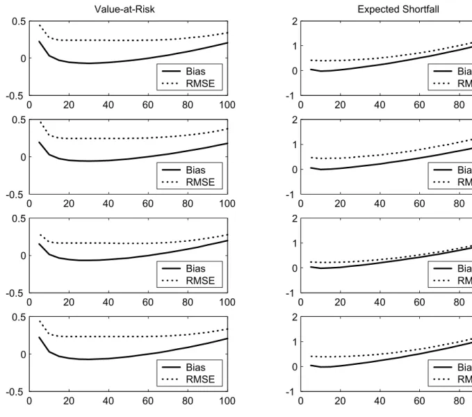
(16) forecast.5 However, it is not at all obvious how to calculate prediction intervals for VaR and ES using the delta method in the nonparametric risk models we consider. Furthermore, even in parametric cases, the approximate delta-method is likely to perform worse than the resampling techniques considered here. In the following we therefore restrict attention to prediction intervals calculated via our resampling technique.. 4. Monte Carlo Results. As indicated in the introduction the purpose of our paper is twofold: First, we want to assess the loss of accuracy from estimation error when calculating VaR and ES. Second, we want to assess our ability to quantify ex-ante the magnitude of this error via the construction of confidence bands around the risk measures. This section provides quantitative evidence on these two issues through a Monte Carlo study. We will consider four versions of the GARCH-t(d) data generating process (DGP) below. In each version we set α = .10 and ω = (202 /252)∗(1 − α − β) . The unconditional volatility is thus 20% per year. Our four chosen parameterizations are: 1) Benchmark: β = .80, d = 8 2) High Persistence: β = .89, d = 8 3) Low Persistence: β = .40, d = 8 4) Normal Distribution: β = .80, d = 500 Recall that before applying the Hill estimator for the extreme value distribution we need to choose a cut-off point, Tu , which defines the sub-sample of extremes from which the tail index parameter will be estimated. In order to pick this important parameter we perform an initial Monte Carlo experiment in which we simulate data from the four DGPs above, estimate the tail index on a grid of cut-off values, and finally compute the resulting bias and root mean squared error measures (RMSEs) from the one-day VaR and ES forecasts. Figures 1 and 2 show the results for the case of 500 and 1,000 total estimation sample points respectively. In each case, we choose a grid of truncation points which correspond to including the 0.5% to 10% largest losses in the sub-sample of extremes. The horizontal axis in each figure denotes the number of included extreme observations (out of 500 and 1,000 respectively), and the vertical axis shows the bias and RMSEs. From the viewpoint of minimizing RMSE subject to achieving a bias that is close to zero, and looking broadly across the four DGPs, it appears that a percentage cut-off of 3% is reasonable for VaR and 1% is reasonable for ES. Notice that we do not want to choose the truncation point on a case by case basis as that would potentially bias the overall results in favor of the Hill-based risk model. In any case the results are quite similar across DGPs and sample sizes but notably different across VaR and ES models, which in itself is an important and useful finding. Tables 1-4 contain the Monte Carlo results corresponding to the four DGPs above. The top half of each table contains the VaR results and the bottom half the ES results. The left half of each table contains the accuracy properties of the point estimates of the relevant risk measure and the right half contains the 90% bootstrap interval properties. For both the VaR and ES forecasts we consider two estimation sample sizes, T = {500, 1000} . 5. This approach is taken for example in Duan (1994).. 13.

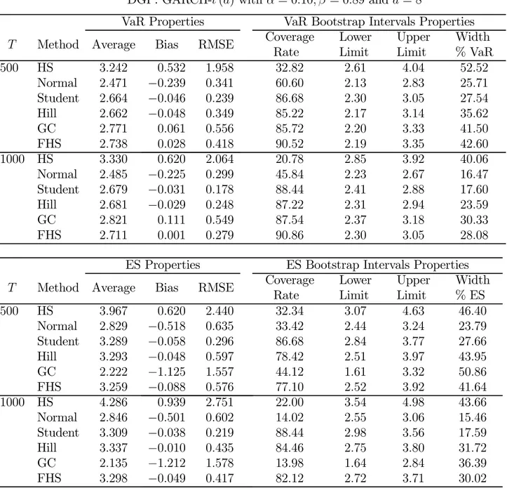
(17) In all the experiments we calculate the properties of the point estimates from 100,000 Monte Carlo replications. For the properties of the bootstrap prediction intervals, we consider only 5,000 Monte Carlo replications, each with 999 bootstrap replications. Any Monte Carlo study of the bootstrap is computationally demanding and this is particularly so in our study due to the nonlinear optimization involved in estimating GARCH.. 4.1. Point Predictions of VaR and ES. While the main focus of our paper is on constructing finite sample prediction intervals of the VaR and ES measures, we first consider the various models’ ability to accurately point forecast the risk measures. The point prediction results on VaR and ES are reported in terms of bias and root mean squared error, which are reported in the left half of each table. 4.1.1. The Benchmark Case. The top panel of Table 1 contains the VaR results for our benchmark DGP when the sample size is T = 500. Considering first the bias of the VaR estimates, the main thing to note is the upward bias of the HS and the downward bias of the Normal. The latter is of course to be expected as the Normal imposes a distribution tail which is too thin for the 1% coverage rate. The other models appear to show only minor biases with the FHS model displaying the smallest bias overall. In terms of the root mean squared error (RMSE) of the VaR estimates, we see that the HS has by far the highest RMSE, followed by the GC model. The Hill model in particular, but also the FHS model, are quite close to the benchmark Student model, which assumes a known degree of freedom equal to 8 and is therefore not a feasible alternative. The RMSE of the Normal is also low but, as mentioned before, displays considerable bias. Increasing the sample size to 1,000 in the second panel of Table 1 implies smaller biases in general. The HS is still biased upwards and the Normal downwards. In terms of RMSE, the Hill and FHS methods perform very well compared with the hypothetical benchmark Student. We next examine the quality of the point predictions of ES by the various models. We now find a very large downward bias for the GC and again for the Normal model. In comparison with the VaR results, the various estimated ES models have RMSEs which are considerably larger than the hypothetical Student model. The increase in RMSE is due partly to increases in the bias. The results for the GC model indicate that it is not useful for ES calculations the way we have implemented it here. Notice that in the ES case the GC model is an aggregate of two approximations: First, the Cornish-Fisher approximation to the VaR and second the Gram-Charlier approximation to the cumulative density. Unfortunately, the two approximation errors appear to compound each other for the purpose of ES calculation. 4.1.2. The High Persistence Case. The top half of Table 2 reports the VaR findings for a DGP of high volatility persistence and therefore also high kurtosis. We see that the biases and RMSEs are comparable to the benchmark DGP in Table 1 for the conditional models but not for the HS model. The HS 14.

(18) model is now even more biased and has a RMSE of more than 50% of the average true VaR, which is approximately 2.71. The Hill and FHS models again perform very well. The bottom half of Table 2 reports results for ES using the high volatility persistence DGP. We find that the results are very close to the bottom half of Table 1 for the conditional models but not for HS. This finding matches the results for VaR reported in the top halves of Tables 1 and 2 respectively. As before, the bias and RMSEs of the HS model are very large, and for the ES the GC model again performs poorly. 4.1.3. The Low Persistence Case. In the top half of Table 3 we consider the VaR case of low volatility persistence which makes the returns close to independent over time. Not surprisingly the HS model performs much better now. Interestingly, the Hill and FHS models perform very well here also. The bottom half of the table shows the results for ES forecasting in the low persistence process. As in the VaR case, we see that the HS model now performs relatively well. 4.1.4. The Conditional Normal Case. The top half of Table 4 contains VaR results for the conditionally normal GARCH DGP. Comparing with Table 1 we see that the bias and RMSEs are considerably smaller now. It is still the case that the HS model is much worse than the conditional models. The Normal model of course performs very well now as it is the true model. Interestingly, the Hill and FHS models which do not directly nest the Normal model still perform decently. This is important as the risk manager of course never knows exactly the degree of conditional non-normality in the return distribution. The bottom half of Table 4 considers the ES risk measure. Comparing the bottom of Table 4 with the bottom of Table 1 we see that the biases and RMSEs are generally much smaller under conditional normality. The biases and RMSEs for ES are very much in line with the ones from VaR in the top half of Table 4. This is sensible from the perspective that under conditional normality the ES does not contribute information over and beyond the VaR.. 4.2. Bootstrap Prediction Intervals for VaR and ES. The above discussion was concerned with the precision of the VaR and ES point forecasts. We now turn our attention to the results for the bootstrap prediction intervals from the different VaR and ES models. That is, we want to assess the ability of the bootstrap to reliably predict ex ante the accuracy of each method in predicting the 1-day-ahead 1% VaR and ES. The prediction interval results are reported in the right hand side of each table. We show the true coverage rate of nominal 90% intervals as well as the average limits of the confidence bands and the average width of the confidence band as a percentage of the true VaR point forecast.. 15.

(19) 4.2.1. The Benchmark Case. Turning back to Table 1 and looking at the top panel, we remark that the historical simulation VaR (HS) bands (calculated from the i.i.d. bootstrap) have a terribly low effective coverage for a promised nominal coverage of 90%. Furthermore, the confidence bands are on average very wide. The HS method ignores the dynamics in the DGP which is costly both in terms of coverage and width.6 The VaR imposing the conditional normal distribution (Normal) has a coverage which is as bad as the HS model but which has a much smaller average width. The small width does of course not offer much comfort here as the nominal coverage is much too small. The benchmark Student model suffers from slight under-coverage but is very narrow. Notice thus that the Student model is not perfect in finite samples. This is because the bootstrap is not able to perfectly capture the GARCH estimation parameter uncertainty for this sample size. Not surprisingly though the Student model with known degree of freedom performs very well overall. The Hill model has lower coverage than the Student and has wider intervals. The GC models has even lower coverage than the Hill and has wider intervals. Finally, the FHS model has slight over-coverage, which is arguably to be preferred to under-coverage, but it also has a fairly wide average coverage interval. In the second panel of Table 1 we increase the risk manager’s sample size to 1,000 past return observations in each simulation. Comparing with the top panel in Table 1 the result are as follows: The HS model coverage actually gets worse with sample size. In the short (500 observations) sample the HS model is able to pick up some of the dynamics in the return process, but it is less able to do so as the sample size increases. The average width is smaller as the sample size increases due to the higher precision in estimating the (unconditional) VaR. The Normal model also has worse coverage and better width. This may seem puzzling, but note that there is no reason to believe that a larger sample size will improve the coverage of a misspecified model. The Student model has around the same coverage and better width compared with the 500 observation case. The estimation error in the GARCH parameters is less of an issue now, which brings the Student model closer to the truth. The Hill and GC models both have better coverages and widths now. Finally, notice that the FHS model also benefits from the larger estimation samples and show better coverages and lower widths. The bottom half of Table 1 reports results for the bootstrap prediction intervals from the different ES models. We notice the following: The Historical Simulation ES bands (calculated from the i.i.d. bootstrap) have a low effective coverage for a promised nominal coverage of 90%. Furthermore the confidence bands on average are quite wide. The HS results for ES are roughly comparable with those for VaR in Table 1. The ES imposing the conditional normal distribution (Normal) has a surprisingly low coverage. Thus, while the normal distribution is bad for VaR prediction intervals it is much worse for ES prediction intervals. The Student model suffers from slight under-coverage but is very narrow. The Hill model has the best coverage of the feasible models but is quite wide. The GC model has very low coverage and quite wide intervals. Finally, the FHS model has considerable 6. We also calculated GARCH-bootstrap confidence intervals for the HS model. These performed better than the iid bootstrap intervals reported in the tables but they were still very inaccurate and were therefore not included in the tables. The iid boostrap is shown here because it is arguably most in line with the model-free spirit of the HS model.. 16.

(20) under-coverage. This is in contrast with the VaR intervals in the top half of the table. Looking more broadly at the results in Table 1, we see that the infeasible Student has the best coverage followed by the Hill and then the FHS model. The HS, Normal and GC models have poor coverage. Compared with the top half of the table it thus appears that while the FHS performs well for VaR prediction interval calculation, it is less useful for ES prediction intervals. The Hill estimator appears to be preferable here. Generally the coverage rates are considerably worse for ES than for VaR. 4.2.2. The High Persistence Case. The top right hand side of Table 2 reports VaR interval results from a return generating process with relatively high persistence. Comparing panel for panel with the benchmark process in Table 1, we notice that the HS model has worse coverage and worse width, whereas the Normal model has better coverage. The Student model has slightly worse coverage. The GC model has similar coverage but wider intervals. The FHS has roughly the same coverage under high persistence but the widths are wider here as well. Thus, the higher persistence associated with higher kurtosis leads to wider prediction intervals overall. The bottom right hand side of Table 2 reports ES results. Comparing the VaR and ES results in Table 2 we see that the coverage rates are typically much worse for ES than VaR. A comparison of the results for ES against the benchmark process in Table 1 reveals that the HS model has worse coverage and worse width. The Normal model has very poor coverage still. The Student model has slightly worse coverage and the width is worse. The Hill model generally has better coverage but wider intervals. The GC model still has very poor coverage. Finally, the FHS has roughly the same coverage under high persistence but the widths are worse here as well. The higher persistence again leads to wider prediction intervals overall. 4.2.3. The Low Persistence Case. The top right hand side of Table 3 reports VaR results from returns with low variance persistence. Not surprisingly the results are reversed from Table 2, which contained high persistence variances. We now find that the HS model has much better coverage and slightly better widths. The low persistence process is closer to i.i.d., the only assumption under which the HS model is truly justified. The Normal model has worse coverages but it has better widths. The Student model has near perfect coverage and better widths. The Hill and GC models have similar coverages and better widths than before. Finally, the FHS model has worse coverages, but the widths are slightly better. The bottom right hand side of Table 3 reports ES results from returns with low variance persistence. We now find that the HS performs much better as we are closer to the i.i.d. case but otherwise the results are similar to the benchmarks in Table 1. 4.2.4. The Conditional Normal Case. In Table 4 we generate returns which are close to conditionally normally distributed. Comparing the VaR panels in Table 4 with the corresponding panels in Table 1, where the. 17.

(21) conditional returns were t(8), we see the following: The HS model now has worse coverage but also lower width than before. The Normal model has better coverage and better width. This is not surprising as the Normal model is now closer to the truth. The Student model has better coverage and better width, probably because the return data generating process is to some degree easier to capture. The Hill and GC models have similar coverage and better width than before. The FHS model also has roughly the same coverage under conditional normality but better width than under the conditional t(8). Not surprisingly, the models generally perform better under conditional normality. It is perhaps surprising that the Hill model performs well under conditional normality as the tail index parameter may be biased in this case. In the bottom half of Table 4 we report the ES results. As expected, the models generally perform better under conditional normality in terms of coverage. The HS model is again notably worse than the other models, the FHS is also worse than the others. The Normal model and the GC model which nests the normal models naturally have very good coverages.. 4.3. Summary of Results. Based on the results in Tables 1-4, we reach the conclusion that the HS model not only gives bad point estimates of VaR and ES estimates (see also Pritsker 2001) but it also implies very poor confidence bands. This is true even when the degree of volatility persistence is relatively modest. The Normal model of course works reasonably well when the normality assumption is close to true in the data but otherwise not. The Hill and FHS models perform quite well, even for the conditionally normal distribution. We noticed also that the GC model has serious problems when calculating ES point estimates and intervals for conditionally non-normal returns. Finally, the FHS model works particularly well for VaR calculations. In general we found that the RMSEs of the feasible models were much higher in percent of the benchmark Student model when calculating ES compared to VaR measures. Thus, while the ES measure in theory conveys more information about the loss distribution tail, it is also harder to estimate precisely. This point is important to consider when arguing over the relative merits of the two risk measures. Unfortunately, it is also much harder to reliably assess ex ante the accuracy of ES measures compared with the VaR measures. While the Hill, GC and particularly the FHS model give quite reliable coverage rates for the 90% confidence bands around the VaR point forecast, the corresponding coverage rates for the ES measure are typically much lower than 90% and thus unreliable. We suspect that the higher bias of the ES forecasts is the culprit of the under-coverage in this case. Notice that from a conservative risk management perspective over-coverage would be preferred to under-coverage. Finally, while the FHS model appears to be preferable for calculating VaR forecasts and forecasts intervals, the Hill model performs well in the ES case. The distribution-free FHS model is useful for quantile forecasting but when the mean beyond the quantile must be forecast, then the functional form estimation implicit in the Hill method adds value.. 18.

(22) 5. Summary and Directions for Future Work. Risk managers and portfolio managers often haggle over the precision of a VaR estimate. A trader faced with a point estimate VaR which exceeds the agreed upon VaR limit may be forced to rebalance the portfolio at an inopportune time. Quantifying the uncertainty of the VaR point estimate is important because it allows for risk managers to make more informed decisions when dictating a portfolio rebalance. Consequently we suggest a bootstrap method for calculating confidence bands around the VaR point estimate. The procedure is valid even under conditional heteroskedasticity and nonnormality, which are important features of speculative asset returns. We find that the FHS VaR models yield confidence bands which have correct coverage but which are also quite wide. VaR models based on parametric assumptions are much narrower but also often too narrow causing under-coverage of the intervals. We also find that the accuracy of ES forecasts is typically much lower than that of VaR forecasts. Furthermore the accuracy of the ES forecasts is harder to quantify ex ante. These findings have important implications for the choice of risk model and risk measure. The directions for future work are several. • So far we have studied the effects of estimation risk at the portfolio level only (See Benson and Zangari, 1997, Engle and Manganelli, 2000, and Zangari, 1997). Many banks rely instead on multivariate risk factor models such as those considered in Glasserman, Heidelberger, and Shahabuddin (2000 and 2002). The issue of estimation risk is probably even more important in the multivariate case. • We only consider one-day ahead VaR and ES in this paper. Extending the horizon of interest would be useful. The interesting thing about the 1-step ahead is that here ONLY estimation risk matters (given the true model). • We want to extend the bootstrap methods described here to account for model risk. • Risk models based on realized volatility models rather than GARCH models may allow for the calculation of VaR and ES prediction intervals from asymptotic theory (See Andersen, Bollerslev, Diebold and Labys, 2003). We plan to explore these types of models in future work. We round off by noting that one of the industry benchmarks, namely RiskMetrics, relies on calibrated rather than estimated parameters and does not allow for the calculation of estimation risk. The issue of VaR uncertainty is nevertheless crucial in those models as well but it is not easily quantified.. 19.

(23) Figure 1: RMSE and Bias of Hill Estimator for Various Truncation Points The Total Sample Consists of 500 Daily Loss Observations. Benchmark. Value-at-Risk 2. 0.5. 1. 0 -0.5. Hi Persist. Expected Shortfall. 1. 0. Bias RMSE 0. 10. 20. 30. 40. 50. 1. 2. 0.5. 1. 0 -0.5. 0. 10. 20. 30. 40. Normal. 0. 10. 20. 30. 0. Bias RMSE 50. 0.5. -1. 40. 50. Bias RMSE 0. 10. 20. 30. 40. 50. 2 1. 0 0. Bias RMSE -0.5. Lo Persist. -1. Bias RMSE. 0. 10. 20. 30. 40. 50. -1. 1. 2. 0.5. 1. 0 -0.5. 10. 20. 30. 40. 0. 10. 20. 30. 0. Bias RMSE 0. Bias RMSE. 50. 20. -1. 40. 50. Bias RMSE 0. 10. 20. 30. 40. 50.

(24) Figure 2: RMSE and Bias of Hill Estimator for Various Truncation Points The Total Sample Consists of 1,000 Daily Loss Observations. Value-at-Risk. Expected Shortfall. Benchmark. 0.5. 2 1. 0 0. Bias RMSE -0.5. 0. 20. 40. 60. 80. 100. Hi Persist. 0.5. 20. 40. 60. 80. 100. 1 0. Bias RMSE 0. 20. 40. 60. 80. 100. 0.5 Normal. 0. 2. 0. -0.5. -1. Bias RMSE 0. 20. 40. 60. 80. 100. 2 1. 0 0. Bias RMSE -0.5. 0. 20. 40. 60. 80. 100. 0.5 Lo Persist. -1. Bias RMSE. -1. Bias RMSE 0. 20. 40. 60. 80. 100. 2 1. 0 0. Bias RMSE -0.5. 0. 20. 40. 60. 80. 100. 21. -1. Bias RMSE 0. 20. 40. 60. 80. 100.

(25) Table 1. 90% Prediction Intervals for 1% VaR and ES: Benchmark Case DGP: GARCH-t (d) with α = 0.10, β = 0.80 and d = 8 VaR Properties T. Method Average. HS Normal Student Hill GC FHS 1000 HS Normal Student Hill GC FHS 500. 3.282 2.866 3.090 3.053 3.194 3.138 3.239 2.872 3.097 3.071 3.245 3.106. Bias. RMSE. 0.176 −0.240 −0.016 −0.053 0.088 0.032 0.133 −0.234 −0.009 −0.035 0.139 0.000. 0.747 0.331 0.243 0.327 0.493 0.383 0.671 0.289 0.179 0.237 0.435 0.268. ES Properties T. Method Average. HS Normal Student Hill GC FHS 1000 HS Normal Student Hill GC FHS 500. 3.966 3.283 3.816 3.765 2.609 3.718 4.020 3.289 3.824 3.815 2.490 3.771. Bias. RMSE. 0.131 −0.552 −0.019 −0.071 −1.226 −0.107 0.185 −0.546 −0.011 −0.020 −1.345 −0.064. 0.978 0.617 0.299 0.544 1.421 0.535 0.894 0.586 0.221 0.397 1.469 0.391. 22. VaR Bootstrap Intervals Properties Coverage Lower Upper Width Rate Limit Limit % VaR 60.44 2.73 4.03 41.80 59.66 2.53 3.19 21.20 88.78 2.73 3.44 22.83 86.04 2.56 3.53 31.19 85.10 2.60 3.67 34.41 90.72 2.57 3.77 38.59 47.52 2.85 3.69 27.11 41.74 2.63 3.09 14.85 88.60 2.83 3.33 16.14 86.80 2.71 3.40 22.27 87.08 2.77 3.63 27.75 90.48 2.70 3.52 26.46 ES Bootstrap Intervals Properties Coverage Lower Upper Width Rate Limit Limit % ES 60.54 3.15 4.61 38.06 20.70 2.90 3.64 19.29 88.78 3.37 4.24 22.68 77.12 2.97 4.45 47.56 42.08 1.98 3.79 47.18 75.42 2.95 4.36 36.75 52.24 3.40 4.57 30.58 7.32 3.01 3.54 13.85 88.60 3.50 4.11 15.94 83.16 3.22 4.36 29.95 13.52 1.98 3.32 35.02 80.52 3.18 4.27 28.49.

(26) Table 2. 90% Prediction Intervals 1% VaR and ES: High Persistence DGP: GARCH-t (d) with α = 0.10, β = 0.89 and d = 8 VaR Properties T. Method Average. HS Normal Student Hill GC FHS 1000 HS Normal Student Hill GC FHS 500. 3.242 2.471 2.664 2.662 2.771 2.738 3.330 2.485 2.679 2.681 2.821 2.711. Bias. RMSE. 0.532 −0.239 −0.046 −0.048 0.061 0.028 0.620 −0.225 −0.031 −0.029 0.111 0.001. 1.958 0.341 0.239 0.349 0.556 0.418 2.064 0.299 0.178 0.248 0.549 0.279. ES Properties T. Method Average. HS Normal Student Hill GC FHS 1000 HS Normal Student Hill GC FHS 500. 3.967 2.829 3.289 3.293 2.222 3.259 4.286 2.846 3.309 3.337 2.135 3.298. Bias. RMSE. 0.620 −0.518 −0.058 −0.048 −1.125 −0.088 0.939 −0.501 −0.038 −0.010 −1.212 −0.049. 2.440 0.635 0.296 0.597 1.557 0.576 2.751 0.602 0.219 0.435 1.578 0.417. 23. VaR Bootstrap Intervals Properties Coverage Lower Upper Width Rate Limit Limit % VaR 32.82 2.61 4.04 52.52 60.60 2.13 2.83 25.71 86.68 2.30 3.05 27.54 85.22 2.17 3.14 35.62 85.72 2.20 3.33 41.50 90.52 2.19 3.35 42.60 20.78 2.85 3.92 40.06 45.84 2.23 2.67 16.47 88.44 2.41 2.88 17.60 87.22 2.31 2.94 23.59 87.54 2.37 3.18 30.33 90.86 2.30 3.05 28.08 ES Bootstrap Intervals Properties Coverage Lower Upper Width Rate Limit Limit % ES 32.34 3.07 4.63 46.40 33.42 2.44 3.24 23.79 86.68 2.84 3.77 27.66 78.42 2.51 3.97 43.95 44.12 1.61 3.32 50.86 77.10 2.52 3.92 41.64 22.00 3.54 4.98 43.66 14.02 2.55 3.06 15.46 88.44 2.98 3.56 17.59 84.46 2.75 3.80 31.72 13.98 1.64 2.84 36.39 82.12 2.72 3.71 30.02.

(27) Table 3. 90% Prediction Intervals 1% VaR and ES: Low Persistence DGP: GARCH-t (d) with α = 0.10, β = 0.4 and d = 8 VaR Properties T. Method Average. HS Normal Student Hill GC FHS 1000 HS Normal Student Hill GC FHS 500. 3.226 2.910 3.137 3.093 3.245 3.179 3.186 2.914 3.142 3.112 3.291 3.147. Bias. RMSE. 0.079 −0.237 −0.010 −0.054 0.098 0.032 0.039 −0.233 −0.005 −0.035 0.144 0.000. 0.464 0.321 0.232 0.318 0.497 0.374 0.382 0.284 0.173 0.233 0.437 0.263. ES Properties T. Method Average. HS Normal Student Hill GC FHS 1000 HS Normal Student Hill GC FHS 500. 3.867 3.333 3.875 3.816 2.648 3.778 3.901 3.337 3.879 3.865 2.528 3.820. Bias. RMSE. −0.019 −0.553 −0.011 −0.072 −1.238 −0.108 0.015 −0.549 −0.007 −0.021 −1.358 −0.066. 0.636 0.608 0.286 0.537 1.412 0.529 0.524 0.581 0.214 0.392 1.458 0.386. 24. VaR Bootstrap Intervals Properties Coverage Lower Upper Width Rate Limit Limit % VaR 82.36 2.72 3.94 38.79 52.02 2.63 3.20 18.12 90.60 2.84 3.45 19.40 85.96 2.64 3.56 29.25 85.06 2.69 3.72 32.75 91.48 2.65 3.81 36.88 75.10 2.83 3.60 24.47 36.22 2.70 3.13 13.66 90.10 2.91 3.38 14.93 87.50 2.77 3.46 21.93 86.98 2.84 3.70 27.33 90.46 2.76 3.58 26.06 ES Bootstrap Intervals Properties Coverage Lower Upper Width Rate Limit Limit % ES 73.52 3.11 4.51 36.05 14.58 3.01 3.67 17.00 90.60 3.50 4.26 19.57 76.04 3.06 4.52 37.66 41.18 2.01 3.84 47.12 73.92 3.03 4.41 35.54 76.18 3.33 4.42 28.04 6.20 3.09 3.59 12.86 90.10 3.60 4.17 14.66 82.88 3.29 4.44 29.55 12.82 2.01 3.36 34.73 80.36 3.25 4.34 28.04.

(28) Table 4. 90% Prediction Intervals 1% VaR and ES: Normal Distribution DGP: GARCH-t (d) with α = 0.10, β = 0.80 and d = 500 VaR Properties T. Method Average. HS Normal Student Hill GC FHS 1000 HS Normal Student Hill GC FHS 500. 3.023 2.889 2.893 2.850 2.874 2.903 2.999 2.895 2.898 2.869 2.889 2.888. Bias. RMSE. 0.122 −0.012 −0.008 −0.051 −0.027 0.002 0.098 −0.006 −0.003 −0.032 −0.012 −0.013. 0.545 0.172 0.172 0.227 0.209 0.255 0.502 0.123 0.123 0.163 0.149 0.179. ES Properties T. Method Average. HS Normal Student Hill GC FHS 1000 HS Normal Student Hill GC FHS 500. 3.447 3.309 3.309 3.271 3.416 3.347 3.480 3.315 3.316 3.304 3.365 3.274. Bias. RMSE. 0.127 −0.011 −0.011 −0.048 0.096 −0.073 0.160 −0.005 −0.004 −0.017 0.045 −0.046. 0.647 0.196 0.196 0.306 0.489 0.308 0.608 0.141 0.141 0.219 0.339 0.221. 25. VaR Bootstrap Intervals Properties Coverage Lower Upper Width Rate Limit Limit % VaR 55.14 2.63 3.50 30.08 88.90 2.61 3.13 17.98 88.90 2.61 3.13 17.98 86.06 2.48 3.17 23.86 86.94 2.53 3.16 21.78 90.88 2.49 3.30 28.01 39.96 2.72 3.30 19.98 89.54 2.70 3.07 12.75 89.76 2.71 3.08 12.75 87.46 2.61 3.10 16.88 87.92 2.65 3.11 15.85 90.36 2.60 3.17 19.64 ES Bootstrap Intervals Properties Coverage Lower Upper Width Rate Limit Limit % ES 54.44 2.92 3.83 27.5 88.86 2.99 3.58 17.83 88.90 2.99 3.58 17.83 80.98 2.78 3.66 26.50 88.10 2.78 4.30 45.93 79.70 2.75 3.62 26.29 41.98 3.09 3.80 21.37 89.68 3.10 3.52 12.64 89.76 3.10 3.52 12.64 85.54 2.95 3.61 19.82 89.90 2.91 3.97 31.91 83.46 2.92 3.57 19.57.

(29) References [1] Andersen, T., Bollerslev, T., Diebold, F.X. and P. Labys (2003), Modeling and Forecasting Realized Volatility, Econometrica , 71, 529-626. [2] Backus, D., S. Foresi, K. Li and L. Wu (1997), Accounting for Biases in Black-Scholes, manuscript, The Stern School at NYU. [3] Baillie, R. and T. Bollerslev (1989), The Message in Daily Exchange Rates: A Conditional Variance Tale, Journal of Business and Economic Statistics, 7, 297-309. [4] Baillie, R. and T. Bollerslev (1992), Prediction in Dynamic Models with Time Dependent Conditional Variances, Journal of Econometrics, 52, 91-113. [5] Barone-Adesi, G., K. Giannopoulos and L. Vosper (1999), VaR without Correlations for Nonlinear Portfolios, Journal of Futures Markets, 19, 583-602. [6] Benson, P. and P. Zangari (1997), A General Approach to Calculating VaR without Volatilities and Correlations, RiskMetrics Monitor, JP Morgan-Reuthers, Second Quarter, 19-23. [7] Bollerslev, T. (1986), Generalized Autoregressive Conditional Heteroskedasticity, Journal of Econometrics, 31, 307-327. [8] Bollerslev, T. (1987), A Conditionally Heteroskedastic Time Series Model for Speculative Prices and Rates of Return,” Review of Economics and Statistics, 69, 542-547. [9] Chapell, D. and K. Dowd (1999), Confidence Intervals for VaR, Financial Engineering News, March. [10] Christoffersen, P. (2003), Elements of Financial Risk Management. San Diego: Academic Press. [11] Dowd. K. (1998), Beyond Value at Risk: The New Science of Risk Management. Chichester and New York: Wiley and Sons. [12] Dowd, K. (2000), Assessing VaR Accuracy, Derivatives Quarterly, 6, 61-63. [13] Duan, J-C. (1994), Maximum Likelihood Estimation Using Price Data of the Derivative Contract, Mathematical Finance, 4, 155-167. [14] Duffie, D. and J. Pan (1997), An Overview of Value at Risk, Journal of Derivatives, 4, 7-49. [15] Engle, R. (1982), Autoregressive Conditional Heteroskedasticity with Estimates of the Variance of United Kingdom Inflation, Econometrica, 50, 987-1007. [16] Engle, R. and S. Manganelli (2000), CAViaR: Conditional Autoregressive Value at Risk by Regression Quantiles, manuscript, NYU Stern and ECB.. 26.

(30) [17] Figlewski, S. (2002), Estimation Error in the Assessment of Financial Risk Exposure, manuscript, the Stern School of Business at New York University. [18] Glasserman, P., P. Heidelberger, and P. Shahabuddin (2000), Variance Reduction Techniques for Estimating Value-at-risk, Management Science, 46, 1349-1364. [19] Glasserman, P., P. Heidelberger, and P. Shahabuddin (2002), Portfolio Value-at-Risk with Heavy-Tailed Risk Factors, Mathematical Finance, 12, 239-270. [20] Hill, B. (1975), A Simple General Approach to Inference about the Tail of a Distribution. Annals of Statistics, 3, 1163—1174. [21] Hull, J. and A. White (1998), Incorporating volatility updating into the historical simulation method for VAR,” Journal of Risk, 1, Fall. [22] Jorion, P. (1996), Risk2 : Measuring the Risk in Value-At-Risk, Financial Analysts Journal, 52, 47-56. [23] Jorion, P. (2000), Value at Risk: The New Benchmark for Managing Financial Risk. Second Edition. New York: MacGraw-Hill. [24] McNeil, A. and R. Frey (2000), Estimation of Tail-Related Risk Measures for Heteroskedastic Financial Time Series: An Extreme Value Approach, Journal of Empirical Finance, 7, 271-300. [25] Pascual, L., J. Romo, and E. Ruiz (2001), Forecasting Returns and Volatilities in GARCH Processes Using the Bootstrap, manuscript, Departamento de Estadistica y Econometria, Universidad Carlos III de Madrid. [26] Pritsker, M. (1997), Towards Assessing the Magnitude of Value-at-Risk Errors Due to Erros in the Correlation Matrix, Financial Engineering News, October/November. [27] Pritsker, M. (2001), The Hidden Dangers of Historical Simulation, Working Paper 2001-27, Federal Reserve Board, Washington, DC. [28] Theodossiou, P. (1998), Financial Data and the Skewed Generalized t Distribution, Management Science, 44, 1650-1661. [29] Zangari, P. (1997), Streamlining the Market Risk Measurement Process, RiskMetrics Monitor, JP Morgan-Reuthers, First Quarter, 29-36.. 27.

(31)