Sensor Validation for On-line Vibration Monitoring
for Second European Workshop on Structural Health Monitoring
Authors:
Gaetan Kerschen Pascal De Boe
Jean-Claude Golinval Keith Worden
1
ABSTRACT
For a reliable on-line vibration monitoring of structures, it is necessary to have accurate sensor information. However, sensors may sometimes be faulty or may even become unavailable due to failure or maintenance activities. The problem of sensor validation is therefore a critical part for structural identifi-cation. The objective of the present study is to present a procedure based on principal component analysis, which is able to perform detection, isolation and reconstruction of a faulty sensor. Its efficiency is assessed using an experimental application.
INTRODUCTION
For a reliable on-line vibration monitoring of structures, it is necessary to have accurate sensor information. However, sensors may sometimes be faulty (e.g. gain fault or damaged sensor) or may even become unavailable due to failure or maintenance activities. The problem of sensor validation is therefore a critical part of structural health monitoring. In this study, sensor validation refers to the capability to detect, isolate and reconstruct a faulty sensor. The present paper aims at presenting a procedure based upon principal component analysis which is able to tackle all these objectives. The proposed methodology is data-driven, i.e., it does not require a structural model, which is an important feature for practical applications. It only assumes that the number of sensors is large enough in order to guarantee redundancy in the measured data set.
1Gaetan Kerschen, Pascal De Boe, Jean-Claude Golinval, Department of Materials, Mechanical and Aerospace Engineering, University of Li`ege, Chemin des Chevreuils 1 (B52), B-4000 Li`ege, Belgium;
Keith Worden, Dynamics Research Group, Department of Mechanical Engineer-ing, University of Sheffield, Sheffield S1 3JD, United Kingdom
PRINCIPAL COMPONENT ANALYSIS
Principal component analysis (PCA) is a multivariate analysis technique which was first introduced by Pearson in 1901 and developed independently by Hotelling in 1933. It is also closely related to proper orthogonal decomposition, also known as Karhunen-Lo`eve transform.
Given an observed nS-dimensional response vector x, the goal of PCA is to
reduce the dimensionality of x. This is realised by finding r principal axes pi
with i = 1, ..., r onto which the retained variance under projection is maximal. These axes, denoted as principal directions or PCA modes, are given by the eigenvectors associated with the r largest eigenvalues of the covariance matrix:
Σ= E[(x − µ)(x − µ)T] (1)
where E[·] is the expectation and µ = E[x] is the mean of the data.
If the principal directions are collected in a matrix P = [p1 ... pr], then
z= PT(x − µ) is a reduced r-dimensional representation of the observed vector
x. Among all linear techniques, PCA provides the optimal reconstruction ˆx = µ+ Pz of xi in terms of the quadratic reconstruction error kx − ˆxk2.
It is worth pointing out that PCA is also closely related to singular value decomposition. If the mean is subtracted from the data and if m observations are collected in a matrix X (nS rows and m columns), then the left singular
vectors of X, as eigenvectors of XXT, are the principal directions. The singular values indicate how the corresponding left singular vectors participate and the right singular vectors are the time coefficient vectors of the principal directions.
SENSOR FAULT DETECTION AND ISOLATION
The purpose of this section is to investigate the problem of sensor fault detec-tion and isoladetec-tion in structural dynamics. Friswell and Inman [1] proposed two approaches based on the comparison between the subspace of the response and the subspace generated by the lower modes of a structural model. In reference [2], the detection of sensor failures lies on an auto-associative neural network which is known to implement PCA. The inputs and the targets of the neural network are merely the measured signals and the network is trained using data which is known to be healthy. During the detection stage, the residual vector between the inputs and the outputs of the network is computed. If the residual of a sensor exceeds a certain threshold whilst the residuals of the other sensors remain relatively low then that sensor is declared as faulty.
In this paper, an approach similar to that adopted in reference [3] for dam-age detection using piezo-sensor array is considered. From the mode accelera-tion method, the system response x(t) to external loading f (t) with a limited frequency bandwidth (ω ωk+1. . .) can be expressed through mode
superposi-tion: x(t) = k X i=1 φiφTi ωiµi Z t 0 f(τ ) sin(ωi(t − τ )) dτ + n X i=k+1 φiφTi ω2 i µi f(t)
=
k
X
i=1
φiαi(t) + r αres(t) (2)
This shows that the system response contains the contribution of the modes which respond dynamically and the contribution of the residual modes which respond statically. Equation (2) suggests that the subspace spanned by the system response does not depend on the excitation signal f (t), provided that the modes in the frequency bandwidth participate to the system response. It should be noted that the system is also assumed to be linear and time invariant. Our interest in PCA lies in the fact that it offers a means of computing the subspace spanned by the data without the need to compute the mode shapes. Indeed, if the singular value decomposition of the response matrix X is com-puted: X= USVT = [u 1· · · unS] a1(t1) · · · a1(tm) ... ... anS(t1) · · · anS(tm) (3)
the foregoing section tells us that the columns ui of matrix U are the principal
directions and that ai(t) are the corresponding time coefficient vectors scaled by
the singular values. Although the principal directions do not generally coincide with the mode shapes, equations (2) and (3) show that the subspace spanned by the principal directions with non-zero time vectors is identical to the subspace spanned by the k mode shapes and by the residual vector r. Obviously, this is true provided that the number of excited mode shapes is lower than the number of sensors nS.
The sensor fault detection methodology consists in comparing the subspace spanned by the reference data which is assumed to be healthy to the subspace spanned by the current data. A very efficient way of performing the comparison is to use the concept of principal angles between subspaces. The principal angles between two subspaces are a generalisation of an angle between two vectors and their number is equal to the dimension of the smallest subspace. In this study, our interest lies in the largest angle which allows to quantify how the subspaces are globally different.
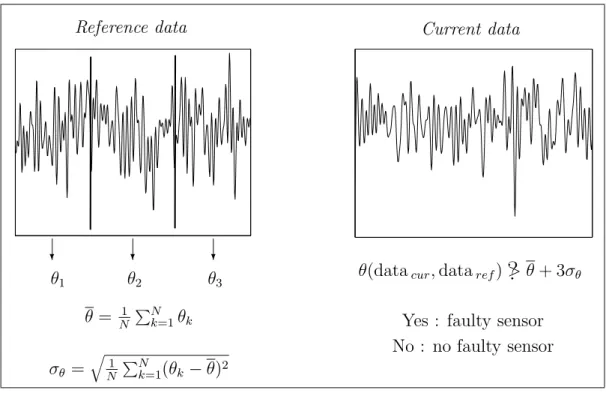
In practice, due to the noise inherent in a measurement process, the largest angle between the subspaces spanned by the reference and current data will not be exactly zero even if all sensors are functioning correctly. Before applying the sensor validation process, the reference data is thus partitioned into several sets. The principal angle between the subspace spanned by each of these sets and the subspace spanned by the whole data set is computed which gives us a collection of different angle values. When dealing with the current data set, an alarm is issued when the monitored angle exceeds the upper control limit (UCL) defined as the mean angle plus three times its standard deviation (see outlier statistics [4]). This corresponds to an 99.7 % confidence interval for a normal distribution. This is illustrated in Figure 1.
When an alert is given, the faulty sensor is then isolated by removing one by one the sensors from both the reference and current data sets. The angle should then be minimum when the faulty sensor is discarded.
Reference data Current data θ1 θ2 θ3 ? ? ? θ = 1 N PN k=1θk σθ = q 1 N PN k=1(θk− θ)2
θ(datacur, dataref) > θ + 3σ
?
θYes : faulty sensor No : no faulty sensor
Figure 1: Comparison of the principal angles of the current and reference data.
SENSOR CORRECTION
Let us suppose that nS sensors are available giving a response vector x(t)
and that for some reason the jth sensor fails. Let us also assume that the er-rant sensor has been identified. If the response given by this sensor contains important information, correction is then necessary. It is first assumed that the reference data set contains enough information to cover normal process opera-tion. The most likely value for the errant sensor is defined as the value which minimises the magnitude of the deviation between the response vector x(t) and its reconstruction ˆx(t). In the approach pioneered by Kramer [5], the reconstruc-tion is performed using non-linear PCA but in this study, we restrict ourselves to linear PCA. Replacement of sensor value thus involves finding the value of xj(t) such that:
minxj J = kx(t) − ˆx(t)k
2
(4) Equation (4) is a univariate optimisation problem. If there is more than one missing sensor at a time, it requires a multivariate approach. It is however interesting to mention that there is an analytical solution to this problem [2]. From a geometric point of view, this procedure amounts to finding the inter-section between a straight line and the subspace spanned by the PCA modes. The straight line is parallel to the axe of the faulty sensor and is defined by the co-ordinates of the remaining sensors.
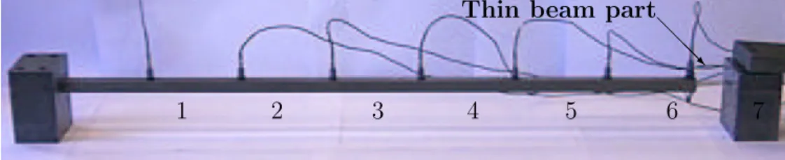
1 2 3 4 5 6 7 Thin beam part
@
@@R
Figure 2: Experimental set-up.
EXPERIMENTAL APPLICATION
Description of the Experimental Structure
The benchmark is similar to the one proposed by the Ecole Centrale de Lyon (France) in the framework of COST Action F3 working group on ”Identification of non-linear systems”. This experimental application involves a clamped steel beam with a thin beam part at the end of the main beam (cf. Figure 2).
Seven accelerometers which span regularly the beam are used to measure the response. The excitation force provided by an electrodynamic shaker is a white-noise sequence band-limited in the 0-500 Hz range. An interesting feature is that, if the structure may be assumed to be linear for low excitation levels, it is no longer the case for higher levels. Indeed, if the excitation level is increased, the thin part is excited in large deflection and a geometrical non-linearity is activated.
Two different kinds of sensor fault are simulated. Firstly, the acceleration measured at the third sensor is multiplied by 1.2 (gain fault). Secondly, it is replaced by a white-noise sequence of the same variance (sensor failure).
Sensor Fault Detection and Isolation REFERENCE DATA
The reference data set contains 70000 points from each of the 7 channels. They correspond to an excitation level equal to 1.4 N for which the structural behaviour is linear. An important thing to check is that there is enough sensors regarding the number of excited mode shapes. The computation of the singular values reveals that two singular values are zero which ensures enough redundancy in the data set.
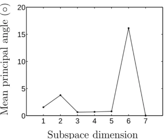
The next step is to estimate the UCL. To this end, the data is partitioned into 28 different sets containing 2500 points each which gives us a collection of 28 different angle values. Figure 3 shows the average value as a function of the subspace dimension. This graph is used for choosing the appropriate subspace dimension. For 7 PCA modes, the angle is exactly zero which is expected because the data is 7-dimensional. Obviously, it is not recommended to choose this number of modes. It is decided to keep 3 PCA modes in the analysis since the
1 2 3 4 5 6 7 0 5 10 15 20 Mean principal angle (◦ ) Subspace dimension
Figure 3: Mean principal angle vs. number of retained PCA modes.
angle is near zero. In addition, they capture almost 99 % of the energy. For a three-dimensional subspace, an alarm will thus be issued when the monitored angle will exceed the following angle (in degree):
U CL3 = 0.65 + 3 ∗ 0.46 = 2.03 (5)
CURRENT DATA
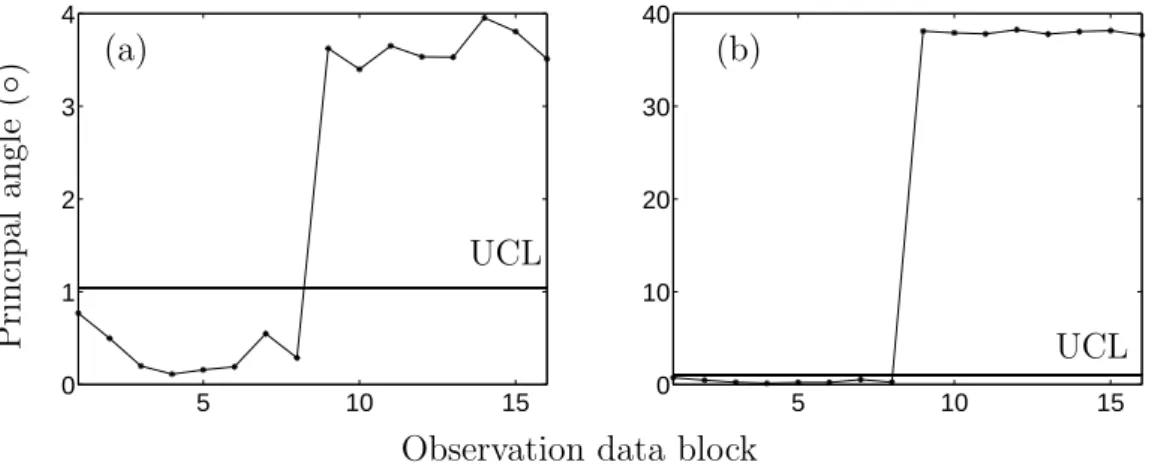
The current data set contains 40000 points whose the last 20000 correspond to a sensor fault. The current data set is partitioned into 16 different sets containing 2500 points each. Figure 4 displays the principal angle between the subspace spanned by each of these sets and the subspace spanned by the whole reference set for both sensor faults. As well for the gain fault as for the sensor failure, it can be observed that the first 20000 points are well below the UCL whereas this is no longer the case for the remainder of the data set. Note that the sensor failure is much easier to identify than the gain fault.
Now that an alarm has been issued, the faulty sensor needs to be identified using the methodology described previously. Figure 5 presents all the angles obtained when the sensors are removed one by one. For both faults, it clearly appears that the angle approaches zero when the third sensor is removed. NON-LINEAR BEHAVIOUR
The whole procedure has also been tested when the reference data set corre-sponds to an excitation level for which the system is non-linear (22 N). Surpris-ingly enough, the results obtained were satisfactory as well. This is expected as long as the excitation level remains the same for both the reference and current data. For instance, the results of the detection stage are shown in Figure 6.
5 10 15 0 1 2 3 4 5 6 7 5 10 15 0 10 20 30 40 50 60 Principal angle (◦ )
Observation data block UCL
UCL
(a) (b)
Figure 4: Monitored angle. (a) Gain fault; (b) sensor failure.
2 4 6 8 0 2 4 6 8 10 2 4 6 8 0 10 20 30 40 50 60 Principal angle (◦ )
Observation data block
(a) (b)
Sensor 3 removed Sensor 3 removed
@@R
@@R
Figure 5: Results of the isolation stage. (a) Gain fault; (b) sensor failure.
5 10 15 0 1 2 3 4 5 10 15 0 10 20 30 40 Principal angle (◦ )
Observation data block UCL
UCL
(a) (b)
Figure 6: Monitored angle for a non-linear structural behaviour. (a) Gain fault; (b) sensor failure.
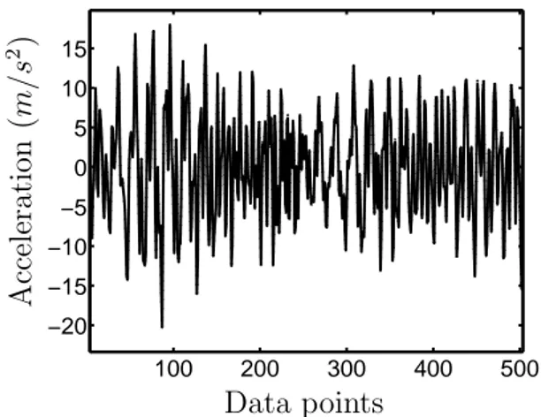
100 200 300 400 500 −20 −15 −10 −5 0 5 10 15 Acceleration (m/s 2 ) Data points
Figure 7: Sensor correction (linear behaviour). Solid line: original response; dotted line: reconstructed response.
Sensor Correction
Now that the third sensor has been declared as faulty, the next step is to retrieve its original response. As underlined in the previous section, we have at our disposal 70000 reference data points. First, the optimum number of retained PCA modes is determined using a sort of cross-validation. More precisely, the response of the third sensor for the last 20000 reference points is predicted using equation (4) and the modes of the first 50000 reference points. The number of modes which gives the minimum mean-square error (MSE) is then selected. This procedure suggests to consider 5 PCA modes.
The reconstructed response of the faulty sensor is now compared to its orig-inal response in Figure 7. 20000 points were faulty but for the sake of clarity only 500 points are represented. It can be observed that both curves agree to the point where the difference between them is not visible (MSE=0.04 %).
It should be noted that the results of the sensor correction in the case of non-linear behaviour are almost as accurate as in the case of linear behaviour (MSE=0.18 % vs. MSE=0.04 %)
CONCLUDING REMARKS
The object of the present paper was to explore the use of PCA for sensor fault detection, isolation and correction. For each of these three objectives, reasonable consistency and accuracy has been observed on an experimental application. Furthermore, the procedure also seems to work well when dealing with non-linear structural behaviour provided that the excitation level is approximately the same for both the reference and current data.
In order to integrate this approach in the framework of structural health monitoring, one has still to be able to discriminate between a sensor fault and a structural damage. This issue will be carefully investigated in future work.
ACKNOWLEDGMENTS
The author G. Kerschen is supported by a grant from the Belgian National Fund for Scientific Research (FNRS) which is gratefully acknowledged.
REFERENCES
[1] Friswell, M., and D.J. Inman. 1999. ”Sensor Validation for Smart Structures,” Journal of Intelligent Material Systems and Structures, 10: 973-982.
[2] Worden, K. 2003. ”Sensor Validation and Correction Using Auto-Associative Neu-ral Networks and Principal Component Analysis,” in International Modal Analysis Conference XXI, Orlando.
[3] De Boe, P., and J.C. Golinval. 2003. ”Principal Component Analysis of a Piezo-Sensor Array for Damage Localization,” Structural Health Monitoring, 2: 137-144. [4] Worden, K., G. Manson, and N.R. Fieller. 2000. ”Damage Detection Using Outlier Analysis,” Journal of Sound and Vibration, 229: 647-667.
[5] Kramer, M.A. 1992. ”Autoassociative Neural Networks,” Computers and Chemical Engineering, 16: 313-328.