Classification of load forecasting studies by forecasting problem to select load
forecasting techniques and methodologies
Jonathan Dumasa,∗, Bertrand Corn´elussea
aUniversity of Li`ege, Department of computer science and electrical engineering, Belgium
Abstract
The key contribution of this paper is to propose a classification into two dimensions of the load forecasting studies to decide which forecasting tools to use in which case. This classification aims to provide a synthetic view of the relevant forecasting techniques and methodologies by forecasting problem. In addition, the key principles of the main techniques and methodologies used are summarized along with the reviews of these papers.
The classification process relies on two couples of parameters that define a forecasting problem. Each article is classified with key information about the dataset used and the forecasting tools implemented: the forecasting tech-niques (probabilistic or deterministic) and methodologies, the data cleansing techtech-niques, and the error metrics.
The process to select the articles reviewed in this paper was conducted into two steps. First, a set of load forecasting studies was built based on relevant load forecasting reviews and forecasting competitions. The second step consisted in selecting the most relevant studies of this set based on the following criteria: the quality of the description of the forecasting techniques and methodologies implemented, the description of the results, and the contributions.
This paper can be read in two passes. The first one by identifying the forecasting problem of interest to select the corresponding class into one of the four classification tables. Each one references all the articles classified across a forecasting horizon. They provide a synthetic view of the forecasting tools used by articles addressing similar forecasting problems. Then, a second level composed of four Tables summarizes key information about the forecasting tools and the results of these studies. The second pass consists in reading the key principles of the main techniques and methodologies of interest and the reviews of the articles.
Word count: 20, 000. Highlights
• A two-dimensional classification of load forecasting studies taking into account the system size
• A classification and a review with key information about the forecasting tools implemented and the dataset used • A way to select the relevant forecasting tools based on the definition of a forecasting problem
• A description of the main forecasting tools: the forecasting techniques and methodologies, the cleansing data techniques and the error metrics
Keywords: load forecasting, classification, forecasting techniques, forecasting methodologies, data cleansing techniques
1. Introduction
Load forecasting arises in a wide range of applications such as providing demand response services for distribution or transmission system operators, bidding on the day ahead or future markets, power system operation and planning, or
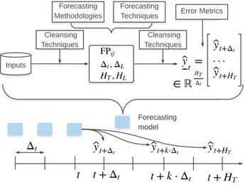
energy policies. Each application is specific and requires a dedicated load forecasting model made of several modules, as depicted in Figure 1. The methodology to build a forecasting model is similar to the one required to solve a data science problem. The first step consists in understanding and formulating the problem: what is the application? What are the targets? This step should determine the forecasting horizon HT, the temporal resolution∆t, the system size HL, and the spatial resolution∆Lof the forecasting model. The second step consists in identifying, collecting, cleaning, and storing the data. The exploration and the analysis of the data are prerequisites for the next step to identify the relevant forecasting tools, the forecasting technique (FT), and the forecasting methodology (FM). The last step is the identification of the Error Metrics (EM) to assess the forecast vectorby
t. Inputs Forecasting Methodologies Forecasting model Cleansing Techniques Cleansing Techniques Error Metrics Forecasting Techniques
Figure 1: Forecasting model and process.
As mentioned above, the identification and selection of the relevant forecasting tools is problem dependent. Al-though the load forecasting literature is composed of several review papers, it is difficult to identify similar forecasting problems as there is no standard problem classification. However, most of the time the forecasting processes are clas-sified based on the forecasting horizon, from very short-term to long-term, and by their deterministic or probabilistic nature. Tzafestas and Tzafestas [1] review four classes of machine learning techniques for short-term load forecasting. Alfares and Nazeeruddin [2] review nine forecasting techniques and mentioned the horizon based classification but did not use it. Hong and Fan [3] review probabilistic forecasting across all forecasting horizons, and provide an overview of representative load forecasting techniques, methodologies and criteria to evaluate probabilistic forecasts. The spa-tial dimension is mentioned in the introduction with hierarchical load forecasting from the household level to the corporate level, across all forecasting horizons. However, it is considered as a separated topic and the spatial criterion is not combined with the horizon criterion. Van der Meer et al. [4] review the probabilistic load and PV forecasting techniques and performance metrics by using the forecasting horizon criterion. One of the objectives of this review is to find a common ground between probabilistic load and PV forecasting to address the problem of net demand forecasting. Deb et al. [5] review nine popular forecasting techniques and hybrid models, consisting in combination of two or more of these techniques, for load forecasting. A qualitative and quantitative comparative analysis of these techniques is conducted. The comparison of the pros and cons for each technique and the summary of the novelties brought by the hybrid models are useful to assess their potential. However, there is no classification across temporal
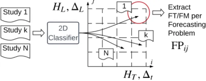
resolution. Each study reviewed is classified into a forecasting problem with key information about the forecasting tools implemented and the dataset used as shown on Figure 2.
2D Classifier Study 1 N Extract FT/FM per Forecasting Problem k 1 Study k Study N
Figure 2: Two-dimensional classifier.
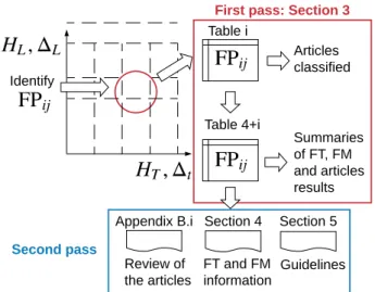
The methodology to use this review is described in Figure 3. When the forecasting problem has been identified, it is possible to select the corresponding class FPi j, 1 ≤ i, j ≤ 4 and to refer to the corresponding classification Table i. With i= 1, 2, 3, 4 corresponding to very short, short, medium, and long-term forecasting. Table i references all the articles classified across the forecasting horizon class considered i with the names of the forecasting techniques and methodologies used. It provides a synthetic view of the forecasting tools used by articles tackling similar forecasting problems. Then, Table 4+ i summarizes key information about the forecasting tools and the results of these studies. Finally, Appendix B.i provides the review of these studies.
The more studies are classified the more forecasting techniques and methodologies are extracted by forecasting problem and the easier it should be to select the relevant ones. Indeed, more and more relevant techniques and methodologies should arise naturally from a given forecasting problem. The process to select the articles reviewed in this paper was conducted into two steps. First, a set of load forecasting studies was built based on relevant load forecasting reviews such as Hong and Fan [3], Van der Meer et al. [4], Deb et al. [5], and forecasting competitions such as the Global Energy Forecasting Competitions 2012 and 2014 [6, 7]. These competitions are valuable sources to compare forecasting results from several combinations of forecasting techniques and methodologies as the forecasting problems and the datasets are the same for all the participants. The second step consisted in selecting the most relevant studies of this set based on the following criteria: the quality of the description of the forecasting techniques and methodologies implemented, the description of the results and the contributions. Figure 4b provides an overview of the articles classified by forecasting problem. However, almost half of the articles are classified within short and medium-term horizons for small load system. These articles are the top entries of the Global Energy Forecasting Competitions 2012 and 2014. Long-term horizon and medium load system classes have received less interest in the literature. This paper aims at providing a synthetic view of the relevant forecasting tools for a given forecasting problem, and the classification process was limited to keep the document readable. A possible extension is discussed in the conclusion.
This review has three main objectives: classifying the load forecasting studies of the literature into two dimen-sions leading to a set of sixteen classes; providing for each forecasting problem FPi ja synthetic view of the relevant forecasting tools (forecasting techniques and methodologies); ease the selection of the relevant forecasting tools to use in which case.
The paper structure is in line with the methodology depicted in Figure 3. Section 2 defines the time and load couples’ classification parameters to build the classifier. Section 3 classifies the reviewed articles by forecasting problem. Tables 1, 2, 3 and 4 provide a synthetic view of the forecasting tools implemented and the datasets used for each article classified. Tables 5, 6.1, 6.2, 7.1, 7.2, and 8 summarize key information about the forecasting tools and the results. Section 4 focuses on the forecasting tools. The forecasting techniques and the methodologies implemented in the articles reviewed are succinctly summarized and references are given for further details. Finally, Section 5 proposes general guidelines. Notations are provided in Appendix A. The reviews of the studies are in Appendix B. The datasets, data cleansing techniques, and error metrics used are referenced in Appendix C, Appendix D, and Appendix E.
Table i Articles classified Table 4+i Summaries of FT, FM and articles results Identify Appendix B.i Review of the articles Section 4 FT and FM information Section 5 Guidelines
First pass: Section 3
Second pass
Figure 3: Methodology to use this review.
2. Load forecasting problem definition
The following subsections define the parameters of a load forecasting problem.
2.1. Temporal forecasting horizon HT
Hong and Fan [3] proposed a classification based on the forecast horizon into four categories: very short-term load forecasting (VSTLF), short-term load forecasting (STLF), medium-term load forecasting (MTLF), and long-term load forecasting (LTLF). The cut-off horizons are one day, two weeks, and three years respectively. The cut-off motivations are provided by Hong et al. [8] and based on weather, economics and land use information.
The one-day cut-off between very short and short-term load forecasting is related to the temperature sensibility. In very short-term load forecasting, the temperature is relatively stable as the horizon is from a few hours to maximum one day. Thus, load is assumed to be weakly impacted by the temperature and can be forecasted only by its past values. However, depending on the system temperature load sensitivity this cut-off can be discussed. The two weeks cut-off between short and medium-term load forecasting is related to the temperature forecasts unreliability above this horizon. In short-term load forecasting, load is assumed to be affected significantly by the temperature. However, as in very short-term load forecasting, both economics and land use information are relatively stable within this horizon and are not necessarily required. The three years cut-off between medium- and long-term load forecasting is related to the economics forecasts unreliability above this horizon. In medium-term load forecasting, economics is required and predictable, temperature is simulated as no forecasts are reliable and land use is optional as it is stable within this horizon. In long-term load forecasting, temperature and economics are simulated and land use forecasts are used. Above a horizon of five years land use forecasts become unreliable and are simulated.
A cut-off is always questionable as it depends on the system considered and the forecast application. For large systems such as states or regions, forecasts with horizons up to a few years depend on macroeconomic indicators (such as gross domestic product). However, smaller systems, such as microgrids or small industries, depend on other economic indicators with shorter horizons. The choice of a one-year cut-off between medium and long-term load
(HT, ∆t) (HL, ∆L) VSTLF HT≤ 1 d ∆t≤ 1 h STLF HT≤ 2 w ∆t≤ 1 h MTLF HT≤ 1 y ∆t≤ 1 d LTLF 1 y≤ HT ∆t≤ 1 y VSLS HL<1 MW ∆L < 1 kW SLS HL≤1 GW ∆L≤ 1 MW MLS HL≤10 GW ∆L≤ 1 MW LLS 10 GW≤ HL ∆L≤ 1 GW
(a) Classes of the two-dimensional classifier.
VSTLF STLF MTLF LTLF LLS MLS SLS VSLS 3 3 1 1 0 0 2 1 1 6 9 2 2 2 1 0 1 2 3 4 5 6 7 8 9 10 number of articles
(b) Articles classified by forecasting problem. Figure 4: Classification of load forecasting studies.
The temporal forecasting resolution ranges from a few minutes to years depending on the forecasting horizon. Usually the smaller horizon, the smaller the resolution is. Typical values are: from minutes to hours for very short-term load forecasting and short-short-term load forecasting, from hours to days for medium-short-term load forecasting and from days to years for long-term load forecasting.
2.3. Load system size HL
The load system size is related to the load capacity of the system considered. It is possible to classify a load system into four categories: very small load system (VSLS), small load system (SLS), medium load system (MLS) and large load system (LLS). Very small load systems are residential areas, small industrials or microgrids with load values from a few kW to MW, small load systems are thousands of residential areas, large industrials or microgrids from a few MW to GW, medium load systems are regional or small state grids from a few GW to ten GW, and large load systems are large state to continental grids from ten GW to a hundred GW.
2.4. Load forecasting resolution∆L
The load forecasting resolution is the resolution of the forecasts. Usually, the smaller the load system size, the smaller the load resolution is. Typical values are from W to kW for very small load system, kW to MW for small load system and medium load system, MW to GW for large load system.
2.5. A two-dimensional classification process
The four parameters HT,∆t, HLand∆Ldefine a four dimensional classifier. However, as∆tis related to HT and ∆Lto HL, it is possible to define a two-dimensional classifier by considering the temporal and load couples (HT, ∆t) and (HL, ∆L) denoted by the integers i and j, respectively. Figure 4a shows the sixteen forecasting problems defined by this classifier. With i= 1, 2, 3, 4 corresponding to very short, short, medium, and long-term forecasting. And with
3. Two-dimensional load forecasting classification
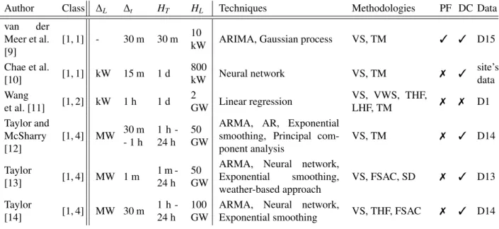
Figure 4b provides a synthetic view of the classification by forecasting problem of the reviewed articles, according to the selection process explained in the introduction1. Tables 1, 2, 3, and 4 correspond to very short, short, medium, and long-term forecasting, respectively. They provide a synthetic view of the forecasting tools and datasets used. Within each table the studies are classified from top to bottom by increasing the system size. The information provided are the references, the classes [i, j], the values of∆L,∆t, HT and HL, the names of the forecasting techniques and methodologies, data cleansing techniques, error metrics, and the datasets used. Tables 5, 6.1, 6.2, 7.1, 7.2, and 8 summarize key information about the forecasting tools and the results. Appendix B.1 to Appendix B.4 provide the review of these papers. Tables 9.1, 9.2, 10, 11.1, and 11.2 in Appendix C, Appendix D, and Appendix E provide key information about the datasets, data cleansing techniques and error metrics used.
Table 1: Very Short-Term Load Forecasting classification.
Author Class ∆L ∆t HT HL Techniques Methodologies PF DC Data
van der
Meer et al. [9]
[1, 1] - 30 m 30 m 10
kW ARIMA, Gaussian process VS, TM 3 3 D15
Chae et al. [10] [1, 1] kW 15 m 1 d 800 kW Neural network VS, TM 7 3 site’s data Wang et al. [11] [1, 2] kW 1 h 1 d 2 GW Linear regression VS, VWS, THF, LHF, TM 7 7 D1 Taylor and McSharry [12] [1, 4] MW 30 m - 1 h 1 h -24 h 50 GW
ARMA, AR, Exponential smoothing, Principal com-ponent analysis VS, TM 7 3 D14 Taylor [13] [1, 4] MW 1 m 1 m -24 h 50 GW
ARMA, Neural network,
Exponential smoothing, weather-based approach VS, FSAC, SD 7 3 D13 Taylor [14] [1, 4] MW 30 m 1 h -24 h 100 GW
ARMA, Neural network,
Table 2: Short-Term Load Forecasting classification.
Author Class ∆L ∆t HT HL Techniques Methodologies PF DC Data
Shepero et al. [15] [2, 1] - 30 m 1 w 10 kW Gaussian process VS 3 3 D15 Ahmad and Chen [16] [2, 1] kW 5 m 1 w -1 M 500 kW
Decision tree, k-nearest
neighbor, linear regression VS 7 3
site’s data
Goude
et al. [17] [2, 2] - 10 m 1 d
50
MW General additive models
VS, LHF, THF, MWS 7 3 D3 Charlton and Sin-gleton [18] [2, 2] kW 1 h 1 w 2 MW Linear regression VS, LHF, THF, MWS, LA, FSAC 7 3 D1 Lloyd [19] [2, 2] kW 1 h 1 w 2 MW
Gradient boosting, Gaussian
process, linear regression VS, FWC, LHF 7 3 D1
Nedellec
et al. [20] [2, 2] kW 1 h 1 w
2 MW
General additive models, Random forest VS, LHF, THF, MWS 7 7 D1 Taieb and Hyndman [21] [2, 2] kW 1 h 1 w 2 MW
Gradient boosting, general additive models LHF, THF, VS, MWS 7 3 D1 Hong et al. [8] [2, 2] kW 1 h 1 h -1 y 1 GW
Linear and Fuzzy interaction
regressions, Neural network VS, THF, TM 7 7 D2
Hong and
Wang [22] [2, 4] MW 1 h 1 d
25 GW
Linear and Fuzzy interaction
regressions VS, TM 7 7 D10 Al-Qahtani and Crone [23] [2, 4] MW 1 h 1 d 50 GW k-nearest neighbor VS, TM 7 7 D13 L´opez et al. [24] [2, 4] MW 1 h 9 d 40 GW Neural network, AR VS, LHF, MWS, FWC, TM 3 3 D5
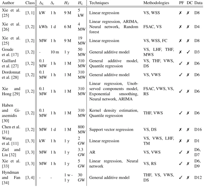
Table 3: Medium-Term Load Forecasting classification.
Author Class ∆L ∆t HT HL Techniques Methodologies PF DC Data
Xie et al. [25] [3, 1] kW 1 h 9 M 5 kW Linear regression VS, WSS 7 7 D8 Xie et al. [26] [3, 2] kWh 1 d 6 M 4 MW
Linear regression, ARIMA,
Neural network, Random
forest FSAC, VS 7 7 D4 Xie et al. [25] [3, 2] MW 1 h 9 M 19 MW Linear regression VS, WSS, FC 7 7 D8 Goude et al. [17] [3, 2] - 10 m 1 y 50
MW General additive model
VS, LHF, THF, MWS 7 3 D3 Gaillard et al. [27] [3, 2] 0.1 MW 1 h 1 M 310 MW
General additive model, Quantile regression VS, THF, VWS, DS 3 7 D6 Dordonnat et al. [28] [3, 2] 0.1 MW 1 h 1 M 310
MW General additive model VS, VWS 3 7 D6
Xie and Hong [29] [3, 2] 0.1 MW 1 h 1 M 310 MW
Linear regression, Unob-served components model,
Exponential smoothing,
Neural network, ARIMA
FSAC, VWS, VS, RS 3 7 D6 Haben and Gi-asemidis [30] [3, 2] 0.1 MW 1 h 1 M 310 MW
Kernel density estimation,
Quantile regression THF, VWS 3 7 D6
Chen et al.
[31] [3, 2] MW 1 d 1 M
800
MW Support vector regression VS, DS 7 7 D16
Wang et al. [11] [3, 3] kW 1 h 1 y 2 GW Linear regression VS, VWS, LHF, TM 7 7 D1 Ziel and Liu [32] [3, 3] MW 1 h 1 y 3.3 GW AR VS, VWS 3 7 D6, D7 Xie et al. [33] [3, 3] MW 1 h 1 y 5 GW
Linear regression, Neural
network VS, RS 3 7 D6, D9 Hyndman and Fan [34] [3, 4] - - 1 w -1 y 30
GW General additive model
THF, VS, VWS,
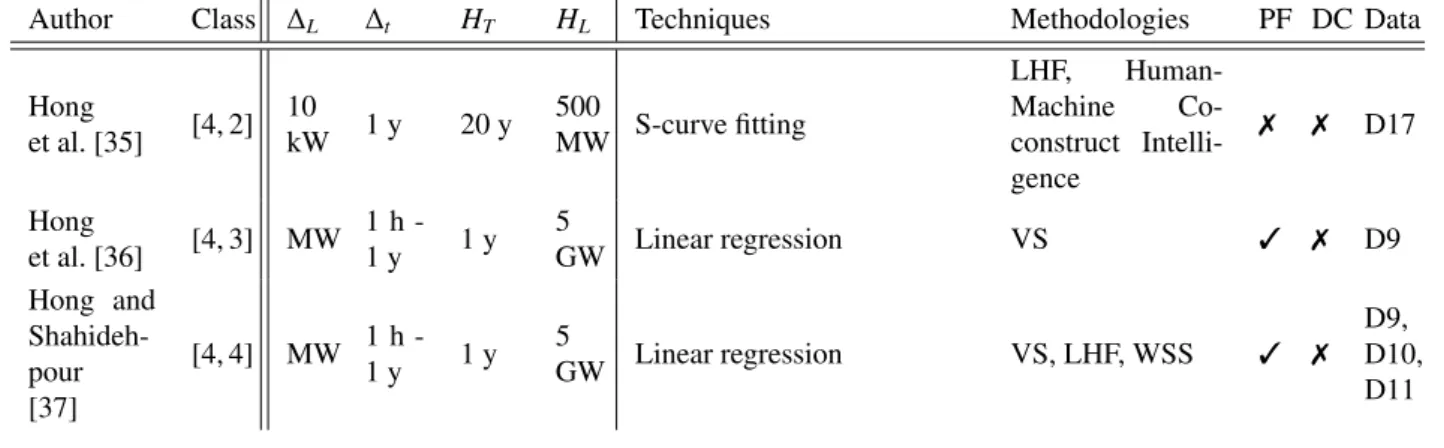
Table 4: Long-Term Load Forecasting classification.
Author Class ∆L ∆t HT HL Techniques Methodologies PF DC Data
Hong et al. [35] [4, 2] 10 kW 1 y 20 y 500 MW S-curve fitting LHF, Human-Machine Co-construct Intelli-gence 7 7 D17 Hong et al. [36] [4, 3] MW 1 h -1 y 1 y 5 GW Linear regression VS 3 7 D9 Hong and Shahideh-pour [37] [4, 4] MW 1 h -1 y 1 y 5 GW Linear regression VS, LHF, WSS 3 7 D9, D10, D11
Table 5: Very Short-Term Load forecasting summary. Author Class Forecasting tools and results
van der
Meer et al. [9]
[1, 1]
Gaussian process is implemented and ARIMA used as benchmark. The dynamic Gaussian pro-cess uses a sliding window training methodology with a linear combination of the squared ex-ponential and Mat´ern kernels. Deterministic and probabilistic metrics are computed using a blocked form of k-fold cross-validation procedure. The Gaussian process models were consis-tently outperformed by ARIMA by a factor in terms of MAPE and NRMSE for the demand, PV production, and net demand forecasting. However, ARIMA produced higher prediction intervals that are constant over time. In contrast, the Gaussian process have wide and narrow prediction intervals between periods of high and low uncertainty.
Chae et al.
[10] [1, 1]
Random forest is used for feature extraction and a feed-forward artificial neural network was selected among nine machine learning techniques. A static, accumulative and sliding window training methodologies are implemented and deterministic metrics are computed using a blocked form of k-fold cross-validation procedure. The average value of the daily coefficient variance of the RMSE, that is a normalized RMSE, of the consumption is around 10 % and the average APE of the daily peak demand is around 5 %.
Wang
et al. [11] [1, 2]
A customized linear regression technique models the recency effect both at the aggregated and bottom levels and for each hour of the day. A static and sliding window training methodologies are used to compute yearly and daily forecasts. The customized linear regression model signif-icantly outperformed the benchmark with a MAPE reduced between 10 % and 20 % depending on the load level and the forecasting horizon.
Taylor and McSharry [12]
[1, 4]
Several statistical univariate methods are implemented: double seasonal ARMA, periodic Au-toregressive, double seasonal Holt-Winters exponential smoothing, intraday cycle exponential smoothing and principal component analysis. A static training methodology is used. The double seasonal Holt-Winters method performed the best followed by the principal component analysis and the seasonal ARMA. The MAPE are between 0.75 % and 2.2 %.
Taylor
[13] [1, 4]
Several statistical univariate methods are implemented: double seasonal ARMA, double seasonal Holt-Winters exponential smoothing, double seasonal intraday cycle exponential smoothing, the weather-based approach used at National Grid, and a combination of the weather-based approach and the double seasonal exponential smoothing by taking the average. A static training method-ology is used. For forecasting horizons between one and thirty minutes, the double seasonal exponential smoothing ranked first with MAPE values between 0.12 % and 0.5 %. For forecast-ing horizons between one minutes and one day, the combination approach performed the best with MAPE values between 0.15 % and 1.2 %.
Taylor
[14] [1, 4]
Extension from double to triple statistical seasonal univariate methods are implemented along with a feed-forward neural network. A combination of the triple seasonal ARMA and Holt-Winter exponential smoothing approaches is also implemented. A static training methodology is used. The triple seasonal versions of all the methods were more accurate than the double ones with MAPE values from 0.4 % to 1.75 %. The combination approach performed the best results.
Table 6.1: Short-Term Load forecasting summary, part 1. Author Class Forecasting tools and results
Shepero
et al. [15] [2, 1]
A log-normal transformation of the data before applying Gaussian process is compared to the conventional Gaussian process approach. The training methodology is a blocked form of cross-validation. The log-normal transformation produced sharper forecasts than the conventional ap-proach and the sharpness of the forecasts varied throughout the day. That is not the case without transformation. However, both approaches were not able to capture the sudden sharp increments of the load.
Ahmad and Chen [16]
[2, 1]
Compact decision trees, fit k-nearest neighbor, linear and stepwise linear regressions models are implemented. The inputs are climate variables, lags of load, and calendar variables. The training methodology is static. The k-nearest neighbor approach achieved the best MAPE with 0.076 % followed by the decision trees for one week ahead forecasting. Inversely, the decision trees performed the best MAPE with 0.044 % followed by the k-nearest neighbor for one month ahead forecasting.
Goude
et al. [17] [2, 2] Refer to Table 7.1 for description.
Charlton
and
Sin-gleton [18]
[2, 2]
A linear regression model with temperature and calendar variables is implemented. Load and temporal hierarchical forecasting methodologies are used by computing a model for each zone, hours of the day, seasons of the year, weekdays, and weekend. A multiple weather station selec-tion methodology computes for each zone a linear combinaselec-tion of the five best weather staselec-tions. Outliers removal is used. Ranked first at the Global Energy Forecasting Competition 2012.
Lloyd [19] [2, 2]
The final model is a weighted average of gradient boosting, Gaussian process, and linear re-gression models. There is a gradient boosting model per zone and the demand is modeled as a function of temperature and calendar variables. The Gaussian process kernels are the squared exponential and the periodic ones. Ranked second at the Global Energy Forecasting Competition 2012.
Nedellec
et al. [20] [2, 2]
A multi-scale approach with three models that correspond to the long, medium, and short terms. General additive models are used for long and medium terms and random forest for short-term. The inputs are the monthly load and temperature, the day type, the time of the year, and a smoothed temperature. There is a model for each load zone and a medium-term model is fit-ted per instant of the day. Ranked third at the Global Energy Forecasting Competition 2012. The short-term model provides an average gain of 5 % in terms of RMSE.
Table 6.2: Short-Term Load forecasting summary, part 2. Author Class Forecasting tools and results
Taieb and Hyndman [21]
[2, 2]
A gradient boosting approach to estimate general additive models. There is a model per load zone and for each hour of the day. Ranked fourth at the Global Energy Forecasting Competition 2012.
Hong
et al. [8] [2, 2]
A systematic approach to investigate short-term load forecasting is conducted. A methodology to select the relevant variables is exposed. Several linear and fuzzy regression models, and single-output feed-forward neural networks with consecutive refinements are implemented. A sliding window methodology is used. The case study demonstrated that linear regression models can be more accurate than feed-forward neural networks and fuzzy regression models given the same amount of input information. The MAPE of the linear regression benchmark and its customized version are approximately 5 % and 3 % for horizons of one hour, one day, one week, two weeks, and one year. The MAPE of the feed-forward neural network benchmark and its customized versions are approximately 6.5 % and 4.5 % for an horizon of one year.
Hong and Wang [22] [2, 4]
A fuzzy interaction regression approach with three refined versions are compared to a linear regression model. A sliding window methodology is used. The most refined version of the fuzzy interaction regression models performed the best MAPE with 3.68 %.
Al-Qahtani and Crone [23]
[2, 4]
A univariate and multivariate k-nearest neighbor approaches are implemented. The training methodology is static. The multivariate approach takes lags of load and calendar variables as inputs. The MAPE of the multivariate and univariate approaches are 1.81 % and 2.38 %.
L´opez
et al. [24] [2, 4]
An on-line real-time hybrid load-forecasting model based on an Autoregressive model and neural networks is studied. The training methodology is static. The final model at the national level is a linear combination of four sub-models. The model takes calendar information such as special days and temperature lags as inputs. The RMSE and MAPE of the final model are 1.83 % and 1.56 %.
Table 7.1: Medium-Term Load forecasting summary, part 1. Author Class Forecasting tools and results
Xie et al.
[25] [3, 1]
The linear regression benchmark of Hong et al. [8] is used as a starting model. Then, the variable selection framework of Hong et al. [8] is applied to customized the model. The training method-ology is static. The customized linear regression model forecasts the load per customer. The survival analysis model forecasts the tenured customers. Then, the final forecast is the multipli-cation of both previous forecasts. This methodology is validated through a field implementation at a fast growing U.S. retailer. The MAPE of the customized linear regression model is 11.56 %. The MAPE of the final forecast is around 10.5 %.
Xie et al.
[26] [3, 2]
A combination of four forecasting techniques is implemented: linear regression, ARIMA, feed-forward neural network, and random forest. A feed-forward and a backward selection strategies are used to select the relevant variables of the linear regression model. The training methodology is static. This methodology ranked third at NPower Forecasting Challenge 2015. The MAPE of the final model is 2.40 % and better than any of the individual model. The best linear regression model performed 2.47 %, the neural network 3.27 %, the random forest 3.87 %, and ARIMA 8.23 %.
Xie et al.
[25] [3, 2] Refer to [3, 1] of this Table for description.
Goude
et al. [17] [3, 2]
A general additive model is implemented for one day ahead forecasting and two others for one year ahead forecasting. The training methodology is static. Load and temporal hierarchical forecasting methodologies are used. These models are able to forecast more than 2 000 electricity consumption series. The one day ahead model achieved a median MAPE of 5 %. The one year ahead models achieved a median MAPE of 6 % and 8 %.
Gaillard
et al. [27] [3, 2]
A concatenation of a short and medium-term quantile generalized additive models is imple-mented. Temperature scenarios are used into the probabilistic forecasting load model. A weather station selection is used to compute an average temperature that is an input of the models. There is one model fitted per hour of the day. Ranked first at the Global Energy Forecasting Competi-tion 2014. The PLF values are between 4 and 11.
Dordonnat et al. [28] [3, 2]
A temperature based deterministic load model with a generalized additive model uses tempera-ture sample paths to produce load paths. The final probabilistic forecast is derived from these final paths. A weather station selection is used to compute an average temperature as input of the model. Ranked second at the Global Energy Forecasting Competition 2014. The MAPE values of the deterministic model are between 8.74 % and 11.83 %. The PLF of the probabilistic models are between 7.37 to 8.37.
Table 7.2: Medium-Term Load forecasting summary, part 2. Author Class Forecasting tools and results
Xie and
Hong [29] [3, 2]
An integrated solution with pre-processing, forecasting, and post-processing is proposed. The pre-processing is data cleansing and temperature weather station selection. The forecasting part is achieved with a linear regression deterministic model combined with residual forecasts of four techniques: exponential smoothing, ARIMA, feed-forward neural network, and unobserved components model. Then, temperature scenarios are used to generate probabilistic forecasts. Fi-nally, the post-processing uses residual simulation to improve the probabilistic forecasts. Ranked third at the Global Energy Forecasting Competition 2014. The residual simulation of the post-processing step helped to improve the forecasts. The PLF of the submitted model are between 3.360 and 11.867. Haben and Gi-asemidis [30] [3, 2]
A hybrid model of kernel density estimation and quantile regression is implemented. It relies on a combination of five models each one forecasting on a dedicated time period. Ranked fourth at the Global Energy Forecasting Competition 2014.
Chen et al.
[31] [3, 2]
A support vector regression model using data segmentation is implemented. It demonstrates that a conservative approach using only available correct information is recommended in this case due to the difficulty to provide accurate temperature forecast. Ranked first at the EUNITE Competition 2001.
Wang
et al. [11] [3, 3] Refer to Table 5 for description.
Ziel and
Liu [32] [3, 3]
A methodology based on Least Absolute Shrinkage and Selection Operator (LASSO) and bivari-ate time-varying threshold Autoregressive model. The LASSO has the properties of automati-cally selecting the relevant variables of the model. Then, a residual-based bootstrap is used to simulate future scenario sample paths to generate probabilistic forecasts. Ranked second at the extended version of the Global Energy Forecasting Competition 2014. The PLF scores are 7.44 and 54.69 for both competitions.
Xie et al.
[33] [3, 3]
Three linear regression models and three feed-forward neural networks are implemented with an increasing number of input features. Then, the probabilistic forecasts are computed by generating weather scenarios. Residual simulation based on normality assumption is used to improve the probabilistic forecasts. The improvement provided by residual simulation is diminishing with the refinement of the underlying model. A very comprehensive underlying model will not benefit from residual simulation based on the normality assumption.
Hyndman
and Fan
[34]
[3, 4]
A methodology to forecast the probability distribution of annual, seasonal and weekly peak elec-tricity demand and energy consumption for various regions of Australia is proposed. The final model is the combination of a short and long-term models. The forecast distributions are derived from the model using a mixture of temperature and residual simulations, and future assumed demographic and economic scenarios. Unfortunately, there is no quantitative metric used in this study. However, the twenty-six actual weekly maximum demand values fall within the region predicted from the ex-ante forecast distribution.
Table 8: Long-Term Load forecasting summary. Author Class Forecasting tools and results
Hong
et al. [35] [4, 2]
A forecasting model is composed of a bottom-up and top-down modules. The first one aggregates load for each small area in each level to produce the S-curve parameters. Then, the second one takes these parameters as inputs to allocates the utility’s system forecast from the top to the bottom level. A human expert is integrated into the problem solving loop to improve the results from this automated approach. The proposed method has been applied to several utilities and has received satisfactory results.
Hong
et al. [36] [4, 3]
An approach based on linear regression models that takes advantage of hourly information com-putes long-term probabilistic load forecasts. The short-term load models of Hong et al. [8] are extended to long-term forecasting by adding the Gross State Product macroeconomic indica-tor. The probabilistic forecasts are computed by using weather and macroeconomic scenarios. Weather normalization is applied to estimate the normalized load profile. A sliding window methodology is used. The customized short-term models performed a MAPE of 4.7 % for one year ahead forecasting.
Hong and Shahideh-pour [37]
[4, 4]
A review of load forecasting topics and three case studies based on linear regression for long-term load forecasting are exposed. The main effects of the linear regression models are the temperature modeled by a third order polynomial, the calendar variables, and a macro economic indicator. The cross effects are several cross variables of temperature and calendar variables. These case studies are exposed to assist Planning Coordinators to provide a real-world demonstration.
4. Load forecasting tools
This paper adopts the distinction made by Hong and Fan [3] between the forecasting techniques and methodolo-gies. A forecasting technique is a group of models that fall in the same family, such as linear regression and artificial neural networks, etc. A forecasting methodology is a framework that can be implemented with multiple forecasting techniques. Subsections 4.1, 4.2, Appendix D, and Appendix E provide some information and references about the forecasting techniques, methodologies, data cleansing techniques and error metrics implemented in the articles reviewed.
4.1. Forecasting techniques
4.1.1. Basic notions of supervised learning
Friedman et al. [38] provide useful details and explanations about supervised learning algorithms, model assess-ment and selection. A load forecasting problem is a supervised learning regression problem. In supervised learning, the goal is to predict the value of an outcome measure based on a number of input measures. Supervised learning is opposed to unsupervised learning, where there is no outcome measure, and the goal is to describe the associations and patterns among a set of input measures. A symbolic output leads to a classification problem whereas a numerical output leads to a regression problem. In the statistical literature, the inputs are often called the predictors and more classically the independent variables. In the pattern recognition literature, the term features is preferred. Both terms, predictors or features are used in this paper.
There are three main criteria to compare and select learning algorithms. The accuracy, measured by the gener-alization error. It is estimated by efficient sample re-use such as cross-validation or bootstrapping. The efficiency which is related to the computation time and scalability for learning and testing. The interpretability related to the comprehension brought by the model about the input-output relationship. Unfortunately, there is usually a trade-off between these criteria.
4.1.2. Forecasting techniques implemented
This subsection provides the basic principles and some references of the forecasting techniques implemented in the articles reviewed. Figure 5 shows for each forecasting technique in the articles reviewed a heat map with the
VSTLF STLF MTLF LTLF LLS MLS SLS VSLS 1 1 0 0 0 0 1 0 0 1 2 0 1 0 0 0 Neural network VSTLF STLF MTLF LTLF LLS MLS SLS VSLS 3 1 0 0 0 0 1 0 0 0 2 0 1 0 0 0 ARIMA VSTLF STLF MTLF LTLF LLS MLS SLS VSLS 3 0 0 0 0 0 0 0 0 0 1 0 0 0 0 0 Exponential smoothing VSTLF STLF MTLF LTLF LLS MLS SLS VSLS 0 1 0 0 0 0 0 0 0 1 0 0 0 0 0 0
Fuzzy interaction regression 1.0 1.5 2.0 2.5 3.0 1.0 1.5 2.0 2.5 3.0 1.0 1.5 2.0 2.5 3.0 1.0 1.5 2.0 2.5 3.0 VSTLF STLF MTLF LTLF LLS MLS SLS VSLS 0 0 1 0 0 0 0 0 0 3 3 0 0 0 0 0
General additive models
VSTLF STLF MTLF LTLF LLS MLS SLS VSLS 0 0 0 0 0 0 0 0 0 1 0 0 0 1 0 0 Gaussian process VSTLF STLF MTLF LTLF LLS MLS SLS VSLS 0 0 0 0 0 0 1 0 0 3 0 0 1 0 0 0
Gradient boosting, Random forest
VSTLF STLF MTLF LTLF LLS MLS SLS VSLS 0 0 0 0 0 0 0 0 0 0 1 0 0 0 0 0
Kernel density estimation 1.0 1.5 2.0 2.5 3.0 1.0 1.5 2.0 2.5 3.0 1.0 1.5 2.0 2.5 3.0 1.0 1.5 2.0 2.5 3.0 VSTLF STLF MTLF LTLF LLS MLS SLS VSLS 0 1 0 0 0 0 0 0 0 0 0 0 0 1 0 0 k-NN VSTLF STLF MTLF LTLF LLS MLS SLS VSLS 0 1 0 1 0 0 2 1 0 3 3 0 1 1 0 0 Linear regression VSTLF STLF MTLF LTLF LLS MLS SLS VSLS 0 0 0 0 0 0 0 0 0 0 2 0 0 0 0 0 Quantile regression VSTLF STLF MTLF LTLF LLS MLS SLS VSLS 0 0 0 0 0 0 0 0 0 0 1 0 0 0 0 0
Support vector regression 1.0 1.5 2.0 2.5 3.0 1.0 1.5 2.0 2.5 3.0 1.0 1.5 2.0 2.5 3.0 1.0 1.5 2.0 2.5 3.0
Figure 5: Load forecasting techniques by forecasting problem.
number of implementations by forecasting problem. Without surprising, linear regression, neural networks, gradient boosting and ARIMA are the techniques the most implemented. However, for specific forecasting problems some techniques are more used than other such as exponential smoothing for the class [1, 4].
Artificial neural network.
Artificial neural network basic principles are discussed in Friedman et al. [38] and Weron [39] did a useful review of the various neural network techniques. The artificial neural network is a supervised learning method initially inspired by the behavior of the human brain and consists of the interconnection of several small units. The motivations for neural networks dates back to McCulloch and Pitts [40] and now the term neural network has evolved to encompass a large class of models and learning methods.
The central idea of artificial neural network is to extract linear combinations of the inputs as derived features, and then model the target as a nonlinear function of these features. The neural network has unknown parameters,
model that takes into account the random nature and time correlations of the phenomenon under study is the Autore-gressive Moving Average model (ARMA). It assumes the stationary of the time series under study. As the electricity demand is non-stationary the ARMA models are not always suitable and a transformation of the series to the sta-tionary form is done by differencing. Autoregressive Integrated Moving Average (ARIMA) or Box-Jenkins model, introduced by Box et al. [41], is a general model that contained both AR and MA parts and explicitly included dif-ferencing in the formulation that are often used for load forecasting. ARX, ARMAX, ARIMAX and SARIMAX are generalized counterparts of AR, ARMA, ARIMA and SARIMA taking into account exogenous variables such as weather or economic.
Ensemble methods.
Friedman et al. [38] discuss ensemble methods. The idea is to build a prediction model by combining the strengths of a collection of simpler base models to change the bias variance trade-off. Ensemble methods can be classified into two categories: the averaging and the boosting techniques. The averaging techniques build several estimators independently and then average out their predictions, reducing therefore the variance from a single estimator. Bagging and random forest techniques are part of this family. The boosting techniques involve the combination of several weak models built sequentially. AdaBoost and gradient tree boosting methods fall into this category. The averaging techniques decrease mainly variance whereas boosting technique decreases mainly bias.
Exponential smoothing.
Gardner Jr [42] brings the state of the art in exponential smoothing up to date since Gardner Jr [43]. The equations for the standard methods of exponential smoothing are given for each type of trend. Exponential smoothing assigns weights to past observations that decrease exponentially over time. Hyndman et al. [44] classified fifteen exponential smoothing models versions based on the trend and seasonal components: additive, multiplicative, etc.
Fuzzy interaction regression.
Asai et al. [45] did the earliest formulation of fuzzy regression analysis. Hong and Wang [22] define the fundamental difference between the linear regression and fuzzy interaction regression assumptions as the deviations between the observed values and the estimated values. In linear regression, these values are supposed to be errors in measure-ment or observations that occur whereas they are assumed to depend on the indefiniteness of the system structure in fuzzy interaction regression. Hong and Wang [22], Asai et al. [45] and Tanaka et al. [46] provide useful details and explanations about fuzzy interaction regression theoretical background.
Generalized additive models.
Generalized additive models allow the use of nonlinear and nonparametric terms within the framework of additive models and are used to estimate the relationship between the load and explanatory variables such as temperature and calendar variables. According to Friedman et al. [38], the most comprehensive source for generalized additive models is Hastie and Tibshirani [47]. Efron and Tibshirani [48] provide an exposition of modern developments in statistics for a nonmathematical audience. Generalized additive models are a useful extension of linear models, making them more flexible while still retaining much of their interpretability.
Gradient boosting.
Boosting techniques are part of ensemble methods and discussed by Friedman et al. [38], B¨uhlmann et al. [49] and Schapire and Freund [50]. The motivation for boosting is a procedure that combines the outputs of many weak learners to produce a powerful committee. Schapire [51] showed that a weak learner could always improve its performance by training two additional classifiers on filtered versions of the input data stream. Thus, the purpose of boosting is to sequentially apply the weak classification algorithm to repeatedly modified versions of the data, thereby producing a sequence of weak classifiers. Then, the predictions from all of them are combined through a weighted majority vote to produce the final prediction. Boosting regression trees such as Multiple Additive Regression Trees (MART) improves their accuracy often dramatically. However, boosting is more sensitive to noise than averaging techniques (bagging, random forest) and reduces the bias but increases the variance.
Gaussian process and Log-normal process.
Rasmussen [52] defines a Gaussian process as ”a collection of random variables, any finite number of which have joint Gaussian distributions”. It is fully specified by its mean and covariance functions. This is a natural generalization of the Gaussian distribution whose mean and covariance is a vector and matrix, respectively. The Gaussian distribution is over vectors, whereas the Gaussian process is over functions. The covariance functions, or kernels, encode the relationship between the inputs. The forecasting accuracy is strongly dependent on the kernels selection. Rasmussen [52] provide a detailed presentation of Gaussian process and their related kernels.
Log-normal process is derived from conventional Gaussian process by performing the logarithm of the normalized load data. Based on the Ausgrid residential dataset (D15), Shepero et al. [15] noticed that the probability distribu-tion of the load is not normally distributed, but is positively skewed and seems to follow a log-normal distribudistribu-tion. Munkhammar et al. [53] did a similar study based on a residential load dataset by using the Weibull and the log-normal distributions. Thus, depending on the load data distribution, modeling the residential load by a log-normal distribution might provide better results than applying directly Gaussian process.
Kernel density estimation.
Kernel density estimation is a nonparametric way to estimate the probability density function of a random variable. A simple kernel density estimate produces an estimate of the probability distribution function of the load using past hourly observations. The kernel function may be Gaussian or of another kind. Kernel density estimation is described in Friedman et al. [38] and a good overview of density estimation is given by Silverman [54] and Scott [55].
k-Nearest Neighbor (k-NN).
The technique was first introduce by Fix and Hodges Jr [56] and later formalized by Cover and Hart [57] for classifi-cation tasks. k-nearest neighbor regression consists in identifying the k most similar past sequences to the one being predicted, and combines their values to predict the next value of the target sequence.
Al-Qahtani and Crone [23] review k-nearest neighbor for load forecasting with the basic principles. The k-nearest neighbor algorithm is specified by four metaparameters: the number k of neighbors used to generate the forecast, the distance function, the operator to combine the neighbors to estimate the forecast and the specification of the univariate or multivariate feature vector including the length of the embedding dimension m. k and m are determined empirically by grid-search over different values depending on the dataset. The most popular distance function is the Euclidean one but other functions might be employed and tested. Al-Qahtani and Crone [23] provide references on this topic. The combination function can employ various metrics such as an equally scheme where neighbors receive equal weight by computing the arithmetic mean or a weighting scheme based on the relative distance of the neighbors. Alternative schemes can be employed and tested such as median, winsorized mean, etc.
k-nearest neighbor is a simple algorithm and can be adapted to any data type by changing the distance measure. However, choosing a good distance measure is a hard problem, the algorithm is very sensitive to the presence of noisy variables and is slow for testing.
Linear regression.
Friedman et al. [38] and Weisberg [58] discuss the technique principles. Linear regression analysis is a statistical process for estimating the relationships among variables and one of the most widely used statistical techniques. They are simple and often provide an adequate and interpretable description of how the inputs affect the outputs. The load or some transformation of the load is usually treated as the dependent variable, while weather and calendar variables are treated as independent variables. Linear regression model assumes a linear function of the inputs. They can be applied to transformations of the inputs such as polynomial function of temperature and it considerably expands their
Quantile regression.
Quantile regression was introduced by Koenker and Bassett Jr [61] and is a generalization of the standard regression, where each quantile is found through the minimization of a linear model fitted to historical observations according to a loss function. Gaillard et al. [27] provide a description of this technique.
Regression tree and Random forest.
Friedman et al. [38] provide useful details and explanations about regression tree and random forest. Breiman et al. [62] introduced the Classification and Regression Trees (CART) methodology and Quinlan [63] gives an induction of regression tree. A decision tree is a tree where each interior node tests a feature, each branch corresponds to a feature value and each leaf node is labeled with a class. Tree for regression are exactly the same model than decision tree but with a number in each leaf instead of a class. A regression tree is a piecewise constant function of the input features. Overfitting is avoided by pre-pruning (stop growing the tree earlier, before it reaches the point where it minimizes the training error, usually the squared error, on the learning sample), post-pruning (allow to overfit and the tree that minimizes the squared error on the learning set is selected) or by using ensemble method: random forest, boosting. Regression tree is a very fast and scalable technique (able to handle a very large number of inputs and objects), pro-vides directly interpretable models, and gives an idea of the relevance of features. However, it has a high variance and is often not as accurate as other techniques.
Breiman [64] defines random forest as a combination of tree predictors such that each tree depends on the values of a random vector sampled independently and with the same distribution for all trees in the forest. The random forest method is a substantial modification of bagging that builds a large collection of de-correlated trees, and averages them to reduce the variance. Random forest combines bagging and random feature subset selection. It builds the tree from a bootstrap sample and instead of choosing the best split among all features, it selects the best split among a random subset of k features. There is a bias variance trade-off with k. The smaller k is, the greater the reduction of variance is but also the higher the increase of bias is. Random forest has the advantage to decrease computation time with respect to bagging since only a subset of all features needs to be considered when splitting a node.
Support vector regression.
The theory behind support vector machines is due to Vapnik [65]. The support vector machine produces nonlinear boundaries by constructing a linear boundary in a large, transformed version of the feature space. This technique is based on two smart ideas: large margin classifier and kernelized input space. The margin is the width that the boundary could be increased by before hitting a data point. Linear support vector machine is the linear classifier with the maximum margin. If data is not linearly separable the solution consists in mapping the data into a new feature space where the boundary is linear. Then, to find the maximum margin model in this new space. In fact, there is no need to compute explicitly the mapping. Only a similarity measure between objects (like for the k-nearest neighbor) is required. This similarity measure is called a kernel. This procedure is sometimes called the kernel trick.
Support vector regression uses the same principles as the support vector machine for classification. Support vector machines are state-of-the-art accuracy on many problems and can handle any data types by changing the kernel. However, tuning the method parameter is very crucial to get good results and somewhat tricky, it is a black-box models and not easy to interpret. Cortes and Vapnik [66], Drucker et al. [67] and Friedman et al. [38] provide details and explanations about support vector machines for classification and regression.
Unobserved components model.
Unobserved component model, introduced in Harvey [68], decomposes a time series into trend, seasonal, cyclical, and idiosyncratic components and allows for exogenous variables. Unobserved component model is an alternative to ARIMA models and provides a flexible and formal approach to smoothing and decomposition problems.
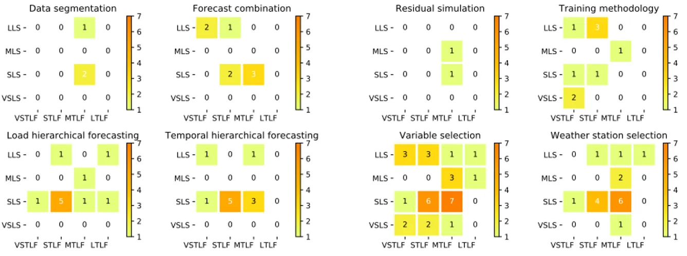
4.2. Forecasting methodologies implemented
This subsection provide the basic principles and references of the forecasting methodologies implemented in the articles reviewed. Figure 6 shows for each forecasting methodology a heat map with the number of implementations by forecasting problem.
VSTLF STLF MTLF LTLF LLS MLS SLS VSLS 0 0 1 0 0 0 0 0 0 0 2 0 0 0 0 0 Data segmentation VSTLF STLF MTLF LTLF LLS MLS SLS VSLS 2 1 0 0 0 0 0 0 0 2 3 0 0 0 0 0 Forecast combination VSTLF STLF MTLF LTLF LLS MLS SLS VSLS 0 1 0 1 0 0 1 0 1 5 1 1 0 0 0 0
Load hierarchical forecasting
VSTLF STLF MTLF LTLF LLS MLS SLS VSLS 1 0 1 0 0 0 0 0 1 5 3 0 0 0 0 0
Temporal hierarchical forecasting 1 2 3 4 5 6 7 1 2 3 4 5 6 7 1 2 3 4 5 6 7 1 2 3 4 5 6 7 VSTLF STLF MTLF LTLF LLS MLS SLS VSLS 0 0 0 0 0 0 1 0 0 0 1 0 0 0 0 0 Residual simulation VSTLF STLF MTLF LTLF LLS MLS SLS VSLS 1 3 0 0 0 0 1 0 1 1 0 0 2 0 0 0 Training methodology VSTLF STLF MTLF LTLF LLS MLS SLS VSLS 3 3 1 1 0 0 3 1 1 6 7 0 2 2 1 0 Variable selection VSTLF STLF MTLF LTLF LLS MLS SLS VSLS 0 1 1 1 0 0 2 0 1 4 6 0 0 0 1 0
Weather station selection 1 2 3 4 5 6 7 1 2 3 4 5 6 7 1 2 3 4 5 6 7 1 2 3 4 5 6 7
Figure 6: Load forecasting methodologies by forecasting problem.
Data Segmentation (DS).
Data segmentation consists in slicing the dataset into several parts and training one or several models on each one or some of them. Then, these models produce forecasts on the corresponding segments where they have been trained. For instance, Chen et al. [31] used only the winter data segment to forecast the January load with support vector regression.
Forecast Combination (FC).
Many authors have suggested the superiority of forecast combinations over the use of individual forecast. Hibon and Evgeniou [69] developed a simple model-selection criterion. The accuracy of the selected combination was significantly better and less variable than the selected individual forecasts.
Forecast combination is similar to the bagging technique. Bagging (bootstrap aggregating) uses bootstrap sam-pling to generate several learning samples, train the model on each one of them and compute the average. Variance is reduced but bias increases a bit because the effective size of a bootstrap sample is about 30 % smaller than the original learning set. However, forecast combination differs from bagging as it consists in combining predictions of different models. There exist several ways of combining forecasts.
Forecast Simple Averaging Combination (FSAC) is the most trivial and consists simply in averaging the fore-casts. Forecast Weighted Combination (FWC) is more refined and consists in using a weighted average. The weights are calculated with different methodologies: manually, by solving an optimization problem, etc. Nowotarski et al. [70] and Nowotarski et al. [71] developed alternative schemes for combining forecasts: simple, trimmed averaging, winsorized averaging, ordinary least squares, least absolute deviation, positive weights averaging, constrained least squares, inverse root mean squared error, Bayesian model averaging, exponentially weighted average, and fixed share machine learning techniques, polynomial weighted average forecasting technique with multiple learning rates, best individual ex-ante model selection in the validation period and best individual ex-ante model selection in the cali-bration window. Ranjan and Gneiting [72] developed a beta-transformed linear opinion pool for the aggregation of probability forecasts from distinct, calibrated or uncalibrated sources.
Residual Simulation (RS).
Residual simulation is a way to produce probabilistic load forecasting by post-processing the point forecasts Hong and Fan [3]. Applying the probability density function of residuals to the point forecasts generates a density forecast. The normality assumption is often used to model the forecasting errors. Xie et al. [33] investigated the consequences of this assumption and showed that it helps to improve the probabilistic forecasts from deficient underlying models but the improvement diminishes as the underlying model is improved. It confirms the importance of sharpening the underlying model before post-processing the residuals. However, if it is not feasible to build comprehensive underlying models, modeling residuals with normal distributions is a plausible method.
Similar day (SD).
The ”similar day” approach considers a ”similar” day in the historic data to the one being forecast. Due to its sim-plicity, it is regularly implemented in industrial applications. The similarity is usually based on calendar and weather patterns. The forecast can be a linear combination or a regression procedure that include several similar days. Taylor [13] implemented a development of this idea in a weather-based forecasting approach which is described by Taylor and Buizza [73].
Temporal Hierarchical forecasting (THF).
Athanasopoulos et al. [74] introduced the concept of temporal hierarchies for time series forecasting, using aggre-gation of non-overlapping observations. By combining optimally the forecasts from all levels of aggreaggre-gation, this methodology leads to reconciled forecasts supporting better decisions across planning horizons, increased forecast accuracy and mitigating modeling risks. Gaillard et al. [27] concatenated a short-term (from one hour to forty-eight hours) and a medium-term (from forty-nine hours to one month) probabilistic forecasting models. Nedellec et al. [20] developed a temporal multi-scale approach by modeling the load with three components: a long, medium, and short-term parts.
Temporal hierarchical forecasting consists also in developing forecasting models for specific time periods. Models for specific hours of the day: one per hour, one per night hours, one for morning hours, one for afternoon, and one for evening hours, etc. Models for specific days: one per week days, one per weekend days, etc. Models for specific time of the year: one per month, one per season, etc.
Training Methodologies (TM).
The way to train a model has a deep impact on the results. Several methodologies exist depending on the past data available and the newly data acquired during the forecast process. Static training methodology consists in training once for all the model with all, or a segment, of data available. Then, it produces forecasts without retraining if newly data are acquired. Accumulative training methodology consists in retraining periodically the model by using newly data acquired and the past data. The retraining period depends on the forecasting horizon. Usually, the smaller the forecasting horizon is, the higher the retraining frequency is. Sliding window methodology consists in using a fixed training data window that is shifted periodically using the newly accumulated data. The shifting period depends on the forecasting horizon. Usually, the smaller the forecasting horizon is, the higher the shifting period frequency is.
Variable selection (VS).
Variable selection assesses the features to use and their functional forms. The goal is to find a small, or the small-est, subset of features that maximizes accuracy. This process enables to avoid overfitting and improves the model performance and the interpretability. It also provides faster and more cost-effective models and reduces the overall computation time. Guyon and Elisseeff [75, 76], Saeys et al. [77], and Friedman et al. [38] are useful references about feature selection. Three main approaches exist for variable selection.
The first one is the filter technique and consists in selecting the relevant features with methods independent of the supervised learning algorithm implemented. The univariate statistical tests (t-test, chi-square, etc.) are fast and scalable but ignore the feature dependencies. The multivariate approaches (decision trees, etc.) take into account the feature dependencies but are slower than univariate. The cross-validation is a powerful tool but can be computationally expensive.
The second approach is the embedded technique. The search for an optimal subset of features is sometimes already built into the learning algorithm. Decision tree node splitting is a feature selection technique, tree ensemble measures variable importance, the absolute weights in a linear support vector machine model, and a linear model with
Least Absolute Shrinkage and Selection Operator provide a feature selection. The embedded technique is usually computationally efficient, well integrated within the learning algorithm and multivariate. However, it is specific to a given learning algorithm.
The last approach is the wrapper technique. It tries to find a subset of features that maximizes the quality of the model induced by the learning algorithm. The quality of the model is estimated by cross-validation. All subsets cannot be evaluated and heuristics are necessary as the number of subsets of p features is 2p. Several approaches exist. Among them, the forward (or backward) recursive feature elimination consists in adding (removing) the variable that most decreases (less increases) the error over several iterations. The wrapper technique is custom-tailored to the learning algorithm, able to find interactions and to remove redundant variables. However, it is prone to overfitting. Indeed, it is often easy to find a small subset of noisy features that contribute to decreasing the score. In addition, this technique is computationally expensive as a model is built for each subset of variables.
Almost all of the articles reviewed adopt a variable selection approach. Hong et al. [8] developed a methodology to select the relevant features for linear regression, fuzzy interaction regression and artificial neural network techniques. The increasing number of relevant features improved the forecast accuracy. Hong et al. [36] extended the method to long-term load forecasting by adding a macroeconomic indicator. As in Hong et al. [8], Charlton and Singleton [18] did a series of refinements to the linear regression benchmark proposed during the Global Energy Forecasting Competition 2012: day-of-season terms, a special treatment of public holidays, and changing the number of seasons. The competition scores were used to demonstrate that each successive refinement step increases the model accuracy.
Weather station selection (WSS).
The weather is a major factor driving the electricity demand, price, wind or solar power generation. Pang [78] details two methodologies to capture the weather impact. The Virtual Weather Station methodology (VWS) consists in a combination (simple average, weighted average, etc.) of the parameters (temperature, wind speed, solar irradiation, etc.) of several weather stations. At the end of the process, the temperature (or solar irradiation, wind speed, etc.) combination can be seen as a parameter from a virtual weather station and is used as a feature for the forecasting models. The Multiple Weather Station (MWS) consists in selecting the weather stations, whose parameters, improve the most the model accuracy. Each one of them is used as feature to feed a forecasting model. The final forecast is the combination (simple average, weighted average, etc.) of the forecasts generated by each model. Based on this principle, Hong et al. [79] developed a framework to determine how many and which weather station selecting for a territory of interest.
5. Use case example and guidelines
Sections 3 and 4 present general guidelines for selecting which forecasting technique or methodology to use in which case. However, the classification process in two dimensions does not take into account the shape or frequency of the load, the quality or length of the data, at which frequency the data are available, etc. Each forecasting problem is thus specific and requires a dedicated customized forecasting model. This section proposes some guidelines, and emphasizes some difficulties that may be encountered to build a first model. It is exemplified on the methodology used in Dumas et al. [80]. The text in italic refers to this case.
5.1. Guidelines
1. Understand and formulate the forecasting problem. What is the application? What are the goals? What is the system considered? Forecasting the consumption and PV production of a microgrid to provide reliable inputs
5. What are the data available? At which frequency is the database updated? What is the quality of the data? The PV and consumption are monitored on site each five seconds. Weather forecasts are available every six hours for the next ten days with a fifteen minutes resolution. Missing data occur rarely.
6. Is data cleansing needed? Missing data are replaced by zero. However, it occurs rarely.
7. What segment of data is considered for the study? Two months of monitored consumption, production, and weather forecasts.
8. Is a benchmark model defined? A linear regression model could have been implemented as benchmark. How-ever, this study focuses on neural networks and gradient boosting regression.
9. What are the forecasting techniques selected? A gradient boosting regression model, a feed-forward and a recurrent neural networks.
10. Is load hierarchical forecasting relevant? No, the microgrid is only composed of one load and the PV monitored is the total production.
11. Is temporal hierarchical forecasting relevant? The forecasts are composed each quarter of ninety-six values as the horizon is twenty-four hours and the resolution fifteen minutes. Thus, it may be interesting to decompose the horizon in two or four parts with a dedicated model for each one. Then, the final forecast could be a combination of each term. However, for the sake of simplicity, the temporal hierarchical forecasting methodology is not implemented.
12. Is forecast combination relevant? It may be interesting to combine neural networks and gradient boosting models. However, for the sake of simplicity, each model is considered independently.
13. What training methodology to use? A sliding window methodology. The learning set has a size of one week and the model is retrained each day.
14. Is weather station selection relevant? No, the models take as inputs the weather forecasts computed at a location close to the microgrid (less than two km).
15. What are the relevant variables of this forecasting problem? Several sets of variables have been tested. The final set is composed of lags of load and temperature weather forecast for the prediction of the consumption. 16. What are the relevant hyper parameters of the models? Several sets of hyper parameters have been tested.
5.2. Forecasting techniques
In some cases, one or several of these general forecasting techniques guidelines may be of good use:
1. Define a benchmark model with a transparent, simple and familiar forecasting technique. Linear regression is recommended for this purpose, see Hong et al. [8, 79], Wang et al. [11], Charlton and Singleton [18], Xie et al. [25, 26], Hong et al. [36]. It is easy to implement, transparent and fast to compute in comparison with more complex techniques such as artificial neural networks, Gaussian process or gradient boosting regression. In addition, customized linear regression models may provide interesting results from very short-term to long-term forecasting. Charlton and Singleton [18] won the load track of the Global Energy Forecasting Competition 2012 with a customized linear regression model.
2. Define a robust methodology to find out the relevant hyper parameters of a given forecasting technique. A blocked form of k-fold cross-validation procedure Bergmeir and Ben´ıtez [81] is recommended when the dataset has a minimum length.
3. Statistical models such as ARIMA or exponential smoothing may provide satisfactory results for horizons of a few hours, where the weather has not a significant impact Taylor [13]. When the horizon is extending to a few days it is recommended to assess the importance of exogenous parameters such as the temperature.
4. Gaussian process provides directly probabilistic forecasts. However, the selection of the relevant kernels is not straightforward and the time computation may be an issue depending on the forecasting problem. In addition, forecasting directly multiple outputs is non-trivial and still a field of active research [82] and [83]. van der Meer et al. [9] used a moving training window to reduce the learning set size and consequently the computational burden of the Gaussian process.
5. Probabilistic forecasting models that produce constant prediction intervals over time provide not useful infor-mation for decision making. Indeed, they do not differentiate periods of high and low uncertainty.
6. Residual simulation based on normality assumption provides a way to generate probabilistic forecasts Xie and Hong [29], Xie et al. [33]. However, this assumption must be assessed. Xie et al. [33] demonstrated that the improvement provided by residual simulation based on the normality assumption is diminishing with the improvement of the underlying model.
5.3. Forecasting methodologies
In some cases, one or several of these general forecasting methodologies guidelines may be of good use.
1. Use a blocked form of cross-validation for time series evaluation Bergmeir and Ben´ıtez [81], van der Meer et al. [9] instead of a traditional k-fold cross-validation. Indeed, the consumption of a utility is a process that might evolves over time, thus hurting the fundamental assumptions of cross-validation that the data are independent and identically distributed.
2. Random forest, Gradient boosting regression, and LASSO are techniques that perform feature extraction. Hong et al. [8] developed a methodology to select the relevant features for linear regression, fuzzy interaction regres-sion and artificial neural network techniques. It can be extended to other techniques.
3. The sliding window training methodology is a way to speed up the time computation by reducing the learning set size van der Meer et al. [9]. However, the accuracy may decrease accordingly. A trade-off should be reached between time computation and accuracy.
4. In some cases, temporal hierarchical forecasting does not improve the results Wang et al. [11], Hong et al. [8]. At the opposite the case studies of Charlton and Singleton [18], Nedellec et al. [20], Taieb and Hyndman [21], Goude et al. [17], Gaillard et al. [27], Haben and Giasemidis [30] benefited from this methodology. The higher the horizon is and consequently the number of points to forecast, the more it is interesting to consider this methodology.
5. The same observation can be done with load hierarchical forecasting. Hong et al. [6] built a case study (D1) to experiment this methodology. Large systems such as distribution networks that are composed of hundreds or thousands of substations such as the case study of Goude et al. [17] may benefit from this methodology to take into account specific locational effects.
6. The weather station selection framework of Hong et al. [79] is recommended when dealing with several possi-bilities for one location.
7. In general, a combination of models improves the results such as in Taylor [13], Lloyd [19], L´opez et al. [24], Xie et al. [26], Xie and Hong [29], Haben and Giasemidis [30].
8. Transforming the data by taking the logarithm before applying Gaussian process may improve the results when considering residential consumption as it is better represented by the log-normal distribution Munkhammar et al. [53], Shepero et al. [15].
9. Probabilistic load forecasting is a specific topic. The Global Energy Forecasting Competition 2014 load track Hong et al. [7] provides a case study (D6) to experiment techniques and methodologies to addressed this prob-lem. Xie and Hong [29] propose an integrated solution composed of pre-processing, forecasting and post-processing to compute probabilistic forecast based on several forecasting techniques.
10. Temperature is often used as input of load forecasting model. However, a temperature forecast with small accuracy may decrease the model performance Chen et al. [31].
6. Conclusion