T
HESE DE DOCTORAT DE
L'UNIVERSITE
DE
NANTES
COMUE UNIVERSITE BRETAGNE LOIRE
ECOLE DOCTORALE N°601
Mathématiques et Sciences et Technologies de l'Information et de la Communication
Spécialité : Informatique, section CNU 27
Probabilistic relational models learning from graph databases
Thèse présentée et soutenue à Nantes, le 02/10/2018
Unité de recherche : Laboratoire des Sciences du Numérique de Nantes (LS2N)
Laboratoire de recherche opérationnelle, de décision et de contrôle de processus (LARODEC)
Thèse N° :
Par
Marwa El Abri
Rapporteurs avant soutenance :
M. Simon De Givry Chargé de Recherche INRA Toulouse M. Nicolas Lachiche Maître de Conférences HDR Université de Strasbourg Strasbourg
Composition du Jury :
Président :
Mme Nahla Ben Amor Professeur des Universités Université de Tunis Tunisie
Examinateurs :
M.Emmanuel Mazer Directeur de Recherche CNRS France
Dir. de thèse :
M. Philippe Leray Professeur des Universités Université de Nantes France
Co-dir. de thèse :
Mme Nadia Essoussi Professeur des Universités Université de Tunis Tunisie
Acknowledgements
This thesis would not have been possible without the inspiration and continuous support of a number of people.
First, I thank the jury’s members who honored me by judging my dissertation. I am grateful for the time they spent to do this.
Then, I want to express my deep gratitude and sincere appreciation to my two supervisors: Pr. Nadia Essoussi who often gave me the courage to move forward in my research, I am thankful for her continuous support, her precious advice and her invaluable help, Pr. Philippe Leray for the constructive discussions, continuous guidance, suggestions, and optimism. I was fortunate to benefit from his expertise in this inter-esting research area. Without them this dissertation would never have been achieved.
I would like to offer my heartiest thanks to my mum for her understanding, support and confidence to which I am forever indebted. Mum, I love you, you have always supported my dreams! To my father’s soul. Dad, may god bless you, I wish you were here to share with us these moments of joy and success.
An honorable mention goes to my family and all my friends especially Montassar and Saif for their help, their company, their emotional support and for listening to my complaints and frustrations. I really love them and I am sure that having brought this work forward is the best reward for them.
More than anything else, I am deeply grateful to my brother Marwen and my sister Maram for their love and continuous moral support.
I would like to express my sincere gratitude to my colleagues either in LARODEC or in DUKe team, especially Rajani Chulyadyo and Thomas Vincent for always sharing their expertise and experiences, and making the development of PILGRIM fun. Their domain expertise has helped me get good insights of PILGRIM.
I would also like to thank all those who have been helped me directly or indirectly in all stages of this thesis.
Contents
I
Introduction and motivations
1
1 Context and issue 3
1.1 Introduction . . . 4
1.1.1 Context . . . 4
1.1.2 Motivation and problem statement . . . 5
1.2 Dissertation organization . . . 7
II
State of the art
9
2 Probabilistic Graphical Models 11 2.1 Introduction . . . 122.2 Basic concepts . . . 12
2.2.1 Concepts related to graph theory . . . 12
2.2.2 Concepts related to probability theory . . . 13
2.3 Bayesian Networks . . . 15
2.3.1 Bayesian Networks formalism . . . 15
2.3.2 Parameter learning . . . 18
2.3.3 Structure learning . . . 20
2.4 Markov Networks . . . 23
2.4.1 Markov Networks formalism . . . 23
2.4.2 Parameter learning . . . 25
2.4.3 Structure learning . . . 26
2.5 Inference in PGMs . . . 27
2.6 Bayesian Networks vs Markov Networks . . . 28
2.7 Conclusion . . . 29
3 Probabilistic Relational Models 31 3.1 Introduction . . . 32
3.2 Basic concepts . . . 32
3.2.1 Entity-Relationship model . . . 33
3.2.2 First-Order-Logic . . . 35
3.3 Direct Acyclic Probabilistic Entity Relationship models . . . 36
3.3.1 DAPERs formalism. . . 36
3.3.2 Extensions: DAPERs with structural uncertainty . . . 39
3.3.3 Parameter learning . . . 39
3.3.4 Structure learning . . . 39
3.4 Markov Logic Networks . . . 40
3.4.1 MLN formalism . . . 40
3.4.2 Parameters learning . . . 43 i
3.4.3 Structure learning . . . 44
3.5 Computing sufficient statistics for PRMs learning . . . 46
3.5.1 Definitions . . . 46
3.5.2 SQL implementation for computing contingency table . . . 47
3.6 Inference in PRMs . . . 48 3.7 Conclusion . . . 48 4 Graph database 51 4.1 Introduction . . . 52 4.2 NoSQL databases . . . 52 4.2.1 CAP theorem . . . 54 4.2.2 BASE properties . . . 54
4.3 Basic concepts related to graph database . . . 55
4.4 Graph database manipulation . . . 57
4.4.1 Subgraph matching . . . 57
4.5 Graph database properties. . . 59
4.6 Graph database use cases . . . 61
4.7 Comparison with other database models . . . 61
4.8 Discussion. . . 62
4.9 Conclusion . . . 63
III
Contributions
65
5 DAPER learning from Graph database using PRM framework 67 5.1 Introduction . . . 685.2 DAPER learning from graph database . . . 68
5.2.1 Principle . . . 69
5.2.2 ER model identification . . . 70
5.2.3 Probabilistic dependencies identification. . . 72
5.3 Experiments . . . 75
5.3.1 Experiment methodology . . . 76
5.3.2 Networks and Datasets . . . 79
5.3.3 Algorithms . . . 80
5.3.4 Evaluation metrics . . . 80
5.3.5 Results and interpretations . . . 82
5.4 Conclusion . . . 89
6 DAPER learning from Graph Database using MLN framework 91 6.1 Introduction . . . 92
6.2 Expressing a DAPER in Markov Logic . . . 92
6.3 DAPER joint learning using MLN framework . . . 95
6.3.1 DAPER joint learning . . . 95
6.3.2 Evaluation process . . . 97
6.4 Experiments . . . 97
6.4.1 Experiment methodology . . . 97
6.4.2 Evaluation metrics . . . 99
6.4.3 Results and interpretations . . . 99
CONTENTS iii 7 Conclusion 107 7.1 Summary . . . 108 7.2 Future works . . . 109
IV
Appendices
111
A PILGRIM relational 113 A.1 Introduction . . . 113A.2 Pilgrim project . . . 113
A.3 PILGRIM Relational . . . 114
A.3.1 Existing libraries . . . 115
A.3.2 Additional libraries . . . 115
A.3.3 Data accessibility . . . 115
A.3.4 PRM specification in PILGRIM . . . 116
A.3.5 Relational schema in PILGRIM . . . 116
A.3.6 PRM learning module . . . 116
A.3.7 PRM benchmark generation module . . . 116
A.3.8 PRM extension module . . . 117
A.3.9 Learning from graph database . . . 118
A.4 Conclusion . . . 121
B Neo4j graph database 123 B.1 Introduction . . . 123
B.2 Neo4j graph database . . . 123
B.2.1 Connecting to Neo4J graph database . . . 124
B.2.2 Cypher query language . . . 126
B.2.3 From relational database to graph database . . . 127
List of Tables
2.1 Example of CPD P (X|Y ) . . . 14
2.2 Example of JPD P (X, Y ) . . . 15
3.1 Example of a first-order knowledge base. Fr() is short for Friends(), Sm() for Smokes(), and Ca() for Cancer() . . . 36
4.1 ACID vs. BASE (Brewer, 2000) . . . 55
4.2 A Comparison of the NoSQL and relational databases . . . 62
5.1 Characteristics of DAPER networks used for naive datasets generation. Values in paren-thesis are min/max values per class. Values in the last column correspond to the maximum length of slot chain kmax and the number of dependencies for each slot chain length (from 0 to kmax). . . 79
5.2 Characteristics of DAPER networks used for respectively naive and k-partite datasets gen-eration. . . 80
5.3 Average ± standard deviation of reconstruction metrics (Precision, Recall, F-score, s-Precision, s-Recall and s-F-score ) when executing RGS with kmax=1 for databases generated from
DAPER1 (top) and DAPER2 (bottom). . . 82
5.4 Average ± standard deviation of reconstruction metrics (Precision, Recall, F-score, s-Precision, s-Recall and s-F-score) for each sample size when executing RGS with kmax = 1 (top) and
kmax=4 (bottom) for databases generated from DAPER3. . . 83
5.5 Average ± standard deviation of reconstruction metrics for each sample size when execut-ing RGS with kmax = 1 (top) and kmax=4 (bottom) for databases generated from DAPER’3. 84
5.6 Average ± standard deviation of reconstruction metrics for each sample size when execut-ing RGS with kmax = 1 (top) and kmax=4 (bottom) for databases generated from DAPER"3. 85
5.7 Average ± standard deviation of reconstruction metrics for DAPER3 for a particular size (3000 instances) with a percentage α of exceptions in the relationship instances for λ fixed to 10% . . . 86
5.8 Average ± standard deviation of reconstruction metrics for DAPER3 for a particular size (3000 instances) with a percentage λ of ER identification for α fixed to 50%. . . 86
5.9 A table of running time (in seconds) for each sample size, when executing RGS_Neo4j with naive datasets and k-partite datasets generated from each DAPER. . . 87
6.1 Knowledge base corresponding to the DAPER described in Figure 6.1. . . 93
6.2 characteristics of DAPER networks used for dataset generation. Values in parenthesis are min/max values per class. Values in parenthesis are min/max values per class. Values in the last column correspond to the maximum length of slot chain kmax and the number of dependencies for each slot chain length (from 0 to kmax). . . 98
6.3 Average ± standard deviation of RSHD_ER for DAPERs for a particular size (5000 instances).101 v
6.4 Average ± standard deviation of RSHD_PD for each algorithm for a particular sample size and network with a percentage α of exceptions in the relationship instances fixed to 10% . Bold values present the best values for a given model and a given sample size. . . 102
6.5 Average ± standard deviation of RSHD_PD for each algorithm for a particular sample size and network with a percentage α of exceptions in the relationship instances fixed to 30% . Bold values present the best values for a given model and a given sample size. . . 103
6.6 Average ± standard deviation of RSHD_PD for each algorithm for a particular sample size and network with a percentage α of exceptions in the relationship instances fixed to 50% . Bold values present the best values for a given model and a given sample size. . . 104
6.7 A comparative study of obtained optimum values of both methods using the statistical stu-dent test with a critical threshold= 5%. . . 106
List of Figures
1.1 Thesis synopsis. . . 7
2.1 Example of graphical models . . . 13
2.2 Example of Bayesian Network. . . 16
2.3 The rules of Bayes Ball theorem . . . 17
2.4 Markov equivalence. . . 18
2.5 Example of Markov Network . . . 24
2.6 (a) A DAG; The dotted red node X8 is independent of all other nodes (black) given its Markov blanket, which includes its parents (blue), children (green) and co-parents (orange). (b) The same model represented as a MN; The red node X8is independent of the other black nodes given its neighbors (blue nodes) (Koller and Friedman, 2009). . . 28
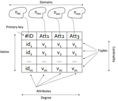
3.1 An example of (a)ER diagram, (b) instance I and (c)skeleton σERfor the university domain. 34 3.2 Relation components . . . 34
3.3 An example of DAPER model which corresponds to the ER model and Instance given in Figure 3.1. Slot chains are not represented in order to simplify the figure. . . 38
3.4 An example of MLN for the university domain. The pairs of formulas and weights together with the set of constants construct the ground Markov network. . . 42
3.5 Excerpt from the CT table for the attribute student.ranking and its parent as they are linked in the DAPER of Figure 3.3. . . 47
4.1 Example of Key-Value store. . . 53
4.2 Example of Column Family database. . . 53
4.3 Example of Document database. . . 54
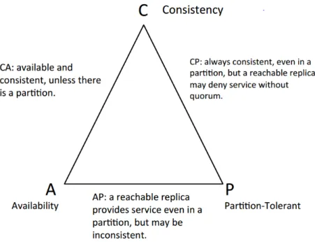
4.4 The CAP theorem (Brewer, 2000) . . . 55
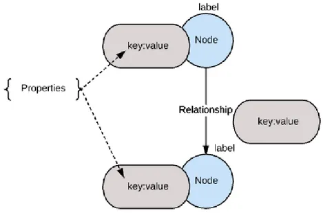
4.5 The graph database components. . . 57
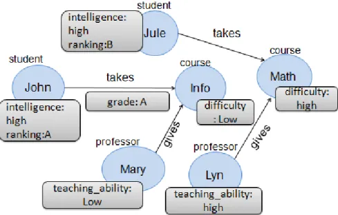
4.6 Example of graph database for the university domain. . . 58
4.7 Example of graph database . . . 59
4.8 Example of subgraph matching. . . 59
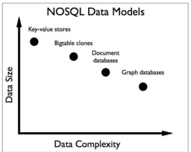
4.9 Categorization of NOSQL databases. . . 62
5.1 Step I: ER schema identification from a graph database. . . 69
5.2 Step II: Computation of sufficient statistics and DAPER learning using the ER schema already identified and the graph database instance. . . 69
5.3 Pattern element. . . 73
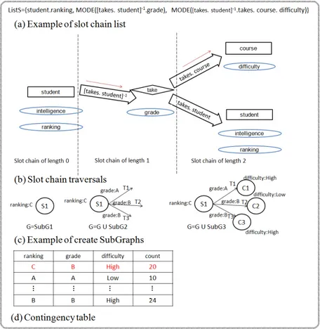
5.4 Illustration of counting sufficient statistics process for the attribute student.ranking and its parents. . . 74
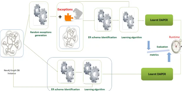
5.5 Evaluation process of a DAPER structure learning from usual relational database versus graph database. . . 76
5.6 Evaluation process of a DAPER structure learning from "noisy" graph database . . . 78 vii
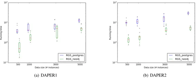
5.7 Boxplot of running time (in seconds and log scale) for each sample size, when executing RGS_postgres and RGS_neo4j with kmax=1 and databases generated from DAPER1 (a) and
DAPER2 (b). . . 83
5.8 Boxplot of running time (in seconds and log scale) for each sample size, when executing RGS with kmax=1 (a) and kmax=4 (b) and databases generated from DAPER3. . . 84
5.9 Boxplot of running time (in seconds and log scale) for each sample size, when executing RGS with kmax=1 (a) and kmax=4 (b) and databases generated from DAPER’3. . . 85
5.10 Boxplot of running time (in seconds and log scale) for each sample size, when executing RGS with kmax=1 (a) and kmax=4 (b) and databases generated from DAPER"3. . . 86
5.11 An example of screenshot of the structure of strongly connected (naive) and dispersed k-partite) graph databases. . . 88
5.12 An illustration of normal and critical paths. . . 89
6.1 Example of a DAPER model (inspired from (Getoor, 2001) and detailed in Chapter 3). . . 93
6.2 Process of DAPER joint learning using MLN framework. . . 96
6.3 The Average values of RSHD_ER with respect to λer when executing approach 1 and 2 with (a) α=30% and (b) α=50% for a particular size (5000 instances) of DAPER1. . . 100
6.4 The Average values of RSHD_PD with respect to λpd when executing approach 1 and 2 with (a) Data size =1000 and (b) Data size =3000 and (c) Data size =5000 for DAPER1 with a percentage α of exceptions in the relationship instances fixed to 10%. . . 101
6.5 The Average values of RSHD_PD with respect to λpd when executing approach 1 and 2 with (a) Data size =1000 and (b) Data size =3000 and (c) Data size =5000 for DAPER1 with a percentage α of exceptions in the relationship instances fixed to 30%. . . 102
6.6 The Average values of RSHD_PD with respect to λpd when executing approach 1 and 2 with (a) Data size =1000 and (b) Data size =3000 and (c) Data size =5000 for DAPER2 with a percentage α of exceptions in the relationship instances fixed to 30%. . . 103
6.7 The Average values of RSHD_PD with respect to λpd when executing approach 1 and 2 with (a) Data size =1000 and (b) Data size =3000 and (c) Data size =5000 for DAPER2 with a percentage α of exceptions in the relationship instances fixed to 50%. . . 104
6.8 Boxplot of running time (in seconds and log scale) for each sample size of each DAPER. . 105
7.1 A new definition for DAPER model in context of graph databases. . . 109
A.1 Class diagram for the RelationalSchema, Class, Attribute and Domain classes. . . 117
A.2 Implementation environment . . . 118
A.3 Class diagram for Neo4jGenerator and Neo4jRequest.. . . 119
A.4 Class diagram for Neo4jInstance . . . 120
B.1 Neo4j graph database model. . . 124
B.2 Neo4j graph database features. . . 125
B.3 The Neo4j browser. . . 125
B.4 A HTTP request example which executes Cypher query to create a Person.. . . 126
B.5 A "Hello world" example shows the minimal configuration necessary to interact with Neo4j through a driver designed for C language. . . 127
B.6 A social graph describing the relationship between three friends. . . 128
B.7 A Cypher pattern example. . . 128
B.8 A Cypher query example contains MATCH and RETURN clauses. . . 128
B.9 Cypher versus SQL language. . . 129
B.10 The three most common paradigms for deploying relational and graph databases (Hunger et al., 2016). . . 129
List of Algorithms
1 Relational Greedy Search (Friedman et al., 1999a) . . . 40
2 Generate_Neighbors . . . 41
3 MLN structure learning (Kok and Domingos, 2005) . . . 45
4 Find_Best_Clause (Kok and Domingos, 2005) . . . 45
5 ER_Model_identification . . . 70 6 Get_Filtered_Relationship_Classes . . . 72 7 Get_Counts . . . 76 8 Create_Slot_chain_Traversals . . . 76 9 Create_SubGraphs . . . 77 ix
I
Introduction and motivations
1
Context and issue
Contents
1.1 Introduction . . . 4
1.1.1 Context . . . 4
1.1.2 Motivation and problem statement . . . 5
1.2 Dissertation organization . . . 7
1.1
Introduction
1.1.1
Context
Machine Learning (Bishop, 2006) is a field of artificial intelligence aimed at defining efficient methods for data mining and knowledge extraction. This knowledge is generally represented in the form of functions, mathematical or statistical models. Learning is divided into deductive learning and inductive one. The first one consists of starting from generalizations (rules) to specific examples. Inductive learning consists of learning from examples, to induce patterns or hypotheses from the given input data for predicting new data (predictive modeling) or for describing the input data (descriptive modeling).
Historically, the vast majority of techniques in Machine Learning has focused on flat data also called propositional data or attribute-value representation. Flat data is a single-table or single-tuple format where each row represents a data instance, and each column represents an attribute.
A critical assumption made by these techniques on flat datasets is that their individuals are Independently and Identically Distributed (IID). These algorithms admit that the data instances are drawn independently from each other from a same distribution. Examples of such dataset are available on UCI Machine Learning repository1 include well known Iris dataset2 , Wine dataset3 etc., which have been used in many research
studies.
Many real cases involve unsure data. In fact, we are often uncertain about the real state of the data because our observations about it are partial (only some aspects of the world are observed)or noisy (even those aspects that are observed are often observed with some errors). The real state of the world is rarely determined with certainty because of our limited observations as if relationships are not deterministic. For example, there are few diseases where we have a clear and deterministic relationship between the disease and its symptoms. These domains can be characterized regarding to a set of random variables, where the value of each variable defines an essential property of the world.
In the early stage of research in Machine Learning, many techniques were proposed in many research communities. Not all techniques can support real-world uncertainty, contrariwise the framework of Proba-bilistic Graphical Models(PGM) (Koller and Friedman, 2009). There are two major types of PGMs, directed graphical models such as Bayesian Network (BN) (Pearl, 1988), and undirected graphical models such as Markov random fields (MRFs) or Markov Networks (MN) (Pearl, 1988). PGMs become quickly an impor-tant tool to address real-world applications where uncertainty is almost an inescapable aspect. They allow to reason probabilistically about the values of one or set of variables, given observations about some others by efficiently encoding a joint distribution over the space of possible assignments of random variables. They are designed to work with flat data using a graph-based representation.
However, many real-world data sets are innately relational. Such data consist of entities of different types, where a different set of attributes characterizes each entity type. Entities are related to each other via various kinds of links, and the link structure is an essential source of information.
Relational data can be represented as a multi-table format where each table corresponds to an entity type or a relationship type. Each row in an entity table represents an entity/object, and each row in a relationship table denotes the relationship between objects.
As objects are related to each other, the IID hypothesis of individuals in tabular data set is often unre-alistic. Indeed, according to this hypothesis, no individual can influence other people. Or, individuals are generally not merely data records, but interact with each other, generating many links between them. The IID hypothesis contradicts the so-called autocorrelation phenomena often observed in the real world. For instance, the fact that the cultural tastes of a person depend on those shared by his friends. The knowledge obtained on an individual can then give information about the others, and the individuals can not, therefore, be considered as IID. Thus, the IID assumption is often violated in relational data contexts. This limits the
1. https://archive.ics.uci.edu/ml/index.php 2. https://archive.ics.uci.edu/ml/datasets/Iris 3. https://archive.ics.uci.edu/ml/datasets/Wine
1.1 Introduction 5 application of PGMs on relational data. Consequently, Statistical Relational Learning (SRL) (Taskar et al., 2007;Neville and Jensen, 2005) has emerged as a branch of machine learning that is concerned with sta-tistical analysis on domains with complex relations and uncertainty. The presence of multiple interrelated aspects characterizes complex systems. Or, many real cases involve both complex and uncertain relational data.
During the last decade, various approaches have been proposed to deal with relational and statisti-cal learning. Probabilistic Relational Models (PRMs) are one of the most used models to handle uncer-tainty in a relational context. PRMs present a relational extension of PGMs, such as Relational Bayesian Networks (RBN) (Koller and Pfeffer, 1998;Friedman et al., 1999a), Directed Acyclic Probabilistic Entity-Relationships models (DAPER) (Heckerman and Meek, 2004) and Markov Logic Networks (MLN) ( Richard-son and Domingos, 2006).
PRMs have shown the importance of relaxing the IID assumption. They can handle well structured relational data stored in relational databases for which a relational schema is defined in advance.
In the following section, we will describe the motivating scenario for this thesis and state the problems we try to address.
1.1.2
Motivation and problem statement
With the rise of the Internet, numerous technological innovations and web applications are driving the dramatic increase in data. For example, Facebook, Twitter, and other forms of social media sites, location-based services, smartphones, and other consumer mobile devices including PCs, mobile phones, laptops have allowed billions of individuals around the world to contribute to the amount of the available data. Much of that data does not come only from the web and social networks, but also, from sensor networks. Indeed, technological devices are made up of enabled embedded devices connected to the Internet, including sensors, active positioning tags, and radio-frequency identification (RFID) readers. For example, today some roads have sensors and can communicate with the vehicles passing over them to determine traffic patterns and find more sustainable ways to route cars. Also, texts, pictures, log files, videos, etc. generate a tremendous amount of unstructured data. Much of them are gathered in real time and provide a unique compelling opportunity if they can be analyzed and acted in real time. All these technologies and new forms of personal communication are driving the extensive collection of unstructured and complex datasets.
Consequently, Big Data has emerged as traditional techniques of process and storage that can not deal with a large amount of various and uncertain data coming in fast streaming.
According to (Sun and Reddy, 2013), Big data consists of the major four V’s namely "Volume" which means simply lots of data gathered by a company. "Variety" refers to the type of data that Big Data can comprise, data can be structured as well as unstructured. "Velocity" refers to the speed of data generation and the time in which Data Stream can be processed. "Veracity" deals with the uncertainty of data. Each one of these Vs consists of a whole issue that researchers and developers want to solve. So, the challenge for Big Data is how to deal with these issues.
Today, the most of services and sites such as Facebook, Google, Yahoo, etc. have a billion entries in their databases, as many daily visits. Accordingly, one machine cannot handle the whole database. Besides, for reasons of reliability, these databases are duplicated to do not interrupt a service in case of failure or breakdown. The method consists of adding servers to duplicate data and thus increase performance and resist to breakdown. Therefore, two problems appear. First, the storage cost is enormous because each data is present on each server. Second, the cost of insertion/ modification/ deletion is great, because we can not validate transaction if we are not certain that it was performed on all servers and system makes user waiting during this time. This leads to a difficulty of scaling. Also, certain types of queries are not optimized using a relational database, specially queries that consume a huge number of joins between tables. A join means a Cartesian product, so a request with many joins in an extensive database where data are strongly linked takes a lot of time and even can fail. Relational databases cannot cope with all these requirements. Thus, with the emergence of Big data, the need for more flexible databases is evident.
This problem has been recently addressed by a new brand category of data management systems that do not use SQL exclusively, the so-called NoSQL movement (Partner et al., 2014). NoSQL includes four sig-nificant types of databases: key/value, oriented document, oriented column, and graph databases. Recently there has been an increasing interest in graph databases to model objects and interactions. In contrast to re-lational databases, where join-intensive query performance deteriorates as the dataset gets more prominent, a graph database depends less on a rigid schema, and its performance tends to remain relatively constant, even as the dataset grows. This is can be explained by the fact queries are expressed in terms of graph traversal operations which are localized to a portion of the graph.
Consequently, graph databases are rapidly emerging as an effective and efficient solution to the man-agement of extensive datasets in scenarios where data are firmly connected, and data access mainly rely on traversing theses graphs.
Graph databases are unstructured and schema-free data stores. Edges between nodes can have various signatures. In other words, some edges (relationships) that do not correspond to the ER model could be depicted without any problem in the graph database. These relationships are considered as exceptions.
As we have discussed in the previous section, PRMs can be used for learning and reasoning from re-lational datasets. Using PRMs in Big Data context has been little-tackled topic of research. No work has been identified for PRMs learning from partially structured graph databases.
In this thesis, we are particularly interested in the task of learning PRMs from graph databases. Our focus is on DAPER and MLN models.
This thesis addresses three main issues:
1. How to adapt DAPER learning methods to handle unstructured and various data stored in the graph database?
2. How to deal with "noisy" datasets which contain exceptions?
3. How Markov logic framework can be used for DAPER learning from partially structured graph database?
Consequently, our first contribution is the proposition of an algorithmic approach allowing to learn DAPER model from a graph database.
The originality of this process is that it allows to first identify an Entity Relationship model automati-cally from an existing graph database instance. As in our graph database, a same typed relationship could be used to connect pairs of vertices with different pairs of classes, our identification approach allows to man-age exceptions by considering each relationship label and each corresponding signatures that are enough represented for this label in the database.
Our objective is to learn DAPERs with less structured data and to accelerate the learning process by querying graph databases. This work was presented at AICCSA 2017 and will be explained in detail in Chapter5.
In our second contribution, we are interested by another probabilistic relation model which rely on the possible-world semantics of first-order probabilistic logic namely MLN. Our proposed method consists of DAPER learning from partially structured graph databases using MLN frameworks. MLN can help us to take into account the exceptions that are dropped during DAPER learning. We propose a joint learning from partially structured graph databases, where we want to learn at the same time the ER schema and the probabilistic dependencies. This contribution is introduced in ICDEc 2018 and will be more explained in Chapter6.
Finally, we contribute to the development of PILGRIM (ProbabIListic GRaphIcal Model) software. A tool developed by our research group DUKe. This thesis has made significant contributions in the
imple-1.2 Dissertation organization 7
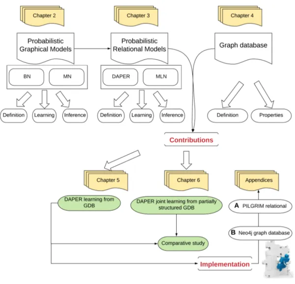
Figure 1.1 – Thesis synopsis.
mentation of a new interface to first be able to communicate with Neo4j4 graph database as well as the
development of functionalities that allow PRM learning from graph database instance.
1.2
Dissertation organization
Figure1.1presents the thesis organization and interdependencies between chapters.
Chapter2is dedicated to introducing Probabilistic Graphical Models, notably Bayesian Networks and Markov Networks and to make a survey on existing learning approaches.
Chapter3 is dedicated to the introduction of extensions of Probabilistic Graphical Models, more pre-cisely Direct Probabilistic Entity Relationship and Markov Logic Network models by giving their definition and their learning methods.
Chapter4gives an overview of graph database principles. Then, we give a formal definition of the graph database and discuss its properties. Finally, we provide a brief comparison between the graph databases and the most used databases.
Chapter5describes our first contribution which is divided into twofold. First, we present how to extract the underlying ER model from a partially structured graph database. Then, we describe a method to com-pute sufficient statistics (counts) based on graph traversal techniques.
Chapter 6 describes our second contribution which consists of DAPER joint learning from partially structured graph databases using an MLN framework, where we want to learn at the same time the ER schema and the probabilistic dependencies. The Markov Logic Network formalism seems an efficient so-lution for this task. Both parts of the models are described in the same logical way, and dedicated structure learning algorithm could be able to retrieve both information at the same time. The logical formulas used to describe the model can also manage exceptions, i.e., data which are not coherent with an underlying structured model, as we have to deal with when working with partially structured data.
Chapter 7 presents our conclusions, and point towards some prospects of future research in the area addressed by this thesis.
AppendicesA andBpresents environments and software used during the development phase and our implementation process.
II
State of the art
2
Probabilistic Graphical Models
Contents
2.1 Introduction . . . 12
2.2 Basic concepts . . . 12
2.2.1 Concepts related to graph theory . . . 12
2.2.2 Concepts related to probability theory . . . 13
2.3 Bayesian Networks. . . 15
2.3.1 Bayesian Networks formalism . . . 15
2.3.2 Parameter learning . . . 18
2.3.3 Structure learning . . . 20
2.4 Markov Networks . . . 23
2.4.1 Markov Networks formalism . . . 23
2.4.2 Parameter learning . . . 25
2.4.3 Structure learning. . . 26
2.5 Inference in PGMs . . . 27
2.6 Bayesian Networks vs Markov Networks . . . 28
2.7 Conclusion . . . 29
2.1
Introduction
In traditional machine learning settings, data is usually expected to consist of a single type of object, and the objects in the data are assumed to be independent and identically distributed (IID).
One of the most known techniques in model-based machine learning from flat data consists in con-structing graphical models which also fits within the dependence analysis framework and corresponds to extracting dependency relations from observed data to make predictions.
Probabilistic Graphical Models (PGM) (Koller and Friedman, 2009) have become a viral tool for dealing with uncertainty through the use of probability theory, and a practical approach to coping with complexity using graph theory. They represent the probability distribution of a set of random variables in combination with dependent variables using graphs.
There are two major types of PGMs, directed graphical models such as Bayesian Network (BN) (Pearl, 1988), and undirected graphical models such as Markov Random Fields (MRFs) or a Markov Networks (MN) (Pearl, 1988).
The two main tasks of PGMs are learning and inference. Learning implies the identification of both components of the model (structure and parameters). Inference task consists of studying the impact of some partially observed variables known as evidence on remaining ones.
Parameter learning of BN and MN consists of identifying a set of conditional probabilistic distribu-tions (CPDs) of the BN or to identify a set of parameters which define the potential funcdistribu-tions of the MN. Structure learning of BN and MN consists of determining the set of probabilistic dependencies between discrete random variables in the network. Several approaches have been proposed to address these tasks. The inference task consists of studying the impact of some partially observed variables known as evidence on remaining ones given a specific fixed joint probability distribution, in which case the difference between BN and MN are less important. Indeed, same inference methods can be applied to BN and MN.
The remainder of this chapter is as follows: Section 2.2 recalls some basic concepts from graph and probability theories. A detailed description and definition of these two models with their graphical rep-resentation are presented in Sections 2.3 and 2.4. Sections 2.3.2 and 2.4.2 introduce parameter learning methods for BN and MN respectively. Sections2.3.3and2.4.3present BNs and MLNs structure learning approaches. Section 2.5 goes through inference task in both models. A brief comparison between both models is given in Section2.6.
2.2
Basic concepts
Bayesian Network and Markov Network are founded on both graph and probability theories. Thus, it is useful to recall some valuable concepts from these theories before addressing these models. All these concepts and definitions are derived (Diestel, 2005) and (Durrett, 2009;Renyi, 2007).
2.2.1
Concepts related to graph theory
Definition 2.2.1. Graph
A graphG = (V, E) is a finite collection of nodes (or vertices) V = {n1, n2, ..., nN} and set of edges (or links)E ⊂ {(u, v) k u, v ∈ V }
Definition 2.2.2. Neighbor
2.2 Basic concepts 13 Definition 2.2.3. Directed graph
A directed graph is a graph in which all edges are directed is a directed graph. Definition 2.2.4. Undirected graph
An undirected graph is a graph in which all edges are undirected is an undirected graph. Definition 2.2.5. Moral graph
A moral graph of a directed acyclic graph G is formed by adding edges between all pairs of nodes that have a common child and then making all edges in the graph undirected.
Definition 2.2.6. Complete graph
A complete graph is a graph in which an edge connects every pair of nodes is a complete graph. Definition 2.2.7. Clique
A clique is a complete subgraph of a graph G. Definition 2.2.8. Maximal clique
Clique with a maximal number of nodes; cannot add any other node while still retaining complete connect-edness.
Definition 2.2.9. Path
A path in a graph is a finite or infinite sequence of edges which connect a sequence of vertices. Definition 2.2.10. Directed path
A directed path is a path in which all edges are directed in the same direction is a directed path. Definition 2.2.11. Directed cycle
A directed cycle is a directed path starting and ending at the same vertex. Definition 2.2.12. Directed Acyclic Graph(DAG)
A Directed Acyclic Graph is a graph that contains only directed edges and no cycles is called a directed acyclic graph (DAG). Given a graph G with four nodesX1,X2,X3, andX4,
if there is a directed edge fromX1toX2, thenX1 is a parent ofX2, andX2 will be the child ofX1. If there is a directed path fromX1toX4, thenX1 is an ancestor ofX2 andX2is a descendant ofX1.
(a) A complete graph (b) A directed acyclic graph
(c) An undirected
graph Figure 2.1 – Example of graphical models
2.2.2
Concepts related to probability theory
Definition 2.2.13. Random variable
A random variable is a variable whose possible values are numerical outcomes of a random phenomenon. There are two types of random variables, discrete and continuous.
Y0 Y1 X0 0.2 0.8 X0 0.8 0.2
Table 2.1 – Example of CPD P (X|Y )
Definition 2.2.14. Domain of values
The Domain of values is the number of states (values) associated with random variable known as the domain of values. The finite domain of the variable X is denoted byD(X) .
Let us denote by lower case letters (x, y, z, ...) the value taken by the corresponding variable (X, Y, Z, ...). Definition 2.2.15. Probability distribution
The probability distribution P (X) of a discrete random variable X is a list of probabilities P (X = x) associated with each of its possible valuesx ∈ D(X).
The probability of an eventx ∈ D(X) is non-negative, P (X = x) > 0 and the probabilities of all events sum to one,
Σxi∈D(X)P (X = xi) = 1
Definition 2.2.16. Conditional Probability Distribution CPD
Given two random variables X, Y, the distribution over X conditioned on Y denotedP (X, Y ) defines a dis-tribution over X for each possible value of Y. (e.g., Table2.1is an example of CPDP (X|Y ).
Generally, the conditional probability of X = x under the condition Y = y (evidence) is defined as:
P (x|y) = P (x, y)
P (y) (2.1)
Definition 2.2.17. Bayes theorem
P (X|Y ) = P (Y |X)P (X)
P (Y ) (2.2)
Definition 2.2.18. Conditional independence
Let three random variables X, Y and Z. X and Y are conditionally independent to Z(notedX ⊥ Y |Z) if and only if:
P (X|Y, Z) = P (X|Z) or
2.3 Bayesian Networks 15 X0Y0 X0Y1 X1Y0 X1Y1
0.3 0.5 0.1 0.1
Table 2.2 – Example of JPD P (X, Y )
Definition 2.2.19. Joint Probability Distribution (JPD)
For a set of random variablesXi, i = 1, 2, ..., n, the joint probability distribution is defined to be the dis-tribution over all variablesP (X1, ..., Xn). To determine the joint distribution of n random variables, the cartesian product of all the random variables domains must be provided. If each variable has k states, then there arekn combinations. This product is exponential on the number of variables. (e.g., the Table 2.2is an example of joint distributionP (X, Y ) for two binary variables X, Y.
More generally, a joint distribution over n random variables may be expressed using conditional probabil-ities as follows: P (X1, ..., Xn):DX1 × ... × DXn → [0, 1] (x1, ..., xn) 7→ P (x1, ..., xn) = P ( \ i∈{1,...,n} {Xi = xi}) (2.3)
whereDX is the domain of the random variableX, and corresponding lower-case letter x denotes the assignments or states of X.
2.3
Bayesian Networks
2.3.1
Bayesian Networks formalism
Bayesian Network (BN) (Pearl, 1988) is known as a directed acyclic graph (DAG) in which nodes are random variables, while the edges between the nodes represent probabilistic dependencies among the corresponding random variables. Nodes that are not connected by edges are variables that are conditionally independent of each other. Nodes that are connected by edges do have conditional, dependent relationships. BN enables a representation and computation of the joint probability distribution (JPD) over a set of random variables. This JPD can be determined uniquely by these local conditional probability tables (CPTs). In this section, a formal definition of the Bayesian network (Pearl, 1988) is given. Then, we recall the d-separation criterion. Finally, we present the Markov equivalence class for directed acyclic graphs.
2.3.1.1 Bayesian Network definition
Formally, Bayesian Network B =< G, θ > is defined by:
— A graphical (qualitative) component consists of a directed acyclic graph (DAG) G = (V, E) where V is the set of vertices (nodes) X1, X2, . . . , Xnrepresents random variables. E is the set of directed edges that describes the direct dependencies between these variables.
— A numerical (quantitative) component consists of a set of parameters θ = {θ1, ..., θn} where each θi = {P (Xi|P a(Xi))} represents the set of probabilities for each node Xi conditionally to the states of its parents P a(Xi) in G.
Example 2.3.1. An example of a Bayesian network is shown in Figure2.2 which illustrates four random variables "Difficulty, Intelligence, Grade and Ranking". This network demonstrates the influence between the ranking of student and its grade giving its intelligence and course’ difficulty.
Figure 2.2 – Example of Bayesian Network. 2.3.1.2 Conditional Independence in Bayesian Networks
A BN reflects a simple conditional independence statement called local Markov property.
Property 2.3.1. (Local Markov Property): Each variable is independent of its non descendants N d(Xi) in the graph given its parentsP a(Xi).
Xi ⊥ N d(Xi)|P a(Xi)
Example 2.3.2. In the figure 2.2 Ranking is independent of Dif f iculty, Intelligence given its parent Grade.
The conditional independence relationships encoded by a BNs are devised into three type of connec-tions; serial, diverging and converging connections.
The three types of connections as illustrated in Figure2.3.
— Serial connection: consider the case in which there is one incoming and outgoing arrow to Y , X → Y → Z. It is intuitive that the nodes upstream and downstream of Y are dependent if Y is hidden. — Diverging connection: when there are two diverging arrows from Y, X ← Y → Z. Y is a "root". If
Y is hidden, the children are dependent, because they have a hidden common cause, so the ball passes through. If X is observed, its children are rendered conditionally independent, so the ball does not pass through.
— Converging connection (collider or v-structure): when two arrows are converging on a node X → Y ← Z with Y is a "leaf". If Y is hidden, its parents are marginally independent, and hence the ball does not pass through (the ball being "turned around" is indicated by the curved arrows); but if Y is observed, the parents become dependent, and the ball does pass through.
Given these three type of connections, BN encodes a critical criterion called d-separation. Thanks to this criterion a joint probability distribution encoded by a Bayesian Network can be factorized into a local probability distribution.
Definition 2.3.1. Let G = (V,E) be a DAG and let X, Y, and Z be disjoint sets of variables in V:
— A path from someX ∈ X to some Y ∈ Y is d-connected given Z if and only if every collider W on the path, or a descendant ofW, is a member of Z and there are no non-colliders in Z.
2.3 Bayesian Networks 17
Figure 2.3 – The rules of Bayes Ball theorem
— X and Y are said to be d-separated by Z if and only if there are no d-connecting paths between X and Y given Z.
Example 2.3.3. In Figure2.2, IfGrade is not observed, Dif f iculty and Ranking are dependent. If Grade is observed, Dif f iculty and Ranking are conditionally independent; this path is a serial connection. If Grade is not observed, Dif f iculty and Intelligence are independent; this path is a converging connection having its middle node Grade. If Grade is observed, Dif f iculty and Intelligence are conditionally dependent.
Accordingly, a Bayesian Network B defines a unique join probability distribution over V, namely:
PB(X1, X2, . . . , Xn) = n Y i=1 PB(Xi|P a(Xi)) = n Y i=1 θXi|P a(Xi) (2.4)
This function is decomposed into a product of terms depending only on the local node and its parents in the graph that is a significant result, and very useful of the local Markov Property2.3.1that verifies each variable Xi is independent of its non descendants given its parents in G.
2.3.1.3 Markov equivalence class for Directed Acyclic Graphs
Different DAGs can have the same d-separations. We say that they are Markov equivalent.
Definition 2.3.2. Let {G1 = V, E1} and G2 = {V, E2} be two DAGs containing the same set of nodes V. ThenG1 andG2are called Markov equivalent if for every three mutually disjoint subsetsA, B, C ⊆ V , A, andB are d-separated by C in G1if and only ifA and B are d-separated by C in G2. That is
IG1(A, B | C) ⇔ IG2(A, B | C)
Theorem 2.3.1. Two DAGs are Markov equivalent if and only if, based on the Markov condition, they entail the same conditional independence.
Figure 2.4 – Markov equivalence
Example 2.3.4. Let’s consider the Figure2.4. In this example, it can be easily demonstrated thatG1 and G2are equivalent by the decomposition of their joint probability distributions (Naïm et al., 2011). We have:
P (X1, X2, X3)G1 = P (X2 | X1) ∗ P (X1 | X3) ∗ P (X3) and P (X1, X2, X3)G2 = P (X2 | X1) ∗ P (X3 | X1) ∗ P (X1) Thus P (X1, X2, X3)G2 = P (X2 | X1) ∗ P (X3 | X1) ∗ P (X1) = P (X2 | X1) ∗ P (X1 | X3) ∗ P (X3) P (X1) ∗ P (X1) = P (X2 | X1) ∗ P (X1 | X3) ∗ P (X3) = P (X1, X2, X3)G1
Similarly, it can be demonstrated that G3 is equivalent to G1 and G2. These three networks are not equivalent to the v-structure G4. As P (X1, X2, X3)G4 = P (X1 | X2, X3) ∗ P (X2) ∗ P (X3) and P (X1 |
X2, X3) cannot be simplified.
Markov equivalence is redefined regarding the concepts of skeleton and v-structure by the following theorem, initially introduced by (Verma and Pearl, 1990).
Theorem 2.3.2. Two DAGs are equivalent if and only if they have the same skeletons and the same v-structures.
The main two tasks performed by a Bayesian network are learning and inference. BN learning implies structure learning and parameter estimation from data. Parameter estimation consists of identifying the set of probability distributions using either the statistical approach or the Bayesian one. Structure learning consists of determining the set of probabilistic dependencies of the network. Once the BN is learned, the inference can be performed. In the following sections, we focus on BN parameter and structure learning from complete data.
2.3.2
Parameter learning
The joint probability is given by Equation 2.4 of a domain which can be factorized into smaller and local distribution. Each local distribution involves a node and its parents only. Parameter learning means to estimate these CPDs from data. In the parameter estimation task, we assume that the qualitative dependency structure of the graphical model is known.
2.3 Bayesian Networks 19 Suppose that we have n discrete variables, x1, ..., xn, and n complete observations D = {(x
(l) k1, ..., x
(l) kn), l =
1, ..., n}. Each observation contains a value assignment to all the variables in the model. There are two classes of approaches for learning the CPDs of a given structure. The statistical approach consists of estimating the probability of an event by its frequency of occurrence in the database known as the maximum likelihood estimation. The Bayesian approach consists on finding the most likely parameter knowing that the data were observed using some prior.
2.3.2.1 Statistical approach
The statistical approach consists of estimating the probability of an event by calculating its occurrence frequency in the dataset. The statistical approach based on the Maximum Likelihood (MV) criterion, i.e., the probability of the data given the BN is maximal. Given the complete data D, the MV function is:
ˆ
P (Xi = xk|pa(Xi) = xj) = ˆθi,j,kM V =
Ni,j,k
ΣkNi,j,k
(2.5) where, Nijk is the number of samples in the database for which Xi is on its kth configuration for parent configuration xj.
Despite, this approach has its disadvantageous because when some configurations do not exist in the dataset, the corresponding parameter will be evaluated by a zero value. Thus, the Bayesian approach was introduced where each configuration even it does not exist in the data set will be assigned to a non null probability.
2.3.2.2 Bayesian approach
The idea in Bayesian approach consists of estimating the most likely parameter θi as the data were observed, by assigning a prior probability over the graph, this is advantageous when the available data are limited, and the number of parameters is significant. A prior distribution is assumed over the parameters of the local distributions before the data are used. A distribution family is called conjugate prior to a data distribution when the posterior over the parameters belong to the same family as the prior, albeit with different hyperparameters αi(to not confuse with the parameters θi) (Margaritis, 2003).
For multinomial distributions, the conjugate prior comes from the Dirichlet family. Denoting the prob-ability of each θijk, k = 1, ..., ri in the local distribution of variable Xi for the parent configuration xj, the Dirichlet distribution over these parameters is expressed by:
P (θij1, θij2, ..., θijri | G) = Dir(αij1, αij2, ..., αijri) = Γ(αij)
ri Y k=1 θαijk−1 ijk Γ(αijk) (2.6) where αijk are its hyperparameters and αij = Σrk=1i αijk. Based on this Equation2.6, the distribution over the set of parameters of the entire BN is
P (θ | G) = n Y i=1 qi Y j=1 Γ(αij) ri Y k=1 θαijk−1 ijk Γ(αijk) (2.7)
The advantage of Dirichlet distribution is that it can easily express the posterior probability over the param-eters conditional on the data D, since its conjugate prior to the multinomial.
P (θ | G, D) = n Y i=1 qi Y j=1 Γ(αij) ri Y k=1 θNijk+αijk−1 k Γ(Nijk+ αijk) (2.9)
where, Nijk is the number of samples in the database for which Xi is on its kth configuration for parent configuration xk.
Maximum A Posteriori approach:
θM AP = argmaxθP (θ | G, D) =
Nijk+ αijk− 1
Σk(Nijk+ αijk− 1)
(2.10) Expected A Posteriori approach:
θEAP = E[P (θ | G, D)] = Nijk+ αijk Σk(Nijk+ αijk)
(2.11)
2.3.3
Structure learning
Learning the Bayesian Network Structure consists of identifying the set of probabilistic dependencies between the set of random variables. There are three classes of algorithms for BN structure learning. The first class tackles this issue as a constraint satisfaction problem. Constraint-based algorithms look for independencies (dependencies) in the data, using statistical tests then, try to find the most suitable graphical structure with this information. The second class treats learning as an optimization problem. They evaluate how well the structure fits the data using a score function. So, these Score-based algorithms search for the structure that maximizes this function. The third class presents hybrid approaches that mix both of the first two ones. Before introducing the basics of these three families, some learning assumptions are cited.
2.3.3.1 Assumptions for Learning the BN Structure
Besides the Local Markov Property 2.3.1, other assumptions are also required to perform structure learning. These are:
Faithfulness assumption:A BN graph G and a probability distribution P are faithful to one another iff ev-ery one and all independence relations valid in P are those entailed by the Markov assumption on G. Causal Sufficiency Assumption: The set of variables X is sufficient to represent all the conditional depen-dence relations that could be extracted from data. This means, there are no unobserved (latent) variables in the domain that are the parent of one or more observed variables.
2.3.3.2 Constraint-based methods
Constraint-based methods are based on conditional independencies obtained from statistical tests on the data. They try to test for conditional dependence and independence in the data, and then find a network that best explains these dependencies and independencies. Constraint-based methods are quite intuitive; they strictly follow the definition of Bayesian network.
Several algorithms have been proposed in the literature, e.g., IC (Verma and Pearl, 1990), SGS (Spirtes et al., 1990), PC (Spirtes et al., 2000). (Chickering, 2003) proposed a method to convert a BN DAG to CPDAG presenting its Markov equivalence class. It begins by ordering all the arcs of the originating network, then browses the set of arcs already ordered to "Simplify" reversible arcs.
Constraint-based algorithms have certain disadvantages. The most important one, they are sensitive to failures in individual independence tests. Another drawback is that most of the algorithms such as the SGS (Spirtes et al., 1990) and IC (Verma and Pearl, 1990) algorithm, are exponential in time in the number of variables of the domain (Margaritis, 2003).
2.3 Bayesian Networks 21 2.3.3.3 Score-based methods
Score-based approaches, also known as score-and-search techniques, consist to either search the struc-ture that maximize the score function or look for the best strucstruc-tures and combine their results.
The scoring functions
Score functions are often devised into two terms: the likelihood L(D | θ, B), and a second term which takes into account the complexity of the model.
Definition 2.3.3. Bayesian Network dimension
Given a random vector composed of n random variablesX = (X1, ..., Xn). If riis the modality of the vari-ableXi, then the number of parameters needed to represent the probability distributionP (Xi | P a(Xi) = xj) is equal to ri− 1. The dimension of BN B is defined as:
Dim(B) = n X i=1 Dim(Xi, B) (2.12) with, Dim(Xi, B) = (r−1)qi (2.13)
where,qiis the number of possible configurations for the parents ofXi,qi =QXj∈P a(Xi)rj
To be able to use the based-score method, it is required that the score function must be decomposable. Other interesting properties, that the score function is score equivalent.
Definition 2.3.4. Decomposable score function
A score S is decomposable (or local) if it can be written as the sum or the product of scores where each one of them is measured concerning one node and its parents. That is, if n is the number of nodes of the BNB, the score function must have one of these forms:
S(B) = n X i=1 s(Xi, P a(Xi)) or S(B) = n Y i=1 s(Xi, P a(Xi)) (2.14)
Definition 2.3.5. Score-equivalent score function
A scoring function is score-equivalent if it assigns the same score to similar graphs.
Several scoring functions have been developed to assess the goodness-of-fit of a particular model. In the remainder, we will focus on Bayesian scores.
For instance, (Cooper and Herskovits, 1992) proposed a score based on a Bayesian approach. This score computes the posterior probability distribution, starting from a prior probability distribution on the possible networks P (B), conditioned to data D, that is, P (B | D).
Given a set of random variables X = (X1, ..., Xn), n ≥ 1, with Xi = {xi1, ..., xiri}, i = 1...n. D is
a dataset with N sample case and B is the structure of BN. qi is the possible parent configurations of the variable i and Nijk is the number of times where variable i took on value k with parent configuration j. The Bayesian Dirichlet (BD) score is expressed by:
ScoreBD(B, D) = P (B)P (D | B) = P (B) n Y i=1 qi Y j=1 Γ(αij) Γ(Nij + αij) ri Y k=1 Γ(Nijk+ αijk) Γ(αijk) (2.15)
Where, Γ is the Gamma function. However, BD score is unusable in practice because it is not score-equivalent.
on the same formula as BD score with other interesting properties. Namely, two equivalent structures have the same score. BDe uses a priori distribution over the parameters.
αijk= N
0
× P (Xi = xk, pa(Xi) = xj | Bc) (2.16) where Bcis a priori structure with no conditional independencies; a completely connected graph. N
0
is the number of similar examples defined by the user.
(Buntine, 1991) proposed a particular case of BDe, which is especially interesting, appears when that is, the prior network assigns a uniform probability to each configuration of Xi. It is known as BDeu.
αijk=
N0 riqi
(2.17) This score only depends on one parameter, the equivalent sample size N0. In practice, the BDeu score is very sensitive concerning the equivalent sample size N0, and so, several values are attempted.
(Borgelt and Kruse, 2002) generalized the BD score by introducing a hyperparameter γ. This score is known as BDγand expressed by:
ScoreBDγ(B, D) = P (B) n Y i=1 qi Y j=1 Γ(γNij + αij) Γ((γ + 1)Nij + αij) ... ri Y k=1 Γ(γ + 1Nijk+ αijk) Γ(γNijk+ αijk) (2.18) The search procedure
Given training dataset, scoring function and a set of possible structures as input, the score-based methods consist of generating a network that maximizes the score as output. Some recent works deal with getting the optimal solution (Bartlett and Cussens, 2017). However, more usual methods propose to get a local optimum by exploring the solution space with various heuristics. Mainly they are classed into two main groups: heuristics on the search space and heuristics on the search method. The principal of the first class of heuristics is to reduce the search space. Namely, (Chow and Liu, 1968) proposed a search method based on the idea of searching for the Maximum Weight Spanning Tree or (MWST). In other words, the tree passing through all nodes and maximizing a score defined for all possible arcs. The other heuristic to reduce the search space is ordering the nodes to look for parents of a node only from the next nodes. Such method was proposed by (Cooper, 1992). This method called K2. It is widely used. However, it has the disadvantage of requiring an order listed as an input parameter.
For the second class of heuristic on the search method, The most straightforward search procedure is the greedy one. Greedy Search (GS) (Chickering, 2003) performs as follows: for each BN structure B, GS moves on to the neighbor graph that has a better score, until it reaches a structure that has the highest score in the list of neighbors. (Chickering et al., 1995) use the idea of GS on the space of Bayesian networks. The algorithm consists of starting from an initial network structure B that may be either empty or not. Second, compute its score. Then, considering all of the neighbors of B in the space. The score is computed for each of them. Apply the change that leads to the best improvement in the score. This process is repeated until convergence (the score obtained will be stable). Thus GS is sensitive to initialization and converges to a local optimal. A way to reduce the risk of falling into the local optimum is to repeat the algorithm several times starting from different initializations randomly chosen. This method is known as the iterated hill climbing or random restart to discover multiple optima and therefore more likely to converge to the optimal solution.
2.3.3.4 Hybrid methods
Hybrid algorithms combine both techniques (constraint-based methods and score-based methods) by using the local conditional independence tests and the global scoring functions. Using a hybrid approach
2.4 Markov Networks 23 was proposed for the first time by (Singh and Valtorta, 1993), (Singh and Valtorta, 1995), where they used conditional independence tests to construct an ordering variable. Then, they use this ordering as input to the K2 algorithm to learn the structure.
After that, several methods were proposed. (Friedman et al., 1999b) proposed the Sparse Candidate (SC) algorithm. It uses conditional independence to find suitable candidate parents and hence limit the size of the search in later stages. (Dash and Druzdzel, 1999) combine the PC algorithm with Greedy Search. (Acid and de Campos, 2003) perform an initial GS with random restart and then use conditional independence tests to add and delete arcs from the obtained DAG. (Tsamardinos et al., 2006) proposed the max-min-hill-climbing (MMHC), a hybrid approach that combines the local search technique of the constraint-based methods and the overall structure search technique of the score-based methods. This algorithm consists of two main phases. First, it searches for each node in the graph, the set of candidate nodes that can be connected to it. Second, it constructs the graph using the greedy search heuristic constrained to the set of candidate children and parents of each node in the graph as defined in the first phase.
In this section, we introduced the Bayesian Network as a powerful directed probabilistic graphical tool. Also, undirected graphical models are a robust framework for learning and reasoning under uncertainty. However, directed and undirected graphical models differ regarding their Markov properties (the relation-ship between graph separation and conditional independence) and their parameterization (the relationrelation-ship between local numerical specifications and global joint probabilities). These differences are important in discussions of the family of joint probability distribution that a particular graph can represent.
Therefore, in the next, we turn our attention to undirected graphical models especially the Markov Network.
2.4
Markov Networks
2.4.1
Markov Networks formalism
A Markov Network (MN) is based on undirected graphical models. As in a Bayesian network, the nodes in the graph of a Markov network graph represent the variables, and the edges correspond to the probabilistic interaction between the neighboring variables. To represent the distribution, the graph structure is associated with a set of parameters, in the same way, that CPDs were used to parameterize the directed graph structure BN. In this section, a formal definition of Markov network (Pearl, 1988) is given. Then, we recall the clique factorization criterion and Markov properties.
2.4.1.1 Markov Network definition
A Markov Network (MN), also called Markov Random Field is a probabilistic graphical model that represents a joint distribution of a set of variables X = (X1, X2, ..., Xn) (Pearl, 1988). Formally, a Markov Network M = (G, ϕk) is defined by:
— A graphical (qualitative) component G = (V, E) represented by an undirected graph where V is the set of vertices or nodes that represent discrete random variables and E a set of edges indicates a dependency relationship among these variables.
— A numerical (quantitative) component ϕk consists of the potential function for each clique (a subset of nodes in the graph in which all pairs of nodes are connected) in the graph.
Example 2.4.1. Figure 2.5 presents the graphical component of a MN. It illustrates a MN having four random variablesX = (A, B, C, D). The links between nodes indicate which variables have contact with each other. This graphical structure contains four maximal cliques:{A, B}, {B, C}, {C, D} and {D, A}.
Figure 2.5 – Example of Markov Network
Definition 2.4.1. Markov blanket
For each node X ∈ X in a Markov Network, the Markov blanket of X, denoted NH(X), is the set of neighbors of X in the graph (those that share an edge with X).
2.4.1.2 Conditional Independence in Markov networks
As in the case of Bayesian Networks, the graph structure of a Markov Network can be viewed as encoding a set of independence assumptions.
Given an undirected graph G = (V, E), a set of random variables X = (X1, X2, ..., Xn), a MN encodes the following conditional independence assumptions, called Markov properties:
Property 2.4.1. Pairwise Markov property: Any two non-adjacent variables are conditionally independent given all other variables.
Xa ⊥ Xb | V\{a,b} Example 2.4.2. In the figure2.5,A ⊥ C | {D, B}
A MN also encodes the Local Markov property like BN. A Local Markov property for MN is defined as follow:
Property 2.4.2. Local Markov property: Every variable is conditionally independent of all other variables given its closed neighbors.
Xa⊥ XV \cl(a) | XNH(a)
whereNH(a) is the set of neighbours of a, and cl(a) = {a} ∪ ne(a) is the closed neighbourhood of a. Example 2.4.3. In the Figure2.5, we have the following Local Markov assumptions:
2.4 Markov Networks 25 2.4.1.3 Clique factorization
As MN is an undirected graph, so we can’t use the chain rule to represent P (X) since there is no topological ordering associated with a MN graph. So instead of associating CPDs with each node as it is made with Bayesian Networks, MNs are factorized according to the cliques of the graph. Factor graphs are a little more complex. They provide a possible representation to describe explicitly the cliques and the corresponding potential functions. In other words, we associate potential functions or factors with each maximal clique in the graph, this makes conditional dependencies computed regarding maximal cliques. Given a set of random variables X = (X1, X2, ..., Xn). P (X = x) is the probability of finding that the random variables X take on the particular value x. This joint distribution can be factorized over the cliques of G as follow: P (X = x) = 1 Z Y k ϕk(x{k}) (2.19)
xk is the state of the kth clique (i.e., the state of the variables that appear in that clique). Z, known as the partition function, is given by:
Z = Σx∈Xϕk(x{k})
Where X denotes the set of all possible assignments of values to all the MN’s random variables. Z is included to maintain the normalization condition for the distribution, ΣxP (X) = 1.
Example 2.4.4. In the Figure2.5,we have four maximal cliques. Suppose that ϕ1(A, B), ϕ2(B, C) and ϕ3(C, D) and ϕ4(D, A) are four potential functions corresponding respectively to these maximal cliques andx = (a, b, c, d) ∈ X. We have:
P (A = a, B = b, C = c, D = d) = Z1ϕ1(a, b)ϕ2(b, c)ϕ3(c, d)ϕ4(d, a) 2.4.1.4 Logistic model
A Markov network is often written as a log-linear model with each clique potential replaced by an exponentiated weighted sum of features of the state, leading to:
P (X = x) = 1 Zexp( X k wkfk(x)) (2.20) With ϕk(x{k}) = exp(Pkwkfk(x)).
A feature may be any real-valued function of the state. It is an indicator of the clique configuration. There is one feature corresponding to each possible state x{k}of each clique. Its weight corresponds to the logarithm of the corresponding clique factor with: wk = logϕ(x{k})
2.4.2
Parameter learning
Parameter learning task consists in estimating the clique potentials, or feature weights, given the clique templates. In another world, it consists of computing the weights W for the potentials ϕ given a training set D. Weight learning are generally divided into generative and discriminative learning.
2.4.2.1 Generative weight learning
The goal of generative weight learning is to optimize the joint probability distribution of all the variables. Weights can be generatively learned by selecting feature weights that maximize the likelihood (ML)of the data as the objective function.
Consider an MN in log-linear form given by the Equation 2.20, maximizing the likelihood consists in computing:
∂ ∂wk
logPw(x) = nk(x) − Ew[nk(x)] (2.21) The first term nk(x) corresponds to the number of times feature k is true in data. The second term is the expected number of times feature k is true according to the model. Its computing requires inference at each step.
The derivative of the log partition function is called the expectation of the kthfeature under the model. This function is convex, so it has a unique global maximum which can be found using gradient-based optimizers (Kinderman and Snell, 1980).
In a Markov network, log likelihood is a convex function of the weights, and thus weight learning can be posed as a convex optimization problem (Kinderman and Snell, 1980). However, this optimization typically requires evaluating the log likelihood, and this must be done once per gradient step. This is typically intractable to compute exactly due to the partition function. Therefore, computing the Pseudo-Likelihood (PL) was widely used instead, because it is a consistent estimator that does not require inference at each step. The PL is the product of the likelihood of each variable given its Markov blanket (its neighbors in the network) in the data. It is expressed by:
P L ≡Y
k
P (xk | M B(xi)) (2.22)
However, PL method may not work well for long inference chains. This makes MN training much slower than BN training. Thus discriminative learning was proposed using Bayesian approaches.
2.4.2.2 Discriminative weight learning
This task consists of computing the discriminative likelihood of the dataQ
dPw(y|x) assuming a prior over the weights. In other words, it consists of maximizing the Conditional Likelihood (CLL) of query y given an evidence x.
∂ ∂wk
logPw(y | x) = nk(x, y) − Ew[nk(x, y)] (2.23) where, the first term is the number of times feature k is true in data. The second term is the expected number of true groundings according to model. Computing the expected counts Ew[nk(x, y)] is intractable. However, they can be approximated by the counts nk(x, y∗w) in the MAP state y∗w(x). Computing the gradient of the CLL now requires only MAP inference to find yw∗(x), which is much faster than the full conditional inference for Ew[nk(x, y)]. This approach was used successfully by (Collins, 2002).
2.4.3
Structure learning
MLN structure learning is the task of estimating the graph structure of the graphical model from i.i.d. samples. As we mentioned in Section2.3.3existing work falls into two categories. The first category in-volves methods called "constraint based approaches" which use hypothesis testing to estimate the set of conditional independencies in the data and then determine a graph that most closely represents those in-dependencies. Second categories involve score based approaches which involve two components:a score metric, which is typically a sum of goodness of fit measure of the graph to the data, and a search procedure which searches through the candidate space of graphs with the goal to find the graph with the highest score. However, in the case of MNs this category of approaches is intractable due to the computation of score metric of each candidate which involves first learning the optimal weights for it. Weight learning requires inference which involves computing the normalization constant. Thus the estimation of graph structures in MNs has restricted to simple graph classes such as trees (Chow and Liu, 1968), polytrees (Dasgupta, 1999)