Perfectly matched layers for convex truncated domains with discontinuous Galerkin time domain simulations

HAL Id: hal-01378501

https://hal.archives-ouvertes.fr/hal-01378501v2

Submitted on 20 Jan 2017

HAL is a multi-disciplinary open access

archive for the deposit and dissemination of

sci-entific research documents, whether they are

pub-lished or not. The documents may come from

teaching and research institutions in France or

abroad, or from public or private research centers.

L’archive ouverte pluridisciplinaire HAL, est

destinée au dépôt et à la diffusion de documents

scientifiques de niveau recherche, publiés ou non,

émanant des établissements d’enseignement et de

recherche français ou étrangers, des laboratoires

publics ou privés.

Perfectly matched layers for convex truncated domains

with discontinuous Galerkin time domain simulations

Axel Modave, Jonathan Lambrechts, Christophe Geuzaine

To cite this version:

Axel Modave, Jonathan Lambrechts, Christophe Geuzaine. Perfectly matched layers for convex

trun-cated domains with discontinuous Galerkin time domain simulations. Computers & Mathematics with

Applications, Elsevier, 2017, 73 (4), pp.684-700. �10.1016/j.camwa.2016.12.027�. �hal-01378501v2�

Perfectly matched layers for convex truncated domains

with discontinuous Galerkin time domain simulations

∗

A. Modave

, J. Lambrechts

_{, and C. Geuzaine}

_{Virginia Tech, Blacksburg, VA, USA}

2

_{POEMS (UMR 7231 CNRS-ENSTA-INRIA), ENSTA ParisTech, Palaiseau, France}

_Universit´

_{e catholique de Louvain, Belgium}

4

_Universit´

_{e de Li`}

_{ege, Belgium}

Abstract

This paper deals with the design of perfectly matched layers (PMLs) for transient acoustic wave propagation in generally-shaped convex truncated domains. After reviewing key elements to derive PML equations for such domains, we present two time-dependent formulations for the pressure-velocity system. These formulations are obtained by using a complex coordinate stretching of the time-harmonic version of the equations in a specific curvilinear coordinate system. The final PML equations are written in a general tensor form, which can easily be projected in Cartesian coordinates to facilitate implementation with classical discretization methods. Discontinuous Galerkin finite element schemes are proposed for both formulations. They are tested and compared using a three-dimensional benchmark with an ellipsoidal truncated domain. Our approach can be generalized to domains with corners.

1

Introduction

Nowadays, the numerical resolution of wave-like problems set on infinite or very large domains remains a challenging task. When using classical schemes based on finite difference, finite volume or finite element methods, a common strategy consists in computing the numerical solution only on a truncated domain, and using an adequate treatment at the artificial boundary to preserve the original solution. This treatment is supposed to simulate the outward propagation of signals and perturbations of all kinds generated inside the truncated domain, even if they are not a priori known. For this purpose, a lot of artificial boundary conditions, artificial layers and alternative techniques have been developed, studied and used for decades (see e.g. the review papers [5,25, 34,36, 38,39, 75] and references therein). Among them, the high-order absorbing boundary conditions [4,35,39,40,67] and the perfectly matched layers (PMLs) [6,13,15,18,43,

45,46,49] provide treatments of the artificial boundary with arbitrarily-high accuracy.

The PML method has been introduced by B´erenger in the 90s [13] for transient electromagnetic problems, and has been quickly applied to other wave-like problems. With this method, the truncated domain is extended with a layer, where the governing equations are modified in such a way that outgoing waves are damped. In addition, at the interface between the truncated domain and the layer, the outgoing waves are transmitted without any reflection, whatever the angle of incidence. The combination of both these properties made the success of the method.

The key ingredient of the PML method is the set of governing equations defined inside the layer. With B´erenger’s strategy, valid for squared and cuboidal truncated domains, the equations are built by splitting the original equations written in Cartesian coordinates, and using specific dissipations terms [13]. In the

∗_{Published in Computers & Mathematics with Applications (doi: 10.1016/j.camwa.2016.12.027)} †_{Corresponding author. E-mail address: axel.modave@ensta-paristech.fr}

time-harmonic context, this strategy corresponds to a stretch of the Cartesian coordinates in the complex plane [21, 63], and can be interpreted as a change of the metric [52, 73]. The PML equations then involve complex metric coefficients. In alternative formulations, the original time-harmonic equations are used in the PML without any change, but complex anisotropic material parameters are defined [32, 66,78]. These PMLs, frequently called uniaxial PMLs, are interpreted as anisotropic material absorbers. Time-dependent formulations can finally be obtained by taking the inverse Fourier transform in time of time-harmonic PML equations, and using convolution products or additional fields. All the above mentioned strategies have been developed in the electromagnetics community in the 90s. During the last 20 years, they have been used and adapted to design PML formulations for increasingly complex problems in various physical contexts, such as aeroacoustics [45–47, 59], geophysical fluid dynamics [53, 60], elastodynamics [7, 8, 11, 20, 24, 56] and quantum mechanics [79].

Most of the PML formulations are written in Cartesian coordinates and only deal with truncated domains that have straight artificial boundaries (e.g. squared or cuboidal). However, some problems are naturally written in other coordinate systems and, since the choice of the truncated domains is a priori arbitrary, it could be advantageous to take domains with non-classical shapes. This motivated the derivation of PML systems in alternative coordinate systems, firstly with cylindrical and spherical coordinates [22,23,61,69,70]. Some PML versions dealing with generally-shaped convex domains have been proposed in time-harmonic contexts by Teixeira and Chew [71,74], Lassas and Somersalo [51,52], Zschiedrich et al [80] and Matuszyk and Demkowicz [55]. Strategies have been presented for time-dependent simulations with non-Cartesian finite difference schemes [64, 68], mixed finite element schemes [29] and discontinuous Galerkin schemes [3,30] for Maxwell’s equations. Alternative approaches with layers have also been proposed by Guddati et

al [37] and Demaldent and Imperiale [26] for polygonal domains.

In this paper, we present two PML formulations for transient acoustic problems defined on convex trun-cated domains with regular curved boundary. Following strategies used in the electromagnetics community, the formulations are obtained using, respectively, a complex stretch of coordinates and complex material properties in the time-harmonic version of the pressure-velocity system. We derive the tensor form of the fi-nal time-dependent equations and we provide the explicit definition of the coefficient tensors, which facilitates implementation with classical discretization methods. Finite element implementations based on a discontin-uous Galerkin method are then proposed for both formulations and tested by means of three-dimensional numerical simulations.

This paper is organized as follows. In section 2, PML formulations based on the pressure-velocity system are derived in both time-harmonic and time-dependent contexts for generally-shaped convex domains. Sec-tion 3 is dedicated to numerical simulaSec-tions in the time domain. After describing numerical schemes based on a discontinuous Galerkin method, time-dependent formulations are tested and compared by means of a reference three-dimensional benchmark. An illustration of application is finally proposed.

2

Design of PML formulations

In this section, we derive two families of time-harmonic and time-dependent PML formulations for the

acoustic wave system _

      ∂p ∂t + ρc 2_{∇ · u = 0,} ∂u ∂t + 1 ρ∇p = 0, (1)

where p(t, x) is the pressure, u(t, x) is the velocity, ρ is the reference density and c is the propagation speed of the medium. The complete original problem consists in finding the fields p(t, x) and u(t, x) that are governed by system (1) for t > 0 and x ∈ Rd_{, with initial conditions given for both fields at t = 0. The}

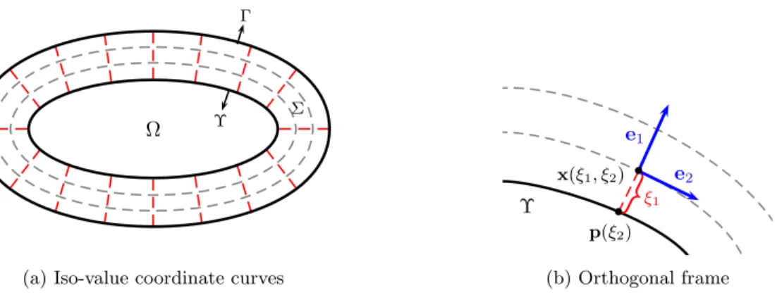
spatial dimension d is equal to 2 or 3. For the modified problem, the fields are governed by system (1) only inside the truncated domain Ω⊂ Rd, which is surrounded with the PML Σ (see e.g. Fig. 1a).

The time-harmonic PML formulations are obtained from the original equations by stretching a spatial coordinate in the complex plan, which introduces a directional damping of waves. In order to deal with

Ω Υ

Γ

Σ

(a) Iso-value coordinate curves

• • p(ξ2) x(ξ1, ξ2) e1 e2 Υ ξ1 (b) Orthogonal frame

Figure 1: Curvilinear coordinates and local frame associated with the boundary Υ in two dimensions. The curves of iso-value coordinates are represented in Fig. (a). Gray curves are parallel. Red lines are straight and perpendicular to Υ. Fig. (b) shows the local frame and the radial coordinate ξ1.

generally-shaped truncated domains, this stretch is performed in a specific local coordinate system. With this strategy, first used by Teixeira and Chew [71], the truncated domain must be convex with a regularity condition on its boundary, and the PML thickness is constant. The time-dependent formulations are then obtained by defining supplementary fields and applying an inverse Fourier transform in time.

The local coordinate system is described in section 2.1. The time-harmonic and time-dependent PML formulations are derived in sections2.2and2.3, respectively.

2.1

Coordinate system associated with the domain boundary

We consider a local coordinate system defined in a layer Σ surrounding the domain Ω with a constant thickness δ. The system is based on lines (in two dimensions) or surfaces (in three dimensions) parallel and perpendicular to the interface Υ (Fig. 1a), which is assumed to be regular enough. This system has been used to derive PMLs [51,52,71,74] and absorbing boundary conditions [4].

In two dimensions, the interface Υ is a curve and the coordinate system is denoted (ξ1, ξ2). Since Ω is

convex, each point x(ξ1, ξ2) of the layer Σ has a unique closest point on Υ. We define the coordinate ξ1 as

the distance between the two points, while the coordinate ξ2 is given by a local parametrization of Υ. We

consider a coordinate patch of Υ defined as p :V ⊂ R → Υ. Each point of p(V) ⊂ Υ then is given by p(ξ2),

where ξ2∈ V. The coordinate patch is chosen in such a way that

dn dξ2

= κt, with t = dp dξ2

,

where n(ξ2) is the unit outward normal, t(ξ2) is a unit tangent vector and κ(ξ2) is the curvature of Γ at p(ξ2).

The coordinates ξ1 and ξ2 form an orthogonal curvilinear system, and the set of vectors (e1, e2) = (n, t)

constitutes an orthonormal frame. For each point of the layer Σ, we can then write x(ξ1, ξ2) = p(ξ2) + ξ1e1(ξ2),

which is illustrated in Fig. 1b.

The three-dimensional coordinate system (ξ1, ξ2, ξ3) is adapted from the two-dimensional version. For

each point of the layer Σ, the coordinate ξ1 is the distance with the closest point on the surface Υ, and

the coordinates ξ2 and ξ3 are provided by a local parametrization of Υ. We consider a coordinate patch

p : V ⊂ R2 _{→ Υ. Each point of p(V) ⊂ Υ then is given by p(ξ}

2, ξ3), where (ξ2, ξ3)∈ V. There exists a

coordinate patch that gives (see [4,28]) dn dξi = κiti, with ti= dp dξi , for i = 2, 3, (2)

where n(ξ2, ξ3) is the unit outward normal, t2(ξ2, ξ3) and t3(ξ2, ξ3) are two unit tangent vectors in the

principal directions and κ2(ξ2, ξ3) and κ3(ξ2, ξ3) are the principal curvatures of the surface Γ at p2(ξ2, ξ3).

The coordinates ξ1, ξ2 and ξ3 form an orthogonal curvilinear coordinate system, and the set of vectors

(e1, e2, e3) = (n, t2, t3) constitutes an orthonormal frame. For each point of the layer Σ, we can then write

x(ξ1, ξ2, ξ3) = p(ξ2, ξ3) + ξ1e1(ξ2, ξ3). (3)

In orthogonal curvilinear coordinates, system (1) can be written          ∂p ∂t + ρc 2_∏1 khk ( ∑ i ∂ ∂ξi ((∏ k̸=ihk ) ui )) = 0, ∂ui ∂t + 1 ρ 1 hi ∂p ∂ξi = 0, for i = 1, . . . , d (4)

where ui denotes a component of u in the coordinate system, and hi is the scale factor associated with the

coordinate ξi, which is defined by

hi= ∂x ∂ξi . (5)

The lower and upper bounds of summation and product symbols are 1 and d, respectively. For the sake of clarity, they are not written. Using the definition (5) together with equations (2) and (3) gives the scale factors for the three-dimensional coordinate system described in this section,

h1= 1,

h2= 1 + κ2(ξ2, ξ3) ξ1,

h3= 1 + κ3(ξ2, ξ3) ξ1.

2.2

Coordinate stretch and time-harmonic PML systems

         −ıωˆp + ρc2_∏1 khk ( ∑ i ∂ ∂ξi ((∏ k_̸=ihk ) ˆ ui )) = 0, −ıωˆui+ 1 ρ 1 hi ∂ ˆp ∂ξi = 0, for i = 1, 2, 3, (6)

where ω is the angular frequency and the hat ˆ denotes the Fourier transform in time. Both will be used to derive different time-dependent PML formulations in section2.3.

In a time-harmonic context, a classical way to derive PML systems from the original system consists in stretching one coordinate in the complex plane, where the coordinate corresponds to the direction where waves must be damped in the layer. In our case, this corresponds to replacing the real coordinate ξ1 ∈

[0, δ] with the complex one ˜ξ1 ∈ U, where U is a curve in the complex plane (Fig. 2). We consider the

parametrization of the curve ˜ ξ1(ξ1) = ξ1− 1 ıω ∫ ξ1 0 σ(ξ₁′) dξ′₁, with ξ1∈ [0, δ], (7)

where σ(ξ1) is the so-called absorption function, which is positive. The effect of the complex stretching with

this specific parametrization can be interpreted by considering the plane wave solution. For the original system (6), the plane wave solution reads

eı(k·x−ωt),

where the wave number k is related to the angular frequency through the dispersion relation ω = c∥k∥. Replacing ξ1with ˜ξ1 in this solution gives

ℜe ℑm

0 δ

• •

(a) Original medium

ℜe ℑm U 0 δ • • (b) PML medium Figure 2: Complex coordinate stretch of the radial coordinate ξ1.

with the damping factor

γ(ξ1) = 1 c k· e1 ∥k∥ ∫ ξ1 0 σ(ξ1′) dξ1.

Except grazing waves (i.e. k· e1= 0), all the plane waves supported by the original system are damped in

their direction of propagation. For outgoing plane waves (i.e. k· e1> 0), the damping factor is positive and

increases when ξ1 increases. By contrast, for ingoing plane waves (i.e. k· e1 < 0), the damping factor is

negative and increases when ξ1 decreases.

When replacing ξ1 with ˜ξ1 in the time-harmonic system (6), the partial derivative with respect to ξ1

becomes ∂ ∂ξ1 → ∂ ∂ ˜ξ1 = 1 1− σ/(ıω) ∂ ∂ξ1 ,

and the scale factors h2 and h3, which depend on ξ1, become

h2 → ˜h2= 1 + κ2ξ˜1,

h3 → ˜h3= 1 + κ3ξ˜1.

The other partial derivatives do not change, nor does the scale factor h1= 1. Nevertheless, it is convenient

to introduce the complex scale factor defined as ˜h1= 1− σ/(ıω). Indeed, the time-harmonic PML system

can then be written          −ıωˆp + ρc2_∏1 k˜hk ( ∑ i ∂ ∂ξi ((∏ k_̸=i˜hk ) ˆ ui )) = 0, −ıωˆui+ 1 ρ 1 ˜ hi ∂ ˆp ∂ξi = 0, for i = 1, 2, 3. (8)

An alternative PML system is obtained by defining the new unknowns

ˆ u⋆_i = ∏ k̸=ih˜k ∏ k̸=ihk ˆ ui, for i = 1, 2, 3.

System (8) then becomes            −ıωˆp + ρc2 ∏ khk ∏ k˜hk 1 ∏ khk ( ∑ i ∂ ∂ξi ((∏ k̸=ihk ) ˆ u⋆_i )) = 0, −ıωˆu⋆ i + 1 ρ hi ˜ hi Πk̸=i˜hk Πk̸=ihk 1 hi ∂ ˆp ∂ξi = 0, for i = 1, 2, 3. (9)

Both time-harmonic PML systems (8) and (9) have interpretations that are well-known in the electro-magnetics community. For system (8), the complex coordinate stretch corresponds to a change of the metric

of the space. In an orthogonal coordinate system, the original scale factors hi are indeed simply replaced

with the complex ones ˜hi (see e.g. [52,73,74]). The tensor form of system (9) reads

   −ıωˆp + ρc2_{α∇ · ˆu}⋆ = 0, −ıωˆu⋆ +1 ρM∇ˆp = 0,

where the scalar α and the second-order tensorM are defined by

α = ∏ khk ∏ kh˜k and M =∑ i hi ˜ hi ∏ k̸=ih˜k ∏ k̸=ihk (ei⊗ ei) .

This system is identical to the original one (system (1)), except that the (real) material parameters ρc2

and 1/ρ have been replaced with the complex parameter ρc2_{α and the anisotropic complex tensor M/ρ.}

The time-harmonic PML can then simply be interpreted as an anisotropic absorber with specific complex material properties [32,66,71]. The same material properties have been obtained for the Helmholtz equation by Matuszyk and Demkowicz [55] in a more general framework.

2.3

Time-dependent PML systems

Two time-dependent PML systems are obtained from the time-harmonic ones (8) and (9) by using an inverse Fourier transform in time. This transform can be performed thanks to the introduction of additional fields and equations. For the sake of clarity, we define the real functions

σ1= σ(ξ1), σ2= ¯κ2(ξ1, ξ2, ξ3) ¯σ(ξ1), (10) σ3= ¯κ3(ξ1, ξ2, ξ3) ¯σ(ξ1), (11) with ¯ κi(ξ1, ξ2, ξ3) = κi 1 + κiξ1 , with i = 2, 3, ¯ σ(ξ1) = ∫ ξ1 0 σ(ξ₁′) dξ₁′.

These functions allow us to rewrite the complex scale factors as ˜ hi= ( 1− σi ıω ) hi. (12)

Let us firstly consider system (8). By using equation (12), the second term of the first equation of system (8) successively becomes ρc2∏1 k˜hk ∑ i ∂ ∂ξi ((∏ k̸=i˜hk ) ˆ ui ) = ρc2∏1 k˜hk ∑ i [(∏ k_̸=i ( 1−σk ıω )) ∂ ∂ξi ((∏ k_̸=ihk ) ˆ ui ) +((∏_k̸=ihk ) ˆ ui ) _∂ ∂ξi (∏ k_̸=i ( 1−σk ıω ))] =∑ i ( 1−σi ıω )−1[_ρc2_∏1 khk ∂ ∂ξi ((∏ k̸=ihk ) ˆ ui )] +∑ i [ ρc2(∏_k(1−σk ıω )−1)uˆi hi ∂ ∂ξi (∏ k̸=i ( 1−σk ıω ))] =∑ i ( 1− σi σi−ıω ) [ ρc2∏1 khk ∂ ∂ξi ((∏ k̸=ihk ) ˆ ui )] +∑ i  ρc2 (−ıω) σi− ıω ∑ k_̸=i [ 1 σk− ıω ∂σk ∂ξi ] ˆ ui hi   .

Using the definitions of σ1, σ2, σ3 and h1, the second term can be simplified as ∑ i  ρc2 (−ıω) σi− ıω ∑ k̸=i [ 1 σk− ıω ∂σk ∂ξi ] ˆ ui hi   = ρc2uˆ1 (−ıω) σ1− ıω [ 1 σ2− ıω ∂σ2 ∂ξ1 + 1 σ3− ıω ∂σ3 ∂ξ1 ] + ρc2 (−ıω) (σ2− ıω)(σ3− ıω) [ ˆ u2 h2 ∂σ3 ∂ξ2 +uˆ3 h3 ∂σ2 ∂ξ3 ] = ρc2uˆ1 (−ıω) σ1− ıω [ σ1− σ2 σ2− ıω ¯ κ2+ σ1− σ3 σ3− ıω ¯ κ3 ] + ρc2 (−ıω) (σ2− ıω)(σ3− ıω) [ ˆ u2 h2 ∂σ3 ∂ξ2 +uˆ3 h3 ∂σ2 ∂ξ3 ] = ρc2uˆ1 [ − (−ıω) σ1− ıω (¯κ2+ ¯κ3) + (−ıω) σ2− ıω ¯ κ2+ (−ıω) σ3− ıω ¯ κ3 ] + ρc2 (−ıω)¯σ (σ2− ıω)(σ3− ıω) [ ¯ κ2 3 κ2 3 ˆ u2 h2 ∂κ3 ∂ξ2 +κ¯ 2 2 κ2 2 ˆ u3 h3 ∂κ2 ∂ξ3 ] =∑ i ( 1− σi σi−ıω ) (ˆqi+ ¯σˆri),

where we have introduced the additional fields ˆ q1=−ρc2(¯κ2+ ¯κ3)ˆu1, rˆ1= 0, ˆ q2= ρc2κ¯2uˆ1, rˆ2= ρc2 1 σ3− ıω ¯ κ2 3 κ2 3 ˆ u2 h2 ∂κ3 ∂ξ2 , ˆ q3= ρc2κ¯3uˆ1, rˆ3= ρc2 1 σ2− ıω ¯ κ2 2 κ2 2 ˆ u3 h3 ∂κ2 ∂ξ3 .

Defining the additional fields ˆ pi=− 1 σi− ıω [ ρc2∏1 khk ∂ ∂ξi ((∏ k̸=ihk ) ˆ ui ) + ˆqi+ ¯σˆri ] , for i = 1, 2, 3, system (8) can be rewritten as

                                     −ıωˆp + ρc2_∏1 khk ( ∑ i ∂ ∂ξi ((∏ k̸=ihk ) ˆ ui )) =−∑ i (σipˆi)− ∑ i (ˆqi+ ¯σˆri), −ıωˆui+ 1 ρ 1 hi ∂ ˆp ∂ξi =−σiuˆi, for i = 1, 2, 3, −ıωˆpi+ ρc2 1 ∏ khk ∂ ∂ξi ((∏ k̸=ihk ) ˆ ui ) =−(σipˆi+ ˆqi+ ¯σˆri), for i = 1, 2, 3, −ıωˆr2= ρc2 ¯ κ2 3 κ2 3 ˆ u2 h2 ∂κ3 ∂ξ2 − σ 3rˆ2, −ıωˆr3= ρc2 ¯ κ2 2 κ2 2 ˆ u3 h3 ∂κ2 ∂ξ3 − σ2rˆ3.

One equation can be removed by using ˆp =∑_ipˆi, as well as one term of the first equation since

∑

iqˆi= 0.

Using an inverse Fourier transform in time, we finally obtain the time-dependent PML system                                    ∂p ∂t + ρc 2_{∇ · u = −σ} 1p1− σ2p2− σ3(p− p1− p2)− ¯σ(r2+ r3), ∂u ∂t + 1 ρ∇p = − ∑ i σiuiei, ∂pi ∂t + ρc 2_∇ i· u = −σipi− qi− ¯σri, for i = 1, 2, ∂r2 ∂t = ρc 2_u 2 ¯ κ2 3 κ2 3 (e2· ∇κ3)− σ3r2, ∂r3 ∂t = ρc 2_u 3 ¯ κ2₂ κ2 2 (e3· ∇κ2)− σ2r3. (13)

with ui= ei· u, q1=−ρc2(¯κ2+ ¯κ3)u1, q2= ρc2¯κ2u1and

∇i· u

def.

= ∇ · (uiei). (14)

With this system, the governing equations of p and u are identical to the original ones, but with additional non-differential terms. The original equations are recovered if σ is equal to zero. This formulation has four supplementary differential equations: two with the differential operator of equation (14) and two ordinary differential equations. The latter involve the spatial variation of each principal curvature (κ2and κ3) in the

other principal direction (respectively, e3and e2). For a sphere, the curvature is constant and the fields r1

and r2are equal to zero. In two dimensions, only one supplementary partial differential equation is required.

We now consider system (9), which can be rewritten as            −ıωˆp + ρc2_∏1 khk ( ∑ i ∂ ∂ξi ((∏ k_̸=ihk ) ˆ ui )) =−ıω ( 1− ∏ k˜hk ∏ khk ) ˆ p, −ıωˆui+ 1 ρ 1 hi ∂ ˆp ∂ξi =−ıω ( 1− ˜ hi hi ∏ k_̸=ihk ∏ k̸=ih˜k ) ˆ ui.

For the sake of clarity, the superscript ⋆ _{has been removed. Using equation (12), the right-hand sides of}

these equations become

−ıω ( 1− ∏ k˜hk ∏ khk ) ˆ p =−ıω ( 1− ( 1−σ1 ıω ) ( 1−σ2 ıω ) ( 1−σ3 ıω )) ˆ p =− (∑_iσi) ˆp−(∑_i ∏ k̸=iσi ) _pˆ (−ıω)− ( ∏ iσi) ˆ p (−ıω)2, −ıω ( 1− ˜ hi hi ∏ k_̸=ihk ∏ k̸=i˜hk ) ˆ ui=−ıω ( 1−∏ 1− σi/(ıω) k̸=i(1− σk/(ıω))) ) ˆ ui =−ıω ∏ k̸=i(ıω_∏− σk)− ıω(ıω − σi) k_̸=i(ıω− σk) ˆ ui =−ıω ıω ( σi− ∑ k̸=iσk ) +∏_k̸=iσk ∏ k̸=i(ıω− σk) ˆ ui =− ( σi− ∑ k_̸=iσk ) (ˆvi+ ˆui)− (∏ k_̸=iσk ) ˆ wi,

where ˆvi and ˆwi have been introduced such that

ˆ vi+ ˆui= (ıω)2 ∏ k_̸=i(ıω− σk) ˆ ui= (ıω)2 (ıω)2− ıω(∑ k_̸=iσk ) +(∏_k̸=iσk ) ˆui, ˆ wi= ıω ∏ k̸=i(ıω− σk) ˆ ui= ıω (ıω)2_{− ıω}(∑ k_̸=iσk ) +(∏_k̸=iσk ) ˆui, which give −ıωˆvi=− (∑ k_̸=iσk ) (ˆvi+ ˆui) + (∏ k_̸=iσk ) ˆ wi, −ıω ˆwi=−(ˆvi+ ˆui).

finally obtain the system                            ∂p ∂t + ρc 2_∏1 khk ( ∑ i ∂ ∂ξi ((∏ k̸=ihk ) ui )) =− (∑_iσi) p−(∑_i ∏ k̸=iσi ) p(1)_{− (}∏ iσi) p (2)_, ∂ui ∂t + 1 ρ 1 hi ∂p ∂ξi =− ( σi− ∑ k̸=iσk ) (ui+ vi)−(∏_k̸=iσk ) wi, ∂p(1) ∂t = p, ∂vi ∂t =− (∑ k̸=iσk ) (ui+ vi) +(∏_k̸=iσk ) wi, ∂p(2) ∂t = p (1)_, ∂wi ∂t =−(vi+ ui).

The tensor form of this system reads                        ∂p ∂t + ρc 2_{∇ · u = − (σ} 1+ σ2+ σ3) p− (σ1σ2+ σ1σ3+ σ2σ3) p(1)− (σ1σ2σ3) p(2), ∂u ∂t + 1 ρ∇p = −A(u + v) − Bw, ∂p(1) ∂t = p, ∂v ∂t =−C(u + v) + Bw, ∂p(2) ∂t = p (1)_, ∂w ∂t =−(u + v), (15)

with the second-order tensors

A = (σ1− σ2− σ3)I1+ (−σ1+ σ2− σ3)I2+ (−σ1− σ2+ σ3)I3,

B = (σ2σ3)I1+ (σ1σ3)I2+ (σ1σ2)I3,

C = (σ2+ σ3)I1+ (σ1+ σ3)I2+ (σ1+ σ2)I3,

where Ii = ei⊗ ei. As in system (13), p and u are governed by the original equations where source terms

are added. By contrast, this formulation involves two scalar and two vectorial supplementary fields, which are governed by ordinary differential equations. Only one scalar field and one vector field are required in two dimensions.

In the remainder, systems (13) and (15) are respectively called the PML-PDE system and the PML-ODE system.

Interpretation and extension for domains with corners

Though the PML systems have been derived for convex domains with regular boundary, they can straight-forwardly be adapted for squared and cuboidal domains with edge and corner regions where layers overlap. Formula (12) is classically used to stretch scale factors in the Cartesian directions to derive PML for squared and cuboidal domains (see e.g. [72, 74]). Therefore, the PML systems (13) and (15) can be used as is for Cartesian PMLs, but each absorption function σi(xi) is chosen independently and corresponds to the

damping of waves in the corresponding Cartesian direction ei.

An analogy with the Cartesian PMLs provides a nice interpretation for the absorbing functions σ2 and

σ3 expressed in equations (10) and (11). They can be considered as absorption functions associated with

the principal directions, but they are due to the curvature of the domain boundary. They are equal to zero if the boundary is planar.

The validity of the PML systems (13) and (15) can also be extended to other convex domains having corners with right angles. For instance, they can deal with cylindrical domains having convex cross-sections. Let us consider a cylinder with the axis e3. In the lateral PML that surrounds the cylinder, the PML systems

are then simply obtained by considering that κ2is the curvature of the cross section and κ3→ 0 in relations

(10) and (11); e1 remains the radial direction and e2 is tangent the lateral surface and perpendicular to e3.

At the two extremities of the cylinder, the PMLs are planar and only σ3is non-zero. At the corner, σ1 and

Classification and mathematical properties

The derived PML-PDE system (13) and PML-ODE system (15) can be categorized into two well-known families of PMLs. The first family contains the B´erenger-like PML systems that are built using the

splitting-field technique of B´erenger [13] or the complex coordinate stretch technique [21,22]. These systems involve additional fields governed by differential equations with spatial partial derivatives (see e.g. [14, 23,24, 45–

47, 60]). The second family corresponds to PML systems based on frequency-dependent complex material properties [32, 66, 78] and written in the time-domain with supplementary ordinary differential equations [2,19,62]. Such PMLs are generally referred as uniaxial PMLs.

The mathematical properties of PMLs from both families have been studied in many works and are still an active field of research (see e.g. [1,2,9, 10,27, 31, 41,42, 48, 62]). For wave problems described with symmetric hyperbolic systems (e.g. acoustic system (1) and Maxwell’s equations), the PML systems derived with the original strategy of B´erenger are weakly hyperbolic, and lead to weakly well-posed problems [1,9]. By contrast, the uniaxial PML systems are symmetric hyperbolic and lead to strongly well-posed problems [2,42,62]. To our knowledge, only proofs of weak stability have been proposed for standard PML systems from both families [9, 12, 19]. This means that no exponentially growing modes are supported by the equations, but linear modes could pollute the solution in long-duration simulations. Since the PML systems studied in [9,12,19] correspond to planar versions of systems (13) and (15), the PML formulations proposed in this work will also suffer from the same long-time instability.

Let us note that modified PML formulations have been proposed to avoid any linear growing mode, and to improve the accuracy for problems involving evanescent and grazing waves. For instance, the so-called

complex frequency shifted PML formulations [50,65] are derived using a modified coordinate stretch, where new parameters are introduced. In the time domain, these formulations can be seen as generalizations of standard PML formulations with supplementary terms and equations. The formulations proposed in this work could be enriched using the modified coordinate stretch, but at the cost of larger PML systems and more expensive computations.

3

Numerical simulations

Both time-dependent PML formulations are tested by means of a three-dimensional benchmark where a spherical wavefront is propagated in a truncated domain. The computational domain is the half of an ellipsoid of revolution, whose shell is extended with a PML. The simulations are performed using discontinuous finite element schemes that are described in section 3.1. After the description of the benchmark in section 3.2, accuracy results are proposed to validate our implementation and performance results are discussed (section

3.3). An illustration of application is finally proposed in section3.4.

For the PML-PDE formulation (13), both fields ri are set to zero and the corresponding equations are

not computed. Since the domain has an axis of revolution, one of the principal curvatures is constant, and the corresponding field is equal zero. Setting the other field to zero is an approximation that corresponds to neglecting the effect of the spatial variation of the other principal curvature. With our specific benchmark, we have observed a posteriori that the performances of the formulation remain very good in comparison to the PML-ODE formulation, which is implemented without any approximation.

3.1

Discontinuous finite element schemes

We propose numerical schemes based on a nodal discontinuous Galerkin (DG) method for the PML sys-tems. The schemes are derived following a classical strategy for hyperbolic systems [44], with some further developments to discretize the supplementary equations.

The unknown fields are approximated on a spatial mesh of Ω made of non-overlapping polyhedral cells,

Ω =∪_k=1,...,KDk, where K is the number of cells and Dk is the kth cell. With the nodal DG method, each

scalar field and each Cartesian component of vector fields is approximated by piecewise polynomial functions, where discontinuities correspond to interfaces between elements. The discrete unknowns correspond to the

values of fields at the nodes of elements. Over each cell Dk, the approximation of any field q(x, t) can then be written as qk(x, t) = Nk ∑ n=1 qk,n(t) ℓk,n(x), ∀x ∈ Dk,

where Nk is the number of nodes over element k, qk,n(t) is the value of the field at node n, and ℓk,n(x) is

the multivariate Lagrange polynomial function associated with node n.

For both the original system (1) and the PML systems (13) and (15), the governing equations of p and u are discretized in the same manner. Multiplying these equations by test functions ˆp and ˆu, integrating the resulting equations over any cell Dk, and using integration by parts, we get the weak form

( ∂p ∂t, ˆp ) Dk −(ρc2u,∇ˆp)_D k+⟨fp, ˆp⟩∂Dk = (sp, ˆp)Dk, ( ∂u ∂t, ˆu ) Dk − ( p ρ,∇ · ˆu ) Dk +⟨fu, ˆu⟩_∂D k = (su, ˆu)Dk, with the fluxes

fp= ρc2nk· u,

fu= p ρnk,

where nk is the outward unit normal on the boundary ∂Dk. For both PML systems, sp and sucontain the

right-hand side terms of the governing equations of p and u. The discrete fields being discontinuous at the interface between elements, the fluxes are replaced by numerical fluxes which involve values of fields from both sides of interfaces. We choose the upwind fluxes

f_pnum= ρc2nk· { u}− cqpy, (16) f_unum= 1 ρnk { p}− c nk ( nk· q uy), (17)

where the mean{q}and the semi-jumpqqyof any field q are defined as { q}= q +_{+ q−} 2 , q qy= q +_{− q}− 2 .

The plus and minus subscripts denote values on the side of the neighboring and current cells, respectively. These fluxes are classically obtained by using a Riemann solver (see e.g. [44, 54]). At the external bound-ary, we use a first-order absorbing boundary condition (ABC) based on characteristics, which is simply implemented by taking the external values p+ and u+ equal to zero in the numerical fluxes (16)-(17).

For the PML-PDE system (13), the partial differential equations that govern the supplementary fields

p1and p2 are discretized by analogy with the governing equation of p. Multiplying these equations by test

functions, integrating over an element Dk of the layer Σ, and integrating by parts lead to the weak form

( ∂p1 ∂t , ˆp1 ) Dk −(ρc2e1(e1· u), ∇ˆp1 ) Dk+⟨fp1, ˆp1⟩∂Dk= (sp1, ˆp1)Dk, ( ∂p2 ∂t , ˆp2 ) Dk −(ρc2e2(e2· u), ∇ˆp2 ) Dk+⟨fp2, ˆp2⟩∂Dk= (sp2, ˆp2)Dk, where fp1 _{and f}p2 _{are defined as}

fp1= ρc 2_(n k· e1)(e1· u), fp2= ρc 2_(n k· e2)(e2· u),

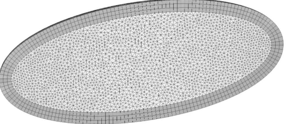
Figure 3: Geometry and mesh for the three-dimensional benchmark with a three-cells PML. This mesh is made of 58,396 tetrahedra in the truncated domain and 3× 6, 998 prisms in the layer.

and sp1 and sp2 contain the source terms written in the right-hand side of equations. Since system (13) is no longer strictly hyperbolic, we cannot use the Riemann solver to derive upwind fluxes. Noting the similitudes between fp and both fp1 and fp2, we propose to use the Lax-Friedrichs fluxes

f_pnum₁ = ρc2(nk· e1)(e1· { u})− cqp1 y , f_pnum₂ = ρc2(nk· e2)(e2· { u})− cqp2 y .

These fluxes are valid inside the layer Σ, but not at its external boundary Γ and at the interface Υ with the domain Ω. Indeed, because the supplementary fields are defined only inside the layer, we cannot use their semi-jumpsqp1

y

andqp2

y

on Υ and Γ. Fortunately, we note that nk =−e1 on Υ and nk = e1 on Γ. We

also have nk· e2= 0 on both surfaces. Therefore, we have fp1 = fp and fp2= 0 in both cases. We then use the numerical flux fnum

p instead of fpnum1 , and f

num

p2 is simply set to zero.

Since the supplementary equations of the PML-ODE system (15) do not involve spatial differential operators, the derivation of the scheme is straightforward. In addition to the above scheme for the governing equations of p and u, ordinary differential equations will be only local, at each node of each element, for the supplementary fields p(1), p(2), v and w. We use the same time-stepping scheme for both partial and ordinary differential equations.

3.2

Description of the benchmark

The computational domain Ω is the half of an ellipsoid, with axes of lengths 330 m (x−direction) and 120 m (y− and z−directions), respectively. A symmetry boundary condition is used in the section of the semi-ellipsoid, and the shell is extended with a PML Σ (Figure3). To generate the wavefront, a Gaussian pulse is prescribed as initial condition on the pressure,

p(x, 0) = e−r2/R2

with r = ∥x − x0∥, x0 = (−122.5 m, 0 m, 20 m) and R = 7.5 m, while the other fields are initially set to

zero. With this setting, the initial pressure is negligible inside the PML. We use the physical parameters

c = 1.5 km/s and ρ = 1 kg/m3_.

The mesh is made of tetrahedra in the truncated domain Ω and prisms in the layer Σ, with element sizes between 3 m and 5 m. The mesh of the layer is generated by extrusion. The main reason is that it can be automatically done for truncated domain of any shape with a regular enough boundary Υ. It does not require the analytic representation of the external boundary Γ of the layer. With an ellipsoidal domain, the external boundary Γ is not an ellipsoid (see e.g. [74]), and, to the best of our knowledge, no analytical representation is known. Ideally, a mesh with curvilinear elements should be used in order to exactly follow

the interface Υ and the boundary Γ that are curved. Elements with planar faces could be used with a lower computational cost, but the approximate polynomial representations of the surfaces introduce a geometric error. To reduce the global error, it is not clear if using curvilinear elements is computationally more efficient than using elements with planar faces and a thicker layer. In this paper, we consider only elements with planar faces.

We consider different thicknesses for the layer (1, 3 and 5 mesh cells) and both first-degree and second-degree basis functions. All the meshes are generated with Gmsh [33]. The time-stepping is made with the fourth-order Runge-Kutta scheme. The time step ∆t is equal to 0.05 ms and 0.025 ms for first-degree and second-degree basis functions, respectively.

Two alternative absorption functions σ(ξ1) are considered: the hyperbolic function σh and the shifted

hyperbolic function σsh, defined as

σh(ξ1) = c δ− ξ1 , σsh(ξ1) = c δ ξ1 δ− ξ1 .

It has been shown in previous works [16, 17, 57, 58] that both these functions do not require the tuning of parameters. In particular, we have shown [58] that σsh is a good choice for a discontinuous Galerkin

implementation with a Cartesian PML formulation similar to the PML-PDE system (13). Here, both functions are tested with both PML systems (13) and (15).

The PML formulations require to know the coordinate ξ1, the principal curvatures κ2 and κ3, and the

local orthonormal frame (e1, e2, e3). Both ξ1and e1are computed numerically by finding, in the initialization

of the simulation, the closest node belonging to the mesh of the surface Υ. To define the principal curvatures and the other vectors, we use the fact that the domain is an ellipsoid of revolution. Then, e2 belongs to

the plane tangent to Υ and is oriented towards one pole, and e3 is perpendicular to both e2 and e3. κ2

corresponds to the curvature of an ellipse [76],

κ2=

axay

[p2

x(ay/ax)2+ (p2y+ p2z)(ax/ay)2]3/2

,

and κ2is obtained from the Gaussian curvature G of an ellipsoid [77],

G = κ2κ3=

(axayaz)2

[(pxayaz/ax)2+ (pyaxaz/ay)2+ (pzaxay/az)2]2

.

In these formulas, ax, ay and az are the semi-axes of the ellipsoid and px, py and pz are the Cartesian

coordinates of p(ξ2, ξ3). Let us note that, in our case, ay= az.

3.3

Validation and comparison

Figure 4shows snapshots of the pressure p at different instants with a three-cells layer and the PML-PDE formulation. A spherical wave is generated by the initial pulse. As time goes by, the spherical wavefront reaches the PML with different angles of incidence, and propagates along the interface at a nearly grazing incidence. We observe that the spherical wave is not deformed near the interface, as we wished for, and the pressure is damped inside the layer.

The simulation is performed with different settings over the period [0 ms, 500 ms]. This includes a first phase where the wavefront is traveling in the truncated domain (before t = 200 ms) and a second phase where the wavefront has left the domain (after t = 200 ms). For all the settings, the difference between the numerical solution and the exact solution is quantified using the relative error defined as

Error(t) = ∫ Ω ( 1 2ρc2(pexact(t, x)− pnum(t, x)) 2 +ρ

2∥uexact(t, x)− unum(t, x)∥

2 ) dx ∫ Ω ( 1 2ρc2(pexact(0, x)) 2 +ρ 2∥uexact(0, x)∥ 2 ) dx ,

t = 0 ms

t = 50 ms

t = 100 ms

t = 150 ms

t = 200 ms

Figure 4: Snapshots of the solution of the three-dimensional benchmark at different instants. Colored surfaces are iso-surfaces of p(x, t). The inner and outer white surfaces correspond to the interior and exterior boundaries of the PML, respectively.

where the exact solution is given by pexact(t, x) = 1 2 ( r− ct r e −(r−ct)2_/R2 +r + ct r e −(r+ct)2_/R2 ) , uexact(t, x) = 1 2cρ [( R2 2r2 + r− ct r ) e−(r−ct)2/R2− ( R2 2r2 + r + ct r ) e−(r+ct)2/R2 ] x− x0 r .

The error corresponds to the ratio of the energy associated with the error fields to the energy associated with the initial fields in the truncated domain Ω.

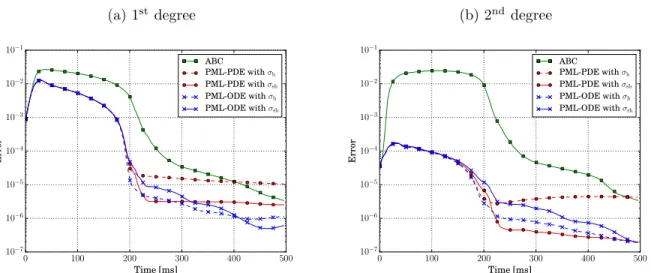
Figure5shows the time-evolution of the error when the absorbing boundary condition (ABC) and three-cells PMLs are used as truncation technique. Both first-degree and second-degree basis functions are tested. During the period [0 ms, 200 ms], all the PMLs exhibit a similar error for each polynomial degree. This error dramatically decreases when increasing the degree from one to two. By contrast, the error corresponding to the ABC is larger and stays at the same level (between 10−2 and 10−1) for both polynomial degrees. These observations are coherent with the properties of these truncation techniques. The considered ABC is only a first-order approximation that cannot simulate oblique outgoing waves without any reflection. The observed error then is dominated by the modeling error associated with spurious reflected waves already present at the continuous level. For the PMLs, the significant decay of error indicates that numerical errors dominate. In the second phase of the simulation (after t = 200 ms), the ABC error curves are decreasing and similar with both polynomial degrees. The error is dominated by the modeling error corresponding to the multiple reflections of the initial wavefront that are leaving the domain. With the PMLs, the error curves are in a quite large range (between 10−7 and 10−5) and have slightly different behaviors, which confirms that the kind of PML formulation and the absorption function impact the error. For both degrees, the error is far higher with the ABC than with the PMLs at the beginning of the second phase, but the ABC error goes under the error obtained with some PMLs at the end of the simulation. While the ABC error is dramatically decreasing during the second phase, the PML errors are only slightly decreasing or even slightly increasing. This phenomenon could be explained by the linear growing modes that can be generated inside the PML and that can pollute the long-duration solution (see the end of section3.3).

In order to compare the PML implementations, we now consider the mean value of the relative error over the period [250 ms, 500 ms], where the PMLs exhibit different errors. Figure 6 shows the mean error as function of the total runtime when using 2 Dual-Core Intel Xeon Processors L5420. All the one-cell PMLs provide similar errors for similar computational costs. For three-cells and five-cells layers, the PML-PDE implementation is more accurate with the shifted hyperbolic absorption function σsh than with the

(a) 1st degree (b) 2nd degree

0 100 200 300 400 500 Time [ms] 10−7 10−6 10−5 10−4 10−3 10−2 10−1 Error ABC PML-PDE with σh PML-PDE with σsh PML-ODE with σh PML-ODE with σsh 0 100 200 300 400 500 Time [ms] 10−7 10−6 10−5 10−4 10−3 10−2 10−1 Error ABC PML-PDE with σh PML-PDE with σsh PML-ODE with σh PML-ODE with σsh

Figure 5: Time-evolution of the error inside the domain Ω with the absorbing boundary condition (ABC) and three-cells PMLs. First-degree (a) and second-degree (b) basis functions are considered with both PML formulations and both absorbing functions.

(a) 1st degree (b) 2nd degree 0 1 2 3 4 5 6 Run time [h] 10−8 10−7 10−6 10−5 10−4 Mean error ABC PML-PDE with σh PML-PDE with σsh PML-ODE with σh PML-ODE with σsh 0 5 10 15 20 25 Run time [h] 10−8 10−7 10−6 10−5 10−4 Mean error ABC PML-PDE with σh PML-PDE with σsh PML-ODE with σh PML-ODE with σsh

Figure 6: Mean error over the period [250 ms, 500 ms] as a function of the runtime. The three points of each curve correspond to one-cell (left), three-cells (middle) and five-cells (right) layers.

hyperbolic one σh. This result is coherent with the conclusions of previous works with similar formulations

[57,58]. For the PML-ODE implementation, both functions provide quite similar results. σhis slightly better

than σsh with a three-cells layer, while the converse is true with a five-cells layer. Finally, the PML-PDE

implementation (with the shifted hyperbolic function) is more efficient than the PML-ODE. For a five-cells layer, it even provides a more accurate result with a smaller runtime.

3.4

Illustration of application

Our strategy is now illustrated by the scattering of a submarine placed in the center of the ellipsoidal domain. The submarine is approximately 120 m in length, and the dimensions of the ellipsoid are not changed. The PML-PDE is used together with the shifted hyperbolic absorption function σsh and the first-order ABC

to terminate the layer. The mesh is made of 183,707 tetrahedra (truncated domain) and 62,650 prisms (five-cells layer). First-degree basis functions are used. There are 7,450,112 degrees of freedom.

Figure 7 shows snapshots of the pressure p at different instants. The spherical wave generated by the initial pulse hits the front of the submarine, and creates perturbations in the pressure field. The wavefront propagates along the submarine and is nearly grazing at the boundary of the domain. The perturbations, as well as the primary spherical wave, have correctly left the front zone at t = 200 ms. These results have been obtained using 8 Dual-Core Intel Xeon Processors L5420. The total runtime was 1 h 40 min, corresponding to the period [0 ms, 200 ms] and to 8000 time steps.

4

Conclusion

This paper is dedicated to generalizing PML formulations for acoustic wave propagation with generally-shaped convex domains, which offers flexibility when choosing the shape of the computational domain. Our strategy is based on the complex stretch of a specific curvilinear coordinate in the time-harmonic equations, and on the use of supplementary differential equations to write the time-domain PML formulations.

Two time-dependent PML formulations have been derived for the pressure-velocity system. One formula-tion involves supplementary PDEs, while only ODEs are required for the other. Both have been implemented in a discontinuous Galerkin finite-element solver and tested with a three-dimensional benchmark. The best accuracy is observed with the PML-PDE formulation, despite an approximation made during the imple-mentation. That formulation is faster than the other, but the complete version requires the knowledge of supplementary geometrical information. In a more applicative context, we believe that all the required

t = 0 ms

t = 50 ms

t = 100 ms

t = 150 ms

t = 200 ms

Figure 7: Snapshots of the solution of the three-dimensional benchmark at different instants. Colored surfaces are iso-surfaces of p(x, t). The inner and outer white surfaces correspond to the interior and exterior boundaries of the PML, respectively

geometrical parameters could be evaluated numerically or provided by the underlying CAD software in an automatic manner.

The approach is quite general and offers a wide range of extensions. Since the PML equations are written at the continuous level, they can be implemented with other numerical methods. As explained at the end of section 2.3, the formulations can be adapted to deal with domains having corners, though they have been derived assuming that the domain border was regular enough. The formulations can also be improved using a complex coordinate stretch with a frequency shift [50,65].

Acknowledgements

This work was supported in part through the ARC grant for Concerted Research Actions (ARC WAVES 15/19-03), financed by the Wallonia-Brussels Federation, and by the Belgian Science Policy Office under grant IAP P7/02. Axel Modave was partially supported by an excellence grant from Wallonie-Bruxelles International (WBI). He was a Postdoctoral Researcher on leave with the F.R.S-FNRS. Jonathan Lambrechts was a Postdoctoral Researcher with the F.R.S-FNRS.

References

[1] S. Abarbanel and D. Gottlieb. A mathematical analysis of the PML method. Journal of Computational Physics, 134(2):357–363, 1997.

[2] S. Abarbanel and D. Gottlieb. On the construction and analysis of absorbing layers in CEM. Applied Numerical

Mathematics, 27(4):331–340, 1998.

[3] J. Alvarez, L. D. Angulo, A. R. Bretones, M. R. Cabello, and S. G. Garcia. A leap-frog discontinuous galerkin time-domain method for hirf assessment. IEEE Transactions on Electromagnetic Compatibility, 55(6):1250–1259, 2013.

[4] X. Antoine, H. Barucq, and A. Bendali. Bayliss-Turkel-like radiation conditions on surfaces of arbitrary shape.

Journal of Mathematical Analysis and Applications, 229(1):184–211, 1999.

[5] X. Antoine, A. Arnold, C. Besse, M. Ehrhardt, and A. Sch¨adle. A review of transparent and artificial boundary conditions techniques for linear and nonlinear Schr¨odinger equations. Communications in Computational Physics, 4(4):729–796, 2008.

[6] D. Appel¨o, T. Hagstrom, and G. Kreiss. Perfectly matched layers for hyperbolic systems: General formulation, well-posedness, and stability. SIAM Journal on Applied Mathematics, 67(1):1–23, 2006.

[7] U. Basu and A. K. Chopra. Perfectly matched layers for time-harmonic elastodynamics of unbounded domains: theory and finite-element implementation. Computer Methods in Applied Mechanics and Engineering, 192(11-12): 1337–1375, 2003.

[8] U. Basu and A. K. Chopra. Perfectly matched layers for transient elastodynamics of unbounded domains.

International Journal for Numerical Methods in Engineering, 59(8):1039–1074, 2004.

[9] E. B´ecache and P. Joly. On the analysis of B´erenger’s perfectly matched layers for Maxwell’s equations. ESAIM:

Mathematical Modelling and Numerical Analysis, 36(1):87–119, 2002.

[10] E. B´ecache and A. Prieto. Remarks on the stability of cartesian PMLs in corners. Applied Numerical Mathematics, 62(11):1639–1653, 2012.

[11] E. B´ecache, S. Fauqueux, and P. Joly. Stability of perfectly matched layers, group velocities and anisotropic waves. Journal of Computational Physics, 188(2):399–433, 2003.

[12] E. B´ecache, P. G. Petropoulos, and S. D. Gedney. On the long-time behavior of unsplit perfectly matched layers.

IEEE Transactions on Antennas and Propagation, 52(5):1335–1342, 2004.

[13] J.-P. B´erenger. A perfectly matched layer for the absorption of electromagnetic waves. Journal of Computational

Physics, 114(2):185–200, 1994.

[14] J.-P. B´erenger. Three-dimensional perfectly matched layer for the absorption of electromagnetic waves. Journal

of Computational Physics, 127(2):363–379, 1996.

[15] J.-P. B´erenger. Perfectly Matched Layer (PML) for Computational Electromagnetics. Morgan & Claypool, 2007. [16] A. Berm´udez, L. Hervella-Nieto, A. Prieto, and R. Rodr´iguez. An exact bounded perfectly matched layer for

time-harmonic scattering problems. SIAM Journal on Scientific Computing, 30(1):312–338, 2007.

[17] A. Berm´udez, L. Hervella-Nieto, A. Prieto, and R. Rodr´iguez. An optimal perfectly matched layer with un-bounded absorbing function for time-harmonic acoustic scattering problems. Journal of Computational Physics, 223(2):469–488, 2007.

[18] A. Berm´udez, L. Hervella-Nieto, A. Prieto, and R. Rodr´iguez. Perfectly matched layers for time-harmonic second order elliptic problems. Archives of Computational Methods in Engineering, 17(1):77–107, 2010.

[19] Z. Chen and X. Wu. Long-time stability and convergence of the uniaxial perfectly matched layer method for time-domain acoustic scattering problems. SIAM Journal on Numerical Analysis, 50(5):2632–2655, 2012. [20] W. C. Chew and Q. H. Liu. Perfectly matched layers for elastodynamics: A new absorbing boundary condition.

Journal of Computational Acoustics, 4(4):341–359, 1996.

[21] W. C. Chew and W. H. Weedon. A 3D perfectly matched medium from modified Maxwell’s equations with stretched coordinates. Microwave and Optical Technology Letters, 7(13):599–604, 1994.

[22] W. C. Chew, J. M. Jin, and E. Michielssen. Complex coordinate stretching as a generalized absorbing boundary condition. Microwave and Optical Technology Letters, 15(6):363–369, 1997.

[23] F. Collino and P. B. Monk. The perfectly matched layer in curvilinear coordinates. SIAM Journal on Scientific

Computing, 19:2061–2090, 1998.

[24] F. Collino and C. Tsogka. Application of the perfectly matched absorbing layer model to the linear elastodynamic problem in anisotropic heterogeneous media. Geophysics, 66(1):294–307, 2001.

[25] T. Colonius. Modeling artificial boundary conditions for compressible flow. Annual Review of Fluid Mechanics, 36:315–345, 2004.

[26] E. Demaldent and S. Imperiale. Perfectly matched transmission problem with absorbing layers: Application to anisotropic acoustics in convex polygonal domains. International Journal for Numerical Methods in Engineering, 96(11):689–711, 2013.

[27] J. Diaz and P. Joly. A time domain analysis of PML models in acoustics. Computer Methods in Applied Mechanics

and Engineering, 195(29):3820–3853, 2006.

[28] M. P. Do Carmo. Differential geometry of curves and surfaces. Prentice-hall Englewood Cliffs, 1976.

[29] B. Donderici and F. L. Teixeira. Conformal perfectly matched layer for the mixed finite element time-domain method. IEEE Transactions on Antennas and Propagation, 56(4):1017–1026, 2008.

[30] S. Dosopoulos and J.-F. Lee. Interior penalty discontinuous Galerkin finite element method for the time-dependent first order Maxwell’s equations. IEEE Transactions on Antennas and Propagation, 58(12):4085–4090, 2010.

[31] K. Duru. The role of numerical boundary procedures in the stability of perfectly matched layers. SIAM Journal

on Scientific Computing, 38(2):A1171–A1194, 2016.

[32] S. D. Gedney. An anisotropic perfectly matched layer-absorbing medium for the truncation of FDTD lattices.

IEEE Transactions on Antennas and Propagation, 44(12):1630–1639, 1996.

[33] C. Geuzaine and J.-F. Remacle. Gmsh: A 3-D finite element mesh generator with built-in pre-and post-processing facilities. International Journal for Numerical Methods in Engineering, 79(11):1309–1331, 2009.

[34] D. Givoli. Numerical Methods for Problems in Infinite Domains. Elsevier, 1992.

[35] D. Givoli. High-order local non-reflecting boundary conditions: a review. Wave Motion, 39(4):319–326, 2004. [36] D. Givoli. Computational absorbing boundaries. In Computational Acoustics of Noise Propagation in Fluids,

chapter 5, pages 145–166. Springer, Berlin, 2008.

[37] M. N. Guddati and K.-W. Lim. Continued fraction absorbing boundary conditions for convex polygonal domains.

International Journal for Numerical Methods in Engineering, 66(6):949–977, 2006.

[38] T. Hagstrom. Radiation boundary conditions for the numerical simulation of waves. Acta Numerica, 8:47–106, 1999.

[39] T. Hagstrom. Radiation boundary conditions for Maxwell’s equations: a review of accurate time-domain formu-lations. Journal of Computational Mathematics, 25:305–336, 2007.

[40] T. Hagstrom, D. Givoli, D. Rabinovich, and J. Bielak. The double absorbing boundary method. Journal of

Computational Physics, 259(0):220–241, 2014.

[41] L. Halpern and J. Rauch. Hyperbolic boundary value problems with trihedral corners. AIMS series in Applied

Mathematics, 2016.

[42] L. Halpern, S. Petit-Bergez, and J. Rauch. The analysis of matched layers. Confluentes Mathematici, 3(02): 159–236, 2011.

[43] F. D. Hastings, J. B. Schneider, and S. L. Broschat. Application of the perfectly matched layer (PML) absorbing boundary condition to elastic wave propagation. The Journal of the Acoustical Society of America, 100:3061, 1996.

[44] J. S. Hesthaven and T. Warburton. Nodal discontinuous Galerkin methods: algorithms, analysis, and applications, volume 54. Springer-Verlag New York, 2008.

[45] F. Q. Hu. On absorbing boundary conditions for linearized euler equations by a perfectly matched layer. Journal

of Computational Physics, 129(1):201–219, 1996.

[46] F. Q. Hu. Development of PML absorbing boundary conditions for computational aeroacoustics: A progress review. Computers & Fluids, 37(4):336–348, 2008.

equations based on the perfectly matched layer technique. Journal of Computational Physics, 227(9):4398–4424, 2008.

[48] B. Kaltenbacher, M. Kaltenbacher, and I. Sim. A modified and stable version of a perfectly matched layer technique for the 3-d second order wave equation in time domain with an application to aeroacoustics. Journal

of Computational Physics, 235:407–422, 2013.

[49] D. Katz, E. Thiele, and A. Taflove. Validation and extension to three dimensions of the B´erenger PML absorbing boundary condition for FD-TD meshes. IEEE Microwave and Guided Wave Letters, 4(8):268–270, 1994. [50] M. Kuzuoglu and R. Mittra. Frequency dependence of the constitutive parameters of causal perfectly matched

anisotropic absorbers. IEEE Microwave and Guided Wave Letters, 6(12):447–449, 1996.

[51] M. Lassas and E. Somersalo. Analysis of the PML equations in general convex geometry. Proceedings of the

Royal Society of Edinburgh: Section A Mathematics, 131:1183–1207, 2001.

[52] M. Lassas, J. Liukkonen, and E. Somersalo. Complex Riemannian metric and absorbing boundary condition.

Journal de Math´ematique Pures et Appliqu´ees, 80(7):739–768, 2001.

[53] J. W. Lavelle and W. C. Thacker. A pretty good sponge: Dealing with open boundaries in limited-area ocean models. Ocean Modelling, 20(3):270–292, 2008.

[54] R. J. LeVeque. Finite volume methods for hyperbolic problems, volume 31. Cambridge University Press, 2002. [55] P. J. Matuszyk and L. F. Demkowicz. Parametric finite elements, exact sequences and perfectly matched layers.

Computational Mechanics, 51(1):35–45, 2013.

[56] K. Meza-Fajardo and A. Papageorgiou. A nonconvolutional, split-field, perfectly matched layer for wave prop-agation in isotropic and anisotropicelastic media: Stability analysis. Bulletin of the Seismological Society of

America, 98(4):1811–1836, 2008.

[57] A. Modave, A. Kameni, J. Lambrechts, E. Delhez, L. Pichon, and C. Geuzaine. An optimum PML for scattering problems in the time domain. The European Physical Journal Applied Physics, 64, 11 2013.

[58] A. Modave, E. Delhez, and C. Geuzaine. Optimizing perfectly matched layers in discrete contexts. International

Journal for Numerical Methods in Engineering, 99(6):410–437, 2014.

[59] F. Nataf. A new approach to perfectly matched layers for the linearized Euler system. Journal of Computational

Physics, 214(2):757–772, 2006.

[60] I. M. Navon, B. Neta, and M. Y. Hussaini. A perfectly matched layer approach to the linearized shallow water equations models. Monthly Weather Review, 132(6):1369–1378, 2004.

[61] P. G. Petropoulos. Reflectionless sponge layers as absorbing boundary conditions for the numerical solution of Maxwell equations in rectangular, cylindrical, and spherical coordinates. SIAM Journal on Applied Mathematics, 60(3):1037–1058, 2000.

[62] A. N. Rahmouni. An algebraic method to develop well-posed PML models: Absorbing layers, perfectly matched layers, linearized Euler equations. Journal of Computational Physics, 197(1):99–115, 2004.

[63] C. Rappaport. Interpreting and improving the PML absorbing boundary condition using anisotropic lossy mapping of space. IEEE Transactions on Magnetics, 32(3):968–974, 1996.

[64] J. A. Roden and S. D. Gedney. Efficient implementation of the uniaxial-based PML media in three-dimensional nonorthogonal coordinates with the use of the FDTD technique. Microwave and Optical Technology Letters, 14 (2):71–75, 1997.

[65] J. A. Roden and S. D. Gedney. Convolutional PML (CPML): An efficient FDTD implementation of the CFS-PML for arbitrary media. Microwave and Optical Technology Letters, 27(5):334–338, 2000.

[66] Z. S. Sacks, D. M. Kingsland, R. Lee, and J.-F. Lee. A perfectly matched anisotropic absorber for use as an absorbing boundary condition. IEEE Transactions on Antennas and Propagation, 43(12):1460–1463, 1995. [67] K. Schmidt, J. Diaz, and C. Heier. Non-conforming Galerkin finite element methods for local absorbing boundary

conditions of higher order. Computers & Mathematics with Applications, 70(9):2252–2269, 2015.

[68] F. Teixeira, K.-P. Hwang, W. Chew, and J.-M. Jin. Conformal PML-FDTD schemes for electromagnetic field simulations: A dynamic stability study. IEEE Transactions on Antennas and Propagation, 49(6):902–907, 2001. [69] F. L. Teixeira and W. C. Chew. PML-FDTD in cylindrical and spherical grids. IEEE Microwave and Guided

Wave Letters, 7(9):285–287, 1997.

[70] F. L. Teixeira and W. C. Chew. Systematic derivation of anisotropic PML absorbing media in cylindrical and spherical coordinates. IEEE Microwave and Guided Wave Letters, 7(11):371–373, 1997.

[71] F. L. Teixeira and W. C. Chew. Analytical derivation of a conformal perfectly matched absorber for electro-magnetic waves. Microwave and Optical Technology Letters, 17(4):231–236, 1998.

[72] F. L. Teixeira and W. C. Chew. Unified analysis of perfectly matched layers using differential forms. Microwave

and Optical Technology Letters, 20(2):124–126, 1999.

[73] F. L. Teixeira and W. C. Chew. Differential forms, metrics, and the reflectionless absorption of electromagnetic waves. Journal of Electromagnetic Waves and Applications, 13(5):665–686, 1999.

[74] F. L. Teixeira and W. C. Chew. Complex space approach to perfectly matched layers: a review and some new developments. International Journal of Numerical Modelling-Electronic Networks Devices and Fields, 13