HAL Id: tel-01596030
https://tel.archives-ouvertes.fr/tel-01596030
Submitted on 27 Sep 2017HAL is a multi-disciplinary open access archive for the deposit and dissemination of sci-entific research documents, whether they are pub-lished or not. The documents may come from teaching and research institutions in France or abroad, or from public or private research centers.
L’archive ouverte pluridisciplinaire HAL, est destinée au dépôt et à la diffusion de documents scientifiques de niveau recherche, publiés ou non, émanant des établissements d’enseignement et de recherche français ou étrangers, des laboratoires publics ou privés.
networks for the degradation of civil infrastructures and
other applications
Alex Kosgodagan
To cite this version:
Alex Kosgodagan. High-dimensional dependence modelling using Bayesian networks for the degrada-tion of civil infrastructures and other applicadegrada-tions. Probability [math.PR]. Ecole nadegrada-tionale supérieure Mines-Télécom Atlantique, 2017. English. �NNT : 2017IMTA0020�. �tel-01596030�
Alex K
OSGODAGAN
-D
ALLA
T
ORRE
Mémoire présenté en vue de l’obtention du
grade de Docteur de l’École nationale supérieure Mines-Télécom Atlantique Bretagne Pays de la Loire
sous le sceau de l’Université Bretagne Loire
École doctorale : Sciences et technologies de l’information et mathématiques
Discipline : Mathématiques appliquées et applications des mathématiques, section CNU 26 Unité de recherche : Laboratoire des Sciences du Numérique de Nantes (LS2N)
Soutenue le 26 juin 2017 Thèse n° : 2017IMTA0020
High-dimensional dependence modelling using
Bayesian networks
for the degradation of civil infrastructures and other applications
JURY
Président : M. Christophe BÉRENGUER, Professeur des Universités, Grenoble INP Rapporteurs : M. Roger COOKE, Professor Emeritus, Resources for the Future
M. Laurent BOUILLAUT, Chargé de Recherche – HDR, IFSTTAR Examinateurs : M. Philippe LERAY, Professeur des Universités, Polytech Nantes
M. Laurent TRUFFET, Maître assistant – HDR, IMT Atlantique
M. Wim COURAGE, Senior Researcher, Structural Reliability, TNO Invité : M. Thomas G. YEUNG, Maître Assistant, IMT Atlantique
Directeur de thèse : M. Bruno CASTANIER, Professeur des Universités, Université d’Angers Co-directeur de thèse : M. Oswaldo MORALES-NÁPOLES, Assistant Professor, TU Delft
First of all, I would like to deeply thank all my supervisors B. Castanier, O. Morales-Napoles and T. G. Yeung, for their support, insight and the way each contributed to (hopefully) shape me as a young and autonomous researcher throughout this three-year journey as well as for their invaluable advice and encouragement. I am very grateful for the many opportunities they gave me to attend scientific conferences and for introducing me to their research groups. Special thanks goes to W. Courage for his kindness and commitment taking a significant part in my supervision as well.
Second of all, I want to thank both my Dutch and French colleagues many of whom became good friends throughout the past years. Starting with the Dutch side, thank you Wiebke, George and Dominik for the time we spent as young PhD together sharing Oswaldo as supervisor. Then, the "TNOers", thank you Nadieh, Johan, Laura, Adrii, Jos, Siska, Tineke, Yvonne and many others I am probably forgetting. From the French side, thank you Axel, Juliette, Quentin, Fabrice, Yuan and his chinese folks, Gilles, Guillaume, Naly, Laurent, Chams, Olivier, Dominique, Fabien, Hélène, Isabelle and Anita for integrating me with kindness into the team. Also, a thank you to the people I enjoyed sharing my office with, Alan, Lori, Rui, Agri and Iwan.
Besides the friends I made along the way, those whom I share so many great mem-ories with and being around for a very long time now, I would like to thank you Pop, Louis, Eloi, Kevin, Julie L., Camille B., Julie M., Camille F., Hélène, Caroline, Jerome, Alexis, Etienne,...
support and always had faith in me. I want to thank my uncles Pietro and Ruggero, my aunt Palma, my brother Sébastien and my wonderful mom.
1 Résumé 1
1.1 Introduction . . . 1
1.2 Résumé des travaux . . . 5
1.3 Conclusion . . . 9
2 Introduction 13 2.1 Context & motivation . . . 13
2.2 Bayesian networks . . . 19
2.2.1 Preliminaries on graphs. . . 19
2.2.2 Directional separation and conditional independence . . . 20
2.3 Outline of the thesis . . . 22
3 Non-parametric Bayesian network to assess crack growth prediction for steel bridges 29 3.1 Introduction . . . 29
3.2 Description of the detail. . . 32
3.3 Dependence model . . . 34
3.4 Sample-based conditioning for the monitored section . . . 37
3.5 Conclusion . . . 40 i
4 Expert judgment in life-cycle degradation and maintenance modelling for
steel bridges 43
4.1 Introduction . . . 44
4.2 Degradation modelling for orthotropic steel bridges . . . 46
4.3 Structured Expert Judgment . . . 50
4.3.1 Data on fatigue cracking . . . 53
4.3.2 Results . . . 54
4.3.3 Robustness tests . . . 57
4.3.4 Discussion . . . 59
4.4 Conclusions & perspectives. . . 60
5 A two-dimension dynamic Bayesian network for large-scale degradation modelling with an application to a bridges network 61 5.1 Introduction . . . 62
5.2 Deterioration framework . . . 66
5.2.1 Markov Chain . . . 66
5.2.2 Covariate-DBN . . . 69
5.2.3 Network Sensitivity Analysis. . . 72
5.3 Parametrization through Structured Expert Judgment . . . 74
5.3.1 Cooke’s model for eliciting expert opinions . . . 74
5.3.2 Calibration of pi,j . . . 75
5.4 Bridge Network Application . . . 78
5.4.1 Dependence structure . . . 80
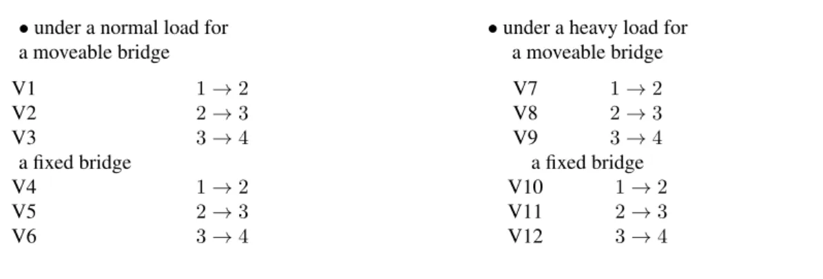
5.4.2 Traffic and load data . . . 81
5.4.3 Elicitation results . . . 83
5.5 Numerical experiment . . . 85
6 Representing k-th order Markov processes as a dynamic non-parametric
Bayesian network 95
6.1 Introduction . . . 95
6.2 Non-parametric Bayesian networks. . . 100
6.3 Dependence framework for a k-th order Markov process . . . 102
6.4 Representing Markov processes as a dynamic NPBN . . . 105
6.5 Conditioning . . . 109
6.6 Conclusion . . . 118
7 Conclusions 119 7.1 Perspectives . . . 123
Appendices 127
A Structured Expert Judgment 129
List of Tables 143
List of Figures 145
Résumé
Contents
1.1 Introduction . . . 1
1.2 Résumé des travaux . . . 5
1.3 Conclusion . . . 9
1.1
Introduction
Dans les domaines de la fiabilité et de la sûreté structurelle, l’exemple du réseau routier hollandais met en avant la complexité d’une part, et la nécessité d’autre part, de pouvoir modéliser les dynamiques d’un tel réseau. En effet, cet enchevêtrement de voies ne possède pas moins de 3200 kilomètres de routes référencées dont 2200 kilomètres d’entres elles font partie du réseau autoroutier. Au sein de ce réseau de transport, on compte approximativement 3000 ouvrages d’art. Dans ce contexte, l’objectif majeur pour les gestionnaires est de maintenir le réseau à un niveau satisfaisant des critères de sécurité et de confort. Toutefois, les facteurs rendant la tâche ardue de gérer un si vaste réseau sont multiples. Concernant la fiabilité des ponts routiers, ceux-ci incluent pêle-mêle, des innovations dans leur design et leur construction, l’évolution du trafic routier
conduisant à des dynamiques changeantes au niveau du poids auxquelles les ponts sont soumis, les changements climatiques, etc. Une observation générale sur laquelle cette thèse s’appuie est que ces facteurs exhibent de l’aléa.
L’émergence d’approches purement probabilistes se réfèrent souvent aux travaux deAbdel-Hameed[1975] où un processus gamma à pour la première fois été employé pour modéliser l’usure d’un composant. Depuis, une myriade de modèles s’appuyant partiellement ou totalement sur des méthodes probabilistes ont été développés.
Les travaux présentés dans cette thèse ont pour objectif de modéliser des prob-lèmes de dégradation d’infrastructures en grandes dimensions dans un cadre proba-biliste. Les réseaux Bayésiens (RB) répondent à ces critères. Ils proposent une com-préhension intuitive des relations entre les nœuds du graphes au travers de dépendances (in)conditionnelles. La littérature existante dénote une attractivité grandissante quant à l’utilisation des RB en fiabilité [Weber et al.,2012]. Par ailleurs, les RB se basent sur la version graphique de la propriété de Markov s’exprimant par les relations de dépen-dances conditionnelles. À l’instar des RB, les processus de Markov ont acquis une légitimité dans leur utilisation en fiabilité et sûreté structurelle pour les ouvrages d’art [Kallen,2007].
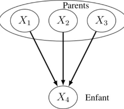
Plus formellement, un RB est un graphe orienté acyclique fournissant une représen-tation compacte d’une distribution de probabilité d’un ensemble de variables aléatoires (X1, ..., Xn) sous la forme de distributions conditionnelles. En utilisant des notions
X1 X2 X3
X4
Parents
Enfant
basiques de probabilité, à savoir la formule des probabilités totales, la densité jointe de quatre variables aléatoires peut s’écrire
f (x1, x2, x3, x4) = f (x1) 4
Y
i=2
f (xi|x1...xi−1) (1.1)
Les prédécesseurs directs d’un nœud Xi sont appelés parents et l’ensemble de tous
les parents de Xi s’écrit P a(Xi). À chaque variable aléatoire est associée une
prob-abilité conditionnelle de cette variable sachant ses parents, fXi|XP a(Xi), i = 1, ..., 4.
L’équation (1.1) appliquée au RB représenté en Fig.1.1peut ainsi être simplifiée grâce aux propriétés de dépendance conditionnelles supposées par les RB :
f (x1, x2, ..., xn) = 4
Y
i=1
f (xi|xP a(i)) (1.2)
Il existe plusieurs classes de RB. Selon la classe considérée, la paramétrisation d’un RB diffère. Nous nous sommes concentrés dans ces travaux en particulier sur deux d’entre elles. La première est la classe de RB dynamique discrète [Dagum et al.,1992,Murphy,
2002] où les relations de dépendance s’expriment par des probabilités conditionnelles classiques. La dimension dynamique intervient en termes de transitions temporelles en-tre chaque nœud. Cependant, pour cette classe la quantification du RB croît de manière exponentielle ayant pour paramètres le degré1 de chaque nœud ainsi que leur nombre d’états. Il est toutefois utile de mentionner que cette complexité peut être atténuée en générant de manière systématique les probabilités conditionnelles concernant les rela-tions temporelles nœud-à-nœud.
La seconde classe de RB est la classe des RB non-paramétrique (RBNP) [ Kurow-icka and Cooke, 2005]. À titre comparatif, les RBNP peuvent comprendre aussi bien des variables discrètes, continues et même un mélange continu-discret. Cependant, la
plus grande différence réside dans l’expression de la dépendance probabiliste. Celle-ci se traduit par des corrélations conditionnelles de rang et copules conditionnelles bi-variées associées à chaque arrête. Les copules ne nécessitant souvent que très peu de paramètres, e.g., un seul paramètre pour la copule Gaussienne, les RBNP se révèlent être peu couteux. Toutefois, les RBNP se limitent à une utilisation statique. En effet, aucune caractéristique temporel n’a été étudiée mis à part de manière marginale dans les travaux deMorales-Napoles and Steenbergen [2014]. Une partie des travaux de cette thèse s’attache donc à construire un cadre dynamique dans lequel les RBNP s’inscrivent. En pratique, la paramétrisation est effectuée à l’aide de données. Les jugements d’experts peuvent toutefois également être employés si les données sont insuffisantes ou de qualité ne permettant pas de les exploiter. Dans cette thèse, nous explorons un scénario nécessitant de paramétrer un RB discret dynamique et pour lequel les données disponibles sont insuffisantes. Nous employons la méthode de Cooke afin de combler ce déficit [Cooke,1991]. Comme nous l’avons précédemment évoqué, la quantification d’un RB dynamique est très couteuse et il serait par conséquent impossible d’avoir recours aux jugements d’experts afin de résoudre ce problème. Le choix d’utiliser un RBNP est d’autant plus renforcé qu’il est de plus en plus courant d’obtenir des données de corrélations conditionnelles de rang auprès d’experts [Werner et al.,2017].
En complément de leur qualité à traduire et organiser des problèmes hautement di-mensionnels, les RB possèdent également un autre avantage communément appelé in-férenceou update Bayésien. Concrètement, l’inférence consiste à calculer la distribu-tion de certains nœuds pour lesquels aucune informadistribu-tion n’est connue sachant la valeur d’autres nœuds du RB. L’inférence peut être effectuée aussi bien de "haut en bas" (diag-nostique) que de "bas en haut" (prédiction). Cette propagation d’information s’effectue encore une fois de manière différente selon que l’on traite les RB dynamiques ou les RBNP. D’un côté, l’inférence pour les RB dynamiques exige la résolution d’intégrales multidimensionnelles dont la valeur croit exponentiellement [Pearl, 1988]. D’un autre
côté, les RBNP permettent d’accomplir l’update Bayésien de manière analytique tant que la copule Gaussienne est supposée. Si la loi jointe est donnée par une autre copule, le RBNP est discrétisé et le problème d’inférence retombe dans le cadre discret.
1.2
Résumé des travaux
Le Chapitre32 développe un modèle de prédictions de fissurations d’acier dues au
phénomène de fatigue pour des ouvrages d’arts autoroutiers. L’objectif est d’exploiter des données provenant d’un système installé à un point sensible du pont. Ceci permet de formuler des prédictions pour les autres points du pont ne bénéficiant pas de don-nées. Le modèle requiert deux composantes sous-jacentes afin d’évaluer la durée de vie restante du pont. Premièrement, le mécanisme de fracturation élastique linéaire ainsi que le type de fissuration pouvant apparaitre sont présentés en Section3.2. Deuxième-ment, la Section3.3 décrit le cadre de dépendance probabiliste où un réseau Bayésien non-paramétrique est proposé. Le RBNP a pour but d’exploiter les corrélations entre les variables régissant le modèle à travers les différents points sensibles du pont ayant des caractéristiques identiques. Le but est de tirer parti de ces corrélations afin de propager les informations venant du système de monitoring vers les sections n’étant pas moni-torées.
Le cadre proposé par le RBNP nous permet par la suite d’effectuer des analyses de sensibilité sur l’ensemble des variables du modèle en Section 3.4. Les incertitudes au-tour des prédictions de fissurations sont réduites en conditionnant par échantillonnage Monte Carlo et en ne conservant que les simulations correspondant aux données de mon-itoring. En conséquence, nous avons pu mettre en évidence des différences d’inférence significatives concernant les variables régissant le modèle.
Le Chapitre43présente l’analyse des données d’experts obtenues par la méthode de 2. Ce Chapitre est extrait de l’article deAttema et al.[2016].
Cooke afin de partiellement paramétrer le modèle introduit au Chapitre5. Le Chapitre débute en présentant dans ses grandes lignes le modèle de dégradation, qui est encore un problème de fissuration d’acier, en Section4.2. La Section4.3énonce la méthodolo-gie de Cooke et définit les deux métriques permettant de classer les experts, i.e., les mesures de calibration et d’information. Ces métriques sont calculées à partir de vari-ables de calibration qui sont elle-mêmes construites à partir de données existantes rel-atives à des mesures de fissuration présentés en Section4.3.1. Les résultats de la per-formance des experts sont présentées en Section4.3.2 avançant, d’un côté, les scores médiocres de calibration obtenus pour chaque expert. Ceci étant probablement dû au faible nombre d’experts (3). D’autre part, la valeur combinée du score de calibration est très satisfaisante. Ce même score est substantiellement amélioré après que des tests de robustesse sont effectués et décrit en Section4.3.3. Les observations majeures de juge-ment d’experts sont en premier lieu une grande incertitude exprimée dans l’évaluation de probabilités. Deuxièmement, la pertinence des variables de calibration est abordée, notamment par rapport aux variables nécessitant de paramétrer le modèle. Ces remar-ques sont énumérées et discutées en Section4.3.4.
Le Chapitre 54 introduit le modèle intitulé réseau Bayésien dynamique co-varié (RBDC). L’objectif est de modéliser la dégradation d’un réseau d’ouvrages d’art dans scénario où les données de détérioration sont limitées. Le modèle de dégradation est présenté en Section5.2 où un processus de Markov à temps discret est proposé pour décrire la détérioration de chaque élément constituant le réseau. La Section5.2.1 dé-taille l’insertion de co-variables dans les probabilités de transitions qui rendent ces tran-sitions dynamiques. Dans le but de connecter les éléments du réseau, le RBDC est présenté en Section 5.2.2 où les ensembles des graphes et des probabilités condition-nelles sont donnés explicitement. Le modèle ainsi construit décrit un réseau Bayésien dynamique à deux dimensions, où la seconde dimension est exprimée par la relation
tre co-variables. Une méthodologie est proposée en Section5.2.3afin d’étudier la sen-sibilité du RBDC lorsque l’on effectue l’inférence. Cette méthodologie est motivée par la possible explosion combinatoire du réseau, qui plus est par l’ajout de cette seconde dimension. Deux configurations d’inférence sont proposées qui visent à être représen-tatives de l’ensemble des combinaisons existantes
La paramétrisation du modèle est ensuite discutée en Section 5.3. Nous rappelons que les résultats de jugement d’experts décrit au Chapitre 4sont implémentés afin de quantifier à la fois des probabilités de transitions du processus de Markov, ainsi que probabilités conditionnelles requises par le RBDC. La Section5.3.1rappelle brièvement la méthode de Cooke et ses objectifs. En Section5.3.2, les développements permettant la quantification des probabilités de transitions sont exhibés au travers de temps moyen de premier passage. La Section5.4présente le cas d’un problème de détérioration pour un réseau d’ouvrages d’art où le mécanisme latent de dégradation considéré consiste en l’apparition de fissurations se propageant dans le tablier due à la fatigue. Le RBDC est choisi comme méthodologie dans ce contexte où la structure de dépendance et le choix des co-variables sont décrit en Section 5.4.1. Les co-variables choisies représentent la densité du trafic et la sollicitation en poids induit par le trafic sur l’ouvrage d’art, étant les principales causes endogènes du mécanisme de fatigue. Les données de terrain permettant de quantifier ces deux co-variables sont discutées en Section 5.4.2. Les résultats de sortie du jugement d’experts sont combinés avec ces mesures de trafic et de poids afin d’obtenir in fine les matrices de transitions Markoviennes et de temps moyen de premier passage, ainsi que les courbes de probabilités de survie des ponts. Ces résultats sont décrit en Section5.4.3.
La Section 5.5 illustre différentes expérimentations utilisant les métriques de sen-sibilité afin d’étudier la manière dont le RBDC réagit. Nous avons d’abord observé que l’insertion cumulative d’information domine au détriment d’une configuration où l’insertion est individuellement réalisée au cours du temps. Par ailleurs, la sensibilité
de l’information décroît en temps, quelque soit la manière dont l’information a été in-troduite (cumulative ou bien individuelle). Par conséquent, il serait privilégié d’adopter une surveillance du réseau accrue à des périodes précoces.
Le Chapitre6traite de la démonstration théorique qu’un processus de Markov d’ordre k peut être représenté comme un RB non-paramétrique dynamique. Une définition formelle du RBNP est tout d’abord formulée en Section 6.2. Les conditions néces-saires et suffisantes afin de caractériser la partie probabiliste d’un RBNP sont données. Il s’agit des distributions marginales associées à chaque nœud, l’ensemble des copules conditionnelles bivariées et l’ensemble des corrélations conditionnelles de rang asso-ciées à chaque arrête du graphe.
Les copules conditionnelles sont présentées en Section 6.3 s’inscrivant spécifique-ment dans le cadre du processus Markovien d’ordre k. Le concept de la copule tem-porelle est présenté, i.e., la copule extraite de n’importe quel processus stochastique à deux pas de temps différents. Des explications concernant la relation entre copules et probabilités conditionnelles sont également indiquées. Nous fournissons de manière ex-plicite la relation entre la mesure d’auto-corrélation pour un processus stochastique et la formulation de corrélations conditionnelles de rang.
Le corps de la Section 6.4 développe la preuve de la représentation d’un proces-sus Markovien d’ordre k comme RBNP dynamique. Le théorème que nous énonçons s’appuie sur les travaux deJoe[1996] concernant les constructions de copules bivariées (pair-copula constructions), mais aussi sur les travaux récentsBauer and Czado[2016] sur la formulation de la loi jointe d’un RBNP en termes de copules conditionnelles bivariées. Une procédure résumant étape par étape les éléments clés du théorème est fournie en fin de Section.
La Section 6.5 exhibe la factorisation de distributions marginales multidimension-nelles pour des ensembles de nœuds. L’idée étant d’étudier l’expression analytique des distributions conditionnelles apparaissant dans l’expression des copules conditionnelles
bivariées. Deux cas sont traités. Le premier aborde celui où aucune paire de nœuds de l’ensemble de conditionnement n’a une longueur supérieure à l’ordre k du processus de Markov. La longueur ici représente la différence ordinale entre chaque nœud. Le sec-ond cas traite la configuration complémentaire. Cette séparation en deux cas provient de la capacité à séparer les ensembles de nœuds en utilisant la propriété de k-dépendance conditionnelle de Markov. Deux lemmes sont présentés subséquemment et résument ces découvertes. L’algorithme implémentant les deux lemmes est également décrit. Sa complexité est abordée et nous conjecturons qu’il performe mieux que celui deBauer and Czado[2016]. Enfin, nous illustrons notre approche globale au travers d’un exem-ple centré autour du mouvement Brownien.
1.3
Conclusion
Cette thèse s’est attelée à étudier des problèmes de dégradation, notamment celui du mécanisme de fissuration due à la fatigue, en grandes dimensions à travers les réseaux Bayésiens. L’approche globale prônée dans ce manuscrit possède deux composantes complémentaires en ce sens qu’elle fait appel à des outils à la fois probabilistes et statis-tiques. La raison ayant motivé ce choix est double. Tout d’abord, les systèmes se sont complexifiés au cours des dernières décennies et la part d’incertain relative à la fiabilité et la sûreté s’est accrue en conséquence. De plus, l’identification et la quantification de leur causes, possédant souvent de l’incertain aussi, apparaissent de plus en plus difficile. Deuxièmement, l’accessibilité grandissante de grands ensembles de données tendraient à se diriger vers des méthodes statistiques. Nous avons mis en lumière que les RB se révèlent être une approche versatile au sein de laquelle les angles probabilistes et statis-tiques s’entrelacent. Leur efficacité dans le domaine de la modélisation de dégradation pour des ouvrages d’arts a été testée et validée dans les Chapitres 3, 4 et 5. Bien qu’aucune application orientée à la fiabilité n’ait été présentée dans le Chapitre6, nous
pouvons affirmer que l’approche développée est dans la lignée des chapitres précédant concernant des considérations de détérioration et leur efficience. Un argument immédiat serait que quelque soit la classe de RB considérée, la propriété de Markov symbolisée par la dépendance conditionnelle a été, et continue d’être une approche attractive dans des problématiques de détériorations structurelles.
De manière globale, le mécanisme de fatigue de l’acier provoquant un risque de fissuration nous a conduit à explorer deux classes de RB ayant des représentations dif-férentes de dépendance. Ce mécanisme peut être décrit comme problème à grandes dimensions et les RB se sont avérés être une méthode adaptée pour y répondre. D’un côté, lorsque la modélisation Markovienne est adéquate dans le cadre de dégradation structurelle, les RB dynamiques sont apparus efficaces. En dépit de la possible explo-sion combinatoire en termes de quantification, la dépendance traduite par les probabil-ités conditionnelles peut être évaluée de manière systématique, à moins de supposer, par exemple, des contraintes d’inhomogénéité.
La capacité des deux classes de RB à gérer ou non des distributions continues, dis-crètes ou bien mixtes est également un aspect primordial. Théoriquement, il est presque toujours possible de discrétiser des variables continues. Cependant, cela se révèle en général couteux en informations perdues et en temps de calcul durant l’étape de la mod-élisation. Les RBNP ont prouvé leur efficacité en premier lieu pour répondre à cet objectif. La dépendance probabiliste s’exprime à travers des copules conditionnelles bivariées ainsi que des corrélations conditionnelles de rang. Brièvement abordée au Chapitre3, ces deux caractéristiques de dépendance permettent de capturer une grande variété de schémas de dépendances, e.g., des effets de queues, des localisations spé-cifiques des masses dans les distributions, etc. Cette dernière caractéristique est par-ticulièrement intéressante lorsque la fiabilité structurelle exhibe des dépendances très changeante au travers d’un vaste réseau. A ce tire, nous avons montré au Chapitre 6
dynamique. Cependant, les composantes de dépendance ainsi que les distributions marginales sont calculées à partir du processus de Markov qui les suppose implicite-ment.
Introduction
Contents
2.1 Context & motivation . . . 13
2.2 Bayesian networks . . . 19
2.2.1 Preliminaries on graphs. . . 19
2.2.2 Directional separation and conditional independence . . . 20
2.3 Outline of the thesis . . . 22
2.1
Context & motivation
The late prolific mathematician Paul Erd˝os had been (and still is) famous for the number that bears his name, the so-called Erd˝os number. This number provides the "collaborative distance" between the Hungarian mathematician and anyone else, as measured by authorship of mathematical papers. Erd˝os explored and significantly con-tributed to mathematics as he is credited with more than 1500 publications in various mathematical branches. Amongst others was the graph theory that gave birth to the Erd˝os number.
The study of graphs, or networks, can be traced back to the work of Euler in 1736 13
and the well-known Königsberg Bridge Problem. We do not develop on the problem but the interested reader may refer toNewman et al. [2011] for a detailed explanation of the problem. Graphs have experienced a growing popularity since then and lead to the foundation of a sound theory [Harary, 1994, Gross et al., 2013]. Domains in which graphs have been successfully applied are numerous from physics and computer science to biology and the social sciences. Researchers quickly realized that networks allow a great variety of ways to represent complex problems, and that there is much to be learned by studying them.
In the civil engineering field, the Dutch national road network consists of around 3200 kilometres of roads, of which 2200 kilometres are highways. Within this network, there are approximately 3200 bridges. In this setting, the key objective of decision makers to keep the network in a satisfactory level can prove challenging. There can be various factors which make civil infrastructure management a hard task. For bridge reliability, these include the changes in construction design, the dynamics of loading induced by traffic density, the impact of the weather, and more specifically meteorolog-ical catastrophes, etc. However, all these factors exhibit uncertainty that is important to account for.
Traditionally, deterministic physics-based models are put forward in literature to describe degradation mechanisms. They attempt to describe the deterioration process from a physical point of view, e.g. differential equations that govern the evolution of a phenomenon. For example, the Paris law can be used for modelling the growth of cracks in steel plates. The description of very complex relationships, however, make these models intractable as these relationships are often not easy to identify or quantify. Probabilistic dependence is able to achieve this, moreover, the ability to incorporate randomness is enticing.
The emergence of pure probabilistic approaches in the reliability field often cites the seminal work ofAbdel-Hameed[1975] where a gamma process was first used to model
the wear of a device. Since then, a myriad of probabilistic models have been developed. The research presented in this thesis aims at modelling high dimensional deteri-oration problems within a probabilistic framework. Bayesian networks (BN) comply very well with the requirements cited above. They offer an intuitive understanding of (un)conditional dependencies and a comprehensive visual representation. Models that rely on BN in the area of reliability and risk-analysis are numerous [Weber et al.,2012]. Moreover, BN feature a Markov-based framework expressed through the conditional independence statements. Markov processes have proven to be particularly suitable in deterioration modelling for civil infrastructures [Kallen, 2007]. Nevertheless, little at-tention has been given to multiple correlated Markov processes in reliability different than through simple correlation as has been done traditionally. Moreover, such a naive approach should have complex and inefficient parametrization characteristics.
Bayesian networks offer the possibility to tackle the high dimensionality component in a consistent, continuous and, possibly, generic manner. Their attractiveness partly comes from the causal reasoning one can perform. We can count at least four classes of Bayesian networks in the literature
1. discrete (static) BN [Pearl, 1988] where dependence is handled through classic discrete conditional probability
2. discrete dynamic BN [Dagum et al.,1992, Murphy,2002] which are similar to their static counterpart but add a time-varying layer
3. continuous Gaussian BN [Shachter and Kenley, 1989] where the joint distribu-tion is assumed to be Gaussian as well as any sub-vector of marginal distribudistribu-tion 4. non-parametric or pair-copula BN (NPBN) [Kurowicka and Cooke,2005]. This class of BN is the most recent and was developed to relax the restrictive Gaussian assumption of Gaussian BN and where dependence is handled through copulae and rank correlation
be-come very enticing over the past decade [Hanea et al.,2015]. However, no theoretical development incorporating a structured dynamic aspect has been investigated thus far. In this thesis, we first investigate a way to extend the dynamic BN to account for another dimension that could be represented by space.
Parametrization for Bayesian networks differs from class to class. For the discrete, static or discrete, dynamic class, the quantification can quickly become tremendously demanding. For each source vertex, i.e., parentless vertices, we associate marginal dis-tributions, and for any child vertex a conditional probability is associated. The condi-tional distribution is as large as the number of parents the child node has. This number is usually referred to as the degree of the vertex which can be interpreted through a di-mensional aspect where one parent means one dimension. For discrete, dynamic BN, this burden can be mitigated by generating in a systematic fashion the conditional prob-abilities for the time connection between vertices.
Compared to their discrete counterpart, NPBN can handle both discrete (in an ordi-nal scale) and continuous variables. However,what sets them apart is the formulation of probabilistic dependence which further significantly reduces the quantification task. In fact, dependence is expressed through (conditional) bivariate copulae and (conditional) rank correlations. Copulae often feature a few parameters to estimate, e.g., the Clay-ton copula has one parameter, Gaussian has one parameter, etc. Rank correlations are assigned to each of the edges. Altogether, even for very complex and large NPBN, the quantification together with the dependence and distribution freedom make NPBN very attractive for high-dimension modelling.
In practice, parametrization is often performed with data but can also be done through expert judgment if data is insufficient or of poor quality. This thesis explores a scenario where data is missing. Cooke’s method for eliciting expert opinion is used and should be encouraged whenever limited data is available [Cooke, 1991]. As previously men-tioned, quantifying a discrete BN can be a tremendous task and so it would be for experts
also. The Bayesian network model limits the use of expert judgment for too complex structures due to the increased elicitation burden. By complex we understand both the degree1of each of the nodes as well as the number of states per node. By consequence,
models can either be simplified to make quantification possible or another type of BN could be chosen, for instance, NPBN.
Nonetheless, throughout the last decade the flow of collected data has kept grow-ing, which has given rise to "Big data", analytics and machine learning. Aside from the quantification task, measurements may then be used to perform inference. One can calculate the distributions of unobserved vertices, given the values of the observed ones. If the reasoning is done "bottom-up" (in terms of the reasoning logics and the directionality of arcs), the BN is used for diagnosis, whereas if it is done "top-down", the BN serves for prediction. Inference is performed differently in both classes of BN that are considered in this thesis. For the discrete, dynamic BN, inference can become very challenging in terms of computational demand, especially when the structure is very large which is often the case when using dynamic BN. In fact, it is known to be exponentially increasing [Pearl,1988].On the other hand, non-parametric BN offer the possibility to perform analytical updating whenever the joint distribution is given by a Gaussian copula. If the joint distribution is given by another copula than the Gaus-sian, then because of computational advantages a discretization is recommended and inference is performed accordingly.
Returning to the bridge degradation modelling case, a network of such elements is comprised of underlying factors such as traffic that interact between each other. Thus, it is natural to account for dependencies. Moreover, these factors can be deterministic or random, hence a probabilistic methodology may be a logical choice. Another desirable characteristic is the capacity to efficiently insert available evidence. By "efficiently" we mean the computational demand. This would dynamically update degradation estimates
from one part of the network to the others in addition to future decision plans.
This thesis contributes to the existing literature through the following. Chapter 3
demonstrates the efficiency of NPBN for a highly dimensional crack growth predic-tion problem. This problem includes no less than twenty random variables governing the physical mechanism for which the NPBN is used to link them. For each of these variables, the NPBN adds a spatial component translated by more than 300 additional variables reaching an order of thousands of random variables. Even in this very complex context, the NPBN shows an acceptable behaviour in terms of computational efficiency. This computational characteristic also extends to inference which propagates data com-ing from a monitorcom-ing system so that it eventually helps reduce the uncertainty of crack growth prediction.
Chapter4highlights the benefit of using Cooke’s method for eliciting expert opin-ions in order to partly parametrize the model. Chapter 5 highlights similar advantage as those in Chapter3, but considers a dynamic BN. We introduce a model that extends this class of BN by adding a dimension that could be useful to incorporate a spatial component. This dimension serves to represent a network-scale bridge degradation. For a potentially very large network of bridges, the proposal proves could be efficient at dynamically describing the stochastic evolution of each asset as well as measuring the impact of information at both the local and network levels.
Lastly, Chapter6focuses on a theoretical proof linking Markov processes to NPBN. More precisely, we show that any Markov process possesses a dynamic NPBN repre-sentation. This specification provides a new angle from which one could build up a Markov-based model where dependence considerations are of primary interest. The NPBN metrics translate these considerations through copulae and rank correlation. In-ference is also addressed as we provide the necessary and sufficient conditions to per-form analytical conditioning that reduce to the solubility of integral per-form.
introduce them in this Chapter. We also benefit from the introduction of graph theoret-ical terminology and preliminaries on probabilities to consistently use them throughout this thesis.
2.2
Bayesian networks
In this Section, the basic principles of Bayesian Networks are explained. Leaning on both graph and probability theory, we start by providing the essential elements related to graphs. Comprehensive introduction to Bayesian networks can be found inLauritzen
[1996], Cowell et al. [1999] andHanea et al. [2015]. The research carried out in this thesis presents both practical and theoretical developments for essentially two different classes of Bayesian networks, known as discrete, dynamic BN and non-parametric BN. However, it should be noted that the following principles hold regardless of the class we consider.
2.2.1
Preliminaries on graphs
Let V 6= ∅ be a finite set and let E := {(v, w) ∈ V × V : v 6= w} Then G = (V, E) denotes a graph with vertex set V and edge set E. G is said to contain an undirected edge if there exists v, w ∈ V such that (v, w) ∈ E and (w, v) ∈ E. Conversely, we say that V contains a directed edge if there exists v, w ∈ V such that (v, w) ∈ E and (w, v) 6∈ E. A graph containing only undirected edges is called an undirected graph and, likewise, a graph containing at least one directed edge is called a directed graph. The degree of a vertex is the number of edges incident with it. A path of length n from a to b is a sequence a = a1, ..., an = b of distinct vertices such that (ai−1, ai) ∈ E,
for every i = 1, ..., n. A path from a1 to an is called directed if at least one of the
connecting edges is directed. We term a path from a to b a cycle if a = b. In particular, a directed path from a to b is termed a directed cycle if a = b. A graph without directed
cycles is known as a chain graph (CG). A CG containing at least one directed edge is called a directed acyclic graph (DAG). We define the adjacency set of a vertex v ∈ V as ad(v) := {w ∈ V : (v, w) ∈ E or (w, v) ∈ E}. If w 6∈ ad(v), we say that v and w are non-adjacent.
Let G = (V, E) be a DAG. Since all edges of G are directed, we can speak of paths instead of directed paths. For v ∈ V , we let
pa(v) := {w ∈ V : G contains (w, v)} (parents of v)
an(v) := {w ∈ V : G contains a path from w to v} (ancestors of v) de(v) := {w ∈ V : G contains a path from v to w} (descendants of v)
f a(v) := pa(v) ∪ {v} (family of v)
nd(v) := V \ ({v} ∪ de(v)) (non-descendants of v)
A set I ⊆ V is called ancestral if pa(v) ⊆ I for any v ∈ I. The smallest ancestral set containing I is denoted by An(I). As is readily verified, An(I) = I ∪ {∪v∈Ian(v)}. A
bijection B : {1, ..., |V |} → V, i 7→ vi satisfying i < j whenever G contains (vi, vj) for
some i, j ∈ {1, ..., |V |} is called a well-ordering of G. Note that in a well-ordered DAG the set {v1, .., vk} is ancestral for all k ∈ {1, ..., |V |}.
2.2.2
Directional separation and conditional independence
Directional separation (D-separation) is a criterion of directed graphs for deciding whether a set of variables is independent of another set, given a third set. The idea is to associate "dependence" with "connectedness" (i.e., the existence of a connecting path) and "independence" with "unconnected-ness" or separation. Pearl[1988] was the first to investigate the D-separation criterion to relate this graphical feature to probabilistic conditional independence. From the graphical representation only, one can determine conditional independencies.
X Z Y (a) Serial linking
X Z Y
(b) Diverging linking
X Z Y
(c) Converging linking Figure 2.1 – D-separation configurations
disjoint sets of vertices, i.e. X, Y , Z ⊆ V , with n1, n2, n3 integers. A path from X to
Y is a path from a vertex Xi ∈ X to a vertex Yj ∈ Y , i ∈ {1, ..., n1}, j ∈ {1, ..., n2}.
We say that Z separates X from Y in G, and write X ⊥ Y |Z, if every path from X to Y contains a vertex in Z. In particular, we write X ⊥ Y |∅ or simply X ⊥ Y if there exists no path between X and Y . There can be three graphical configurations where the D-separation criterion can be examined. Fig2.1illustrates these three cases where:
1. The structure in Fig. 2.1(a) shows that if Z is not given it is clear that Y is depending on X (through Z). However if Z is given, it is clear that X is not influencing Y any more. Only Z is influencing X, but Z is not depending on X anymore. X and Y are D-separated by Z.
2. The conditional independence characteristics of graph in Fig.2.1(b) are similar to those of Fig.2.1(a)
3. The suggested structure in Fig. 2.1(c) is slightly counter-intuitive. If Z isn’t given, X and Y are D-separated and because of that independent. If Z is given, then this will influence pa(Z) depending on the quantification of their dependen-cies. The remark is that if any of Z its children are given, this will (eventually) reflect on Z and because of that possibly make X and Y conditionally depen-dent. So altogether X and Y are D-separated if and only if no information is given about Z and all its descendants.
We are now able to establish the connection between the the graphical property of D-separation and conditional independence.
Let again G = (V, E) be a DAG on d = |V | vertices. Let X be an Rd-valued random variable. For any I ⊆ V , we write XI := (Xv)v∈I. If I = {v} for some
v ∈ V , we write Xv. Furthermore, we write XI ⊥ XJ|XK whenever XI and XJ
are conditionally independent given XK for pairwise disjoint sets I, J, K ⊆ V . Then,
conditional independence can be expressed through the D-separation property as
Xv ⊥ Xnd(v)\pa(v)|Xpa(v) for all v ∈ V (2.1)
Since ad(v) ∩ (nd(v) \ pa(v) = ∅ for every v ∈ V , it can be easily seen that the conditional independence restrictions obtained from eq. (2.1) correspond to missing edges in G. A probability measure satisfying eq. (2.1) is simply called G-Markovian.
A Bayesian network or (directed) graphical model based on a DAG G is a family of G-Markovian probability measures. It provides a compact representation of high dimensional uncertainty distribution over a set of variables X = {X1, ..., Xd} and
en-codes the probability density or mass function on X by specifying a set of conditional independence statements in a form of an acyclic directed graph and a set of probability functions. The joint density fX thus has the following factorization
fX(x) =
Y
v∈V
fXv|Xpa(v)(xv|xpa(v)) for all x = (x1, ..., xd) ∈ R
d (2.2)
2.3
Outline of the thesis
As a general overview, the first three Chapters discuss degradation models previ-ously put forth while the last Chapter provides the theoretical validation that any k-th order Markov process possesses a dynamic NPBN representation.
In Chapter3, a model is developed to assess prediction of fatigue cracking for a high-way steel bridge. The objective is to exploit the output of a monitoring system placed at a certain sensitive spot on the structure to make predictions for non-monitored locations. The model requires two underlying components to assess the remaining lifetime of the bridge. First, in Section3.2, the type of cracks considered as being a serious threat to
traffic safety are introduced, i.e. transverse cross section cracks and two types of lon-gitudinal cross-section cracks. Also, the physics-based cracking mechanism known as linear elastic fracturingis discussed.
Second, Section 3.3 depicts the dependence framework where a non-parametric Bayesian network is constructed. The NPBN is meant to exploit correlations between the governing random variables of the model across different locations over the bridge. The goal is to make use of this characteristic to propagate information coming from monitored sections into non-monitored parts.
The NPBN framework subsequently allows carrying out sensitivity tests as well as root cause analyses in Section 3.4. Sample-based conditioning is performed through Monte Carlo simulations. By keeping only those simulations corresponding to the mon-itoring results, it helps reduce the uncertainty of the crack predictions and evidences significant differences between conditional and unconditional distributions of the model governing variables. This Chapter is based on the published paperAttema et al.[2016]. Chapter4 outlines the structured expert judgment analysis carried out to assess in-puts for the model presented in Chapter5. The Chapter starts with a summarized de-scription of the probabilistic model in Section4.2 where the need of Cooke’s classical method to fill in the missing data is incentivized.
Section 4.3 details Cooke’s methodology and defines the two metrics for ranking the experts, i.e., calibration and information. These metrics are computed using seed variables that are formulated using real-world data on fatigue cracking presented in Sec-tion4.3.1. Results of the experts’ performances are shown in Section4.3.2highlighting, on the one hand, the poor calibration score per expert that may be due to the small num-ber of experts (3). On the other hand, the satisfactory value of the same score for the combined opinion can be notably mentioned. The experts’ performance is even im-proved after robustness analysis is executed in Section4.3.3. The main observations are first on great uncertainty results for the assessment of probability estimates. Second, the
relevancy of the seed variables is raised with respect to the variables of interest. These remarks are finally discussed in Section4.3.4. This Chapter is based on the published articleKosgodagan et al.[2016].
Chapter5introduces the so-called covariate, dynamic Bayesian network (covariate-DBN) model. The objective is to model the degradation for a network of "similarly classified" assets under very limited data where attention is drawn to the modelling of a large-scale network. The deterioration framework is explained in Section5.2 where a discrete-time Markov stochastic process is used to model the degradation for each of the elements constituting the network. Section5.2.1details that compared to the classic Markov transition probabilities, we also incorporate so-called covariates so that they dynamically influence these transitions. In order to connect the elements the covariate dynamic Bayesian network is specified in Section5.2.2where the sufficient and neces-sary probabilistic and graph parts are explicitly exhibited. The constructed model thus formulates a two-dimension, dynamic BN where the second dimension is expressed through the covariate connection. Subsequently, a methodology to investigate infer-ence sensitivity is proposed in Section 5.2.3. Since the network can grow in size very quickly across the two dimensions, inference combinations quickly become intractable as well. This motivates the development of a sensitivity metric where two representative inference configurations are examined.
Next, the parametrization of the model is discussed in Section5.3. Recall that the ex-pert judgment outcome of Chapter4is used both to calibrate the transition probabilities of the Markov chains as well as some required conditional probabilities stemming from the Bayesian network framework. Section5.3.1briefly recalls the objective of Cooke’s method. In Section5.3.2, emphasis is made on the mathematical development for cal-ibrating both the transition probabilities through expected first passage time and those conditional probabilities. Discussion on the complexity of the model’s parametrization is addressed too. The choice of assuming classes of assets significantly decreases the
number of inputs to estimate as this number would grow across this second dimension. Section5.4presents the case of deterioration for a network of bridges where the un-derlying physical deteriorating process considered is fatigue crack growth in the bridge deck plate. The covariate-DBN methodology previously developed is used from which the dependence structure together with choice of the set of covariates is exhibited in Section 5.4.1. The covariates are chosen to be traffic density and loading, as they are known to be the main driving factors for motorway fatigue degradation. Data for these covariates is available and introduced in Section5.4.2. The output of the expert judg-ment is used and combined with field data so that the Markov transition matrices, the expected first passage time matrices and degradation curves are obtained. These are shown in Section5.4.3.
In Section5.5, various experiments are presented showing the sensitivity of the pro-posed model for the network-scale extension using the methodology presented in Sec-tion5.2.3. It was observed first that cumulative inserted pieces of information dominate over individual piece of information. Second, the sensitivity of the inserted information decreases in time so that pieces of evidence inserted at early epochs should be preferred over later ones. This Chapter is based onKosgodagan et al.[2017].
Chapter 6 treats the theoretical proof that any k-th order Markov process can be represented as a dynamic non-parametric Bayesian network. A formal definition of NPBN is first provided in Section6.2. The necessary and sufficient condition to specify the probabilistic part of any NPBN are given : the marginal distributions associated to each vertex, and the set of all conditional pair-copula and conditional rank correlation associated to each of the edges.
The metrics mentioned in Section6.2are presented in Section6.3in the k-th order Markov process context. The concept of the so-called time-copula is introduced, i.e., the copula of any two different time-steps one can extract from a stochastic process. De-tails on relationship between copulae and conditional probabilities are provided. Next,
we make explicit the relation between autocorrelation for any stochastic process to the formulation of conditional rank correlation.
The body of Section6.4stands for the central part of the Chapter where the proof of the k-th order Markov process as a dynamic NPBN is exhibited. The theorem that we develop first relies on the findings ofJoe[1996] on pair-copula constructions, and sec-ond on the recent derivations ofBauer and Czado[2016] to express the joint density for an NPBN. A summarized procedure is provided at the end of the Section for guidance.
Section6.5 provides the derivation for the marginal distribution of sets of vertices. The motivation is to investigate the analytical expressions of conditional distributions which are required in the pair-copula formulation. Two cases are addressed. One that deals with sets of vertices where there are no pair of vertices whose length is less than the order k of the Markov process. By the length we mean the difference of the respective value of each vertex. The second case copes with sets of vertices possessing at least one pair of vertices whose length is great than or equal to the order k. This case separation is due to the conditional independence that split vertices whose length is great than k. Two corresponding lemmas are formulated and algorithm is presented as well. The computational complexity of the algorithm is discussed and how it performs better to that ofBauer and Czado[2016]. We finally illustrate our findings through an example focused on Brownian motion.
Lastly, Chapter 7 gathers up the conclusions of each Chapter and presents some perspectives.
The pieces of work carried out in this thesis were half supported by the TNO program "Enabling Technologies-Models" under the project GrAphical MEthods for Systems Risk and Reliability (GAMES2R). This program mainly aims at establishing a generic set of probabilistic models and methods, for application mainly in modelling systems risk and reliability. The other half comes from a fellowship of the French Ministry of
Non-parametric Bayesian network to
assess crack growth prediction for steel
bridges
1
Contents
3.1 Introduction . . . 29
3.2 Description of the detail . . . 32
3.3 Dependence model . . . 34
3.4 Sample-based conditioning for the monitored section . . . 37
3.5 Conclusion . . . 40
3.1
Introduction
Fatigue cracking is one of the main degradation mechanisms of steel bridges. It is the result of fluctuating stresses caused by the crossing of heavy vehicles. Especially welded
1. This Chapter is based onAttema et al.[2016]
details in the deck structure are vulnerable to fatigue cracking [Maljaars et al., 2012] because these details are directly loaded by passing wheels and because of the stress concentrations, initial notches and high residual stresses that are specific to welded deck structures. Some critical welded details occur multiple times in a bridge deck, so that cracks can basically occur everywhere in the deck. On the other hand distribution of loads to adjacent parts of the structure is often possible if a detail is weakened as a result of a fatigue crack. The latter implies that critical crack lengths —- i.e. crack lengths at which failure can be assumed —- are typically long (in the order of 400 mm or longer) and that crack growth rates of large cracks are typically low as compared to fatigue tests on single details. For these reasons monitoring systems aimed at identifying fatigue cracks can be used to guarantee the safety of the bridge.
Although the costs of monitoring vary from bridge to bridge, it can be said that monitoring systems are in general expensive, especially if a large surface such as a bridge deck needs to be covered. Installation costs form a large portion of the total costs. According toIssa et al.[2005] the installation time of a complete measurement system for bridges can potentially consume over 75% of the total testing time. Installation labour costs can approach well over 25% of the total system cost. But also maintenance costs and costs of data processing can be significant. For this reason, this research considers a system that monitors a small part of the bridge deck and uses the output of the system in order to provide an assessment of the general condition of the non-monitored part of the bridge deck.
The output provided by the monitoring system is used to probabilistically predict the remaining life of the structure. Apart from the output of the monitoring system (ob-servations), this prediction requires two underlying models required for the assessment of the remaining lifetime of the bridge. The two models used in the assessment are:
1. a physical fracture mechanics model to evaluate the crack growth rate,
prediction of the non-monitored part of the bridge deck based on the observa-tions of the monitored part
Previous research has been devoted to incorporating monitoring data in the fatigue life prediction. For example,Deng et al.[2014],Liu et al.[2010] have considered mon-itoring of stress ranges and number of cycles. In other cases, the results of fatigue crack inspections has been used in order to assess the remaining life, e.g. Boutet et al.[2013],
Toft et al. [2014]. Research in which the observations regarding crack size monitor-ing are considered and used for prediction of the remainmonitor-ing resistance or life span is less common in the literature. One of the main differences between inspections and monitoring from the point of view of the models required, is that monitoring systems usually only cover a part of the structure. Hence models that use the information ob-tained from the monitored part of a structure in the assessment of the non-monitored part are required. This is achieved here through the use of a non-parametric Bayesian network.
The choice of the class of non-parametric Bayesian network comes essentially from their ability to handle continuous distribution in more natural and efficient way than their discrete counterpart. As we may see, the majority of the variables governing the model have continuous distributions. Second, inference in discrete BN is known to be very computationally demanding, especially when continuous distributions may sometimes have to be discretized into hundreds of states. In the NPBN framework, inference can be analytically and thus almost instantaneously achieved if the normal copula is assumed. Otherwise, this can rapidly be done with approximation algorithms [Hanea et al.,2015] however, without losing the modelling advantage.
The chapter is organized as follows. Section 3.2introduces the considered types of crack as well as the set of (random) variables governing the model. Section3.3presents the dependence model through the NPBN used to quantify the complete dependence structure of the random variables governing the model. Section3.4shows how to apply
the monitoring results in order to make predictions about the non-monitored details. Last, conclusions are summarized and discussed in section3.5.
3.2
Description of the detail
(a) 3d view of the detail
(b) Transverse cross-section (c) Longitudinal cross-section with surface crack
(d) Longitudinal cross-section with through-surface crack Figure 3.1 – Crack of concern
The main focus is a type of crack that is observed in orthotropic steel bridge decks. The crack starts from the root of the weld between a trapezoidal stringer and the deck plate -– usually at the junction with a crossbeam — and subsequently grows along the weld line (Figure3.1). This type of detail occurs multiple times in a bridge deck. Per crossbeam the number of heavily loaded details — i.e. details directly below the wheel tracks — is approximately equal to 6. Depending on the span of the bridge, the total
number of heavily loaded details varies between 10 and 100.
Figure3.1displays the type of crack considered here. The crack shapes considered are a semi-elliptical surface crack and a through-thickness crack, indicated in Figures
3.1(c) and 3.1(d), respectively. If not repaired, a surface crack will grow and form a through-thickness crack after a certain number of cycles. The dimensions of the surface crack are indicated with depth a and semi-length c. Those of the through-thickness crack are the semi-length on the bottom side c, the semi-width on the top side d and the effective height a, see Figure3.1.
The type of crack in Figure3.1 is considered as being a serious threat to the traffic safety, because a wheel load rolling on one side of the crack may cause a level difference between the two parts of the deck plate separated by the crack, implying that the vehicle is uncontrollable. In addition, it is difficult to detect the type of crack because it is covered by the surface finish on the top side and by the stringer on the bottom side. Moreover, the type of crack is observed in many existing bridges in various countries.
Variables 1–4 in Table 3.1provide the relevant geometric dimensions of the detail, here a0 and c0 are the initial defect dimension at the weld root prior to fatigue loading.
Because a0and c0 are correlated, a distribution is provided for the ratio between a0and
c0. For each variable, the distribution function is provided together with the average, µ,
and the coefficient of variation, V . Moreover, a dependence structure between the vari-ous locations of this type of detail in one bridge is imposed. This dependence structure exists since these different details are exposed to similar conditions and it is quantified by the rank correlation, r, between variables in different sections of the bridge. In par-ticular, these are the correlations between variables in the monitored and non-monitored sections of the bridge. All the variables in Table3.1are based on those presented in Mal-jaars and Vrouwenvelder[2014] where a fracture mechanics model of a different detail in the same type of orthotropic deck structure is provided. However, some modifications accounting for the specific detail and models are considered here.
Because we concentrate mainly on the Bayesian network modelling, we skip the part explaining the physics-based model, i.e. the linear elastic fracture mechanics (LEFM). However the reader is referred toAttema et al.[2016] for the complete clarification.
3.3
Dependence model
The crack growth model using LEFM outputs the crack growth development for one detail of the bridge. As explained earlier, a bridge may contain hundreds of these heavily loaded details. Correlation between variables in different sections of the bridge has to be taken into account which can stem from various reasons, e.g. same welding procedure, similar loading condition, etc. The goal is to make use of this characteristic in order to propagate information coming from monitored sections into non-monitored parts. The rank correlations, r, of the random variables between different locations of the detail of Section3.2 are given in Table3.1. These correlations were quantified by field data, using previous literature and expert opinion (as provided in Maljaars and Vrouwenvelder[2014]). The aim is at quantifying the complete dependence structure of the random variables. In order to achieve this, a non-parametric Bayesian network (NPBN) is used. From this Bayesian network, the variables in Table 3.1, used in the crack growth model underlying every detail in a bridge, are sampled.
The set of random variables determining the crack growth development in the mon-itored location is displayed in Table3.1. It is assumed that these variables are indepen-dent of each other. Moreover, one set of these variables for the crack growth develop-ment is present in every other detail on the bridge in the non-monitored section. These variables are correlated with each other. The dependence structure of each variable in different parts of the bridge is described with an NPBN. The monitored section is the most vulnerable section of the bridge due to the fact that the dynamic amplification factor for this location differs from the one in the other locations.
Table 3.1 – Model variables
i Xi Variable Units Distribution µ V r
1 T Deck plate thickness mm uniform 12 0.03 0
2 tw Weld throat mm uniform 5 0.03 0.3
3 a0 Initial crack depth mm lognormal 0.15 0.66 0
4 a0/c0 Initial aspect ratio - lognormal 0.62 0.40 0
5 R stress intensity ratio - normal 0.5 0.2 0.6
6 K1C fracture thoughness N/mm3/2 lognormal 6325 0.25 0
7 ∆K0 crack growth threshold
at R=0
N/mm3/2 lognormal 243 0.4 0.95
8 A crack growth parameter N,mm lognormal 2 · 10−13 0.6 0.85
9 m crack growth exponent - deterministic 3 -
-10 p curvature parameter - lognormal 0.7 0.25 0.7
11 SCF stress concentration
factor at the crossbeam web
- lognormal 2.1 0.1 0.8
12 lsc extension length of
stress concentration
mm lognormal 80 0.2 0.8
13 cf semi crack length of a
critical crack
mm lognormal 250 0.25 0
14 sf y annual trend factor on
axle loads
- normal 0.002 0.1 1
15 nf y annual trend factor on
number of vehicles
- normal 0.011 0.2 1
16 ntmax max. annual number of
heavy vehicles on slow lane
- normal 2.5 · 106 0.15 1
17 naxle average number of
axles per heavy vehicle
- lognormal 4 0.15 1
18 δex dynamic amplification
factor near expansion joint
- normal 1.2 0.2 0
19 δpl dynamic amplification
factor away from ex-pansion joint
- normal 1 0.05 0.7
20 Cunc uncertainty factor - lognormal 1 0.17 0.85
Figure 3.2 displays both the typical dependence structure (Figure 3.2(a)) of these variables and one sampled non-monitored location (Figure 3.2(b)). As an example,
(a) Unconditional dependence structure of X11 1.6 1.8 2 2.2 2.4 2.6 2.8 0 0.5 1 1.5 2 2.5 3 X11 [−] PDF
(b) Samples of one location that agree with monitoring
Figure 3.2 – Typical dependence structure for one monitored location together with k others non monitored locations (a) and one sample of one location complying with monitoring (b)
variable 11 from Table3.1is shown, i.e. the stress concentration factor at the crossbeam web. The histograms represent the unconditional distributions both for the monitored (parent) and for the non-monitored (children) locations elsewhere in the bridge. The mean and standard deviation are displayed below the corresponding histogram. The arcs connecting the nodes are also displayed in Figure3.2(a) and the numbers .8 rep-resent the rank correlation between the monitored and non-monitored locations. The probability density function (PDF) illustrated in Figure 3.2(b) represents one of the k sampled non-monitored locations and is obtained by Monte-Carlo simulations where only those samples that agree with monitoring data are selected.
Both the dependence structure and sampled non-monitored locations for all other variables listed in Table 3.1 are built in the same way as Figure 3.2. In this way, a k-dimensional distribution for each variable has been obtained, and consequently, a multidimensional distribution represented by sets of BNs similar to the one is shown in Figure3.2(a). It is important to mention that other dependence configurations have been explored and discarded. The alternative configurations include, for example, a complete graph (all variables connected to each other, so that correlations are also considered
between all non-monitored locations for each variable), however, no significant differ-ence in the output of the model was observed with respect to the simpler configuration displayed in Figure3.2(a).
3.4
Sample-based conditioning for the monitored
sec-tion
Let us consider a (fictitious) bridge with construction year 1991 and with a total number of 492 heavily loaded details of type described in Section 3.2 (Figure 3.1). The LEFM model describes the crack growth development of a crack in one such a detail. Monte-Carlo simulations are used to sample the variables of Table 3.1for both the monitored and non-monitored details. The difference between these locations is the location of the detail; the monitored detail is located close to the expansion joint, experiencing a higher dynamic load (variable 18) than the non-monitored details away from the expansion joint (variable 19).
Apart from the higher dynamic load in the monitored detail of the bridge, the same model is used to predict the crack growth development in the non-monitored details. The Monte-Carlo sampling also takes into account the dependence structure imposed by the Bayesian network. In other words, each sample is drawn from a multivariate distribution giving values for all the variables of Table 3.1 and for all the modelled details of the bridge, taking into account the correlations between the different locations.
To reduce the uncertainty of the model, a crack monitoring system is installed near the detail close to the expansion joint with the objective of updating believes regarding crack growth of this detail. Let us assume that a crack is first detected in 2013, i.e. 22 years after construction of the bridge. The depth, a, of this first detected crack is estimated between 3 and 6 mm. This monitoring result is now used to interfere in the BNs. As stated, inference in NPBN may be exact under the normal copula assumption.
In the case of the present application, however, the crack size resulting from the mon-itoring system is output instead of input for the model, and hence, exact inference is not possible. Instead, sample-based conditioning is performed by selecting only those Monte-Carlo simulations that agree with the monitoring results. Out of a total of 105 Monte-Carlo simulations, 2716 Monte-Carlo samples had a crack depth, a, between 3 and 6 mm in 2013. A selection of these conditioned samples is indicated in black in Figure3.3for the monitored section. Figure3.3reveals that the extra information com-ing from the monitorcom-ing system significantly decreases the variability of the outcomes and thereby increases the accuracy of the crack growth predictions.
Figure 3.3 – Crack growth development for monitored detail conditioned on the moni-toring results
The variables of Table3.1can be conditioned on the monitoring results by selecting the values for the variables of the Monte-Carlo simulations complying with the moni-toring results. This enables us to obtain a first root cause analysis and find out which variables have a significant influence in the current use-case. An example of the sample-based conditioning for variable 11 is presented in Figure3.2(b). Other variables in the monitored and non-monitored sections of the bridge are conditioned similarly.
For these specific variables, sample-based conditioning shows different amplitude in terms of sensitivity. While it was explored that for the majority of them the posterior
dis-tribution remains practically unchanged (e.g. variable 11 of Figure3.2), a few, namely variables 5 (stress intensity ratio) and 7 (crack growth threshold at R = 0) prove to be rel-atively sensible with respect to conditioning. For variable 7, the conditional and uncon-ditional distributions are displayed in Figure3.4. Here, it is observed that the probability distribution for the difference between the unconditional distribution and the distribu-tion obtained after condidistribu-tioning on the monitoring results. Quantitatively for variable 7, this is translated by the following: for the unconditional case, its average equals 243N/mm3/2 and its standard deviation equals 97.2N/mm3/2, whereas for the condi-tional case, the average equals 189.34N/mm3/2 and standard deviation 61.55N/mm3/2.
Figure 3.4 – Prior and posterior distribution of variable 7 (crack growth threshold at R = 0).