U
NTARGETED
S
ERUM
M
ETABOLIC
P
ROfiLING BY
C
OMPREHENSIVE
T
WO
-
D
IMENSIONAL
G
AS
C
HROMATOGRAPHY
−H
IGH
-R
ESOLUTION
T
IME
-
OF
-F
LIGHT
M
ASS
S
PECTROMETRY
Nicolas Di Giovanni, Marie-Alice Meuwis, Edouard Louis and Jean-Francois Focant
Department of Chemistry, Organic and Biological Analytical Chemistry Group, Quartier Agora, University of Liege
GIGA institute, Translational Gastroenterology and CHU de Liege, Hepato-Gastroenterology and Digestive Oncology, University of Liege
KEYWORDS: GC×GC, comprehensive gas chromatography, untargeted metabolomics, QC system, Crohn’s disease, inflammatory bowel disease
Abstract
While many laboratories take appropriate care, there are still cases where the performances of untargeted profiling methods suffer from a lack of design, control, and articulation of the various steps involved. This is particularly harmful to modern comprehensive analytical instrumentations that otherwise provide an unprecedented coverage of complex matrices. In this work, we present a global analytical workflow based on comprehensive two-dimensional gas chromatography coupled to high-resolution time-of-flight mass spectrometry. It was optimized for sample preparation and chromatographic separation and validated on in-house quality control (QC) and NIST SRM 1950 samples. It also includes a QC procedure, a multiapproach data (pre)processing workflow, and an original bias control procedure. Compounds of interest were identified using mass, retention, and biological information. As a proof of concept, 35 serum samples representing three subgroups of Crohn’s disease (with high, low, and quiescent endoscopic activity) were analyzed along with 33 healthy controls. This led to the selection of 33 unique candidate biomarkers able to classify the Crohn’s disease and healthy samples with an orthogonal partial least-squares discriminant analysis Q2 of 0.48 and a receiver-operating- characteristic area under the curve of 0.85 (100% sensitivity and 82% specificity in cross validation). Fifteen of these 33 candidates were reliably annotated (Metabolomics Standards Initiative level 2).
Introduction
Since its debut with Pauling in 19711 and the introduction of the specific term in 1998,2
metabolomics, the comprehensive study of the low-molecular weight metabolites of a biological sample, has considerably evolved to become a widespread discipline commonly employed to provide phenotypic insights in applications such as clinical medicine.3 Next to nuclear magnetic
resonance (NMR), mass spectrometry (MS) appeared as one of the most powerful analytical platforms in the field, especially when combined with separation techniques such as liquid or gas chromatography.4 Comprehensive two-dimensional gas chromatography (GC×GC) has soon
demonstrated high potential for the elucidation of biological samples.5−7 It has been subject to
major enhancements and numerous studies during the last two decades,8 leading the way to a
mature technique.9,10 Further coupling with high-speed MS analyzers such as time-of-flight
(TOF) MS allowed higher resolution, sensitivity, and mass spectral quality.11 In comparison to
single-dimensional (1D) GC−MS, this resulted in an increased number of detected peaks,9,12 up
to 20 times-enhanced detection limits13 and more accurate and reliable results (less false
positives in biomarker research). Moreover, new high-resolution (HR) TOF-MS instruments not only strengthen compound annotation but also further improve the quantitation based on distinctive masses as well as the selectivity through deconvolution, which leads to an increase in the number of unique metabolites detected and a facilitated search for targeted compounds.14 In
addition, many key aspects have been extensively investigated, such as quality assurance/quality control (QA/QC),15−17 sample preparation,18 separation, and detection,19 or
identification.20 This is also the case for data (pre)processing,21−23 knowing that single GC−MS
protocols are, to a large extent, transferable to GC×GC. In addition, specific resources and protocols have been developed and perfected over the years, such as software (GC Image (LLC, Lincoln, Nebraska, U.S.A.), ChromaTOF (LECO Corporation, Saint Joseph, Michigan, U.S.A.), ChromSquare (Shimadzu, Kyoto, Japan), and GC×GC-Analyzer (MsMetrix, Utrecht, Netherlands)), methods (PARAFAC24) and platforms (the more general MetaboAnalyst25 and
MetPP26).
Nevertheless, the technique is undermined by various issues: first, the general limitations of GC−MS, such as sample preparation,18,27 compound annotation,28 and thermal
decomposition,29,30 which are still not fully addressed, and second, difficulties common to
comprehensive technologies regarding the analytical stability and handling of large data sets, difficulties that make the detection of the significant variables more challenging and less reliable and limit their use in routine laboratories.31 Also, in the larger picture, while many
studies take appropriate care, there are still cases of untargeted analyses suffering from a lack of articulation. Indeed, when the various steps are considered separately, it likely leaves weak links in the chain that limit the overall quality of the global process and contribute to maintaining the gap with the clinic.
This work aims to perform global profiling of serum samples with GC×GC−HRTOF-MS in a quantitative and qualitative manner, that is, through a coordinated workflow in which all
steps are carefully designed and controlled, based on previous studies as well as general knowledge, and take advantage of using multiple approaches. As a proof of concept, we applied the method to serum samples and looked for potential biomarkers of Crohn’s disease endoscopic activity. Crohn’s disease (CD) is an inflammatory bowel disease (IBD) characterized by chronic inflammation of any part of the gastrointestinal tract with remission periods. Its negative impact on the quality of life of patients32 is amplified by a high and increasing prevalence.33 Moreover,
current treatments are costly and may present severe side effects.34 Its diagnosis still largely
relies on clinical evaluation, namely, invasive colonoscopy and histological evaluation of biopsy together with clinical and endoscopic activity scores. Therefore, the use in clinics of noninvasive companion biomarkers able to indicate patients with endoscopic activity would be useful. Besides, the altered metabolites correlated to endoscopic activity could contribute to a better understanding of the pathophysiology of the disease. To this date, several metabolic profiling studies have been conducted. Most often, CD has been analyzed along with ulcerative colitis (UC) to be differentiated from healthy controls.35−41 However, mouse models, either with
interleukin-10 deficiency42,43 or with induced colitis,44,45 have also been investigated. The matrices of choice
have been fecal extracts, 35 , 38 , 41 , 46 − 49 serum,37,39,44,45,47,49,50 urine,36,40,42,44,50 and colonic mucosal
tissues.51−53 1H NMR has been the most frequently applied analytical platform35−40,42,44,46,50 with
its variant 1H MRS51−53 before GC−MS43,47,48,54 and LC−MS.45,49 GC×GC, the instrumentation
used in this work on human serum, is obviously able to detect the chemical classes observed in GC−MS that include most of the ones observed in NMR, with individual metabolite differences.55,56 Those classes are mainly amino acids, organic/carboxylic acids, fatty acids,
sugars, and sugar alcohols.55,57 LC−MS, depending on the ionization technique (usually
electrospray ionization (ESI)) and the acquisition mode (positive, negative, or both), is able to detect more lipidic compounds,58 such as (lyso)phosphatidylcholines (PCs and LPCs),45,59 di- and
triglycerides (TG), fatty acids (FA),60 and phospholipids59,61,62 or carnitines and nucleotides.49
Material and methods
SAMPLES
Patient recruitment and serum sample intakes were performed at the university hospital of Liege, Belgium. The project protocol received full approval of the institutional ethical reviewing board, and each patient provided a signed informed consent (no. BE70721423133). For all samples, the sample intake, processing, and storage procedures were standardized and followed our biobanking guidelines developed from proteomics studies and utilized also for clinical trials (Supporting Information, Section S1A). The CD patients (n = 35) were classified into three groups of endoscopic activity according to the related Crohn’s disease endoscopic index score (CDEIS) as follows: quiescent patients (n = 9) with CDEIS = 0, low- endoscopic activity patients (n = 14) with 0 < CDEIS < 3, and high-endoscopic activity patients (n = 12) with CDEIS > 3. The controls (n = 33), qualified as “healthy” in the sense that they were negative for IBD or any other known cancer at the time of sample intake, were matched for gender and age. The clinical data of the patients are summarized in the Supporting Information (Section S1B). The internal QC samples consisted of 30 μL aliquots, made through one
freeze−thaw cycle,63 of human serum samples distinct from the study samples and were collected using the same procedure.
CHEMICALS
Hexane, chloroform, methanol absolute, pyridine, methoxyamine hydrochloride (MeOX), N-methyl-N-(trimethylsilyl)- trifluoroacetamide (MSTFA) + 1% 2,2,2-trifluoro-N-methyl-N-
(trimethylsilyl)-acetamide, chlorotrimethylsilane (TMCS),
N,O-bis(trimethylsilyl)trifluoroacetamide (BSTFA),
N-tert-butyldimethylsilyl-N-methyltrifluoroacetamide (MTBSTFA), methyl chloroformate, alkane solutions (C8−C20, ∼40 mg/Lin hexane), and standards glycine-2,2-d2, succinic acid-2,2,3,3- d4, fumaric acid-2,3-d2, and 4,4′-dibromooctafluorobiphenyl were all purchased from Sigma (Sigma-Aldrich Co. LLC., St. Louis, Missouri, U.S.A.). “Hole-shaped” vials (microliter caps DN11, 0.9 mL) were purchased from VWR (VWR International BVBA, Leuven, Belgium), and glass wool liners (Sky Liner precision and single taper) and capillary chromatography columns (Restek) were from Interscience (Louvain-la-Neuve, Belgium). The NIST-certified reference material SRM 195064 was purchased from the National Institute of Standards and Technology (Rockville, Maryland, U.S.A.) and stored at −80 °C upon arrival. Fresh solutions of MeOX (30 mg/mL in pyridine) and standards (100 μg/mL either in Milli-Q water (Q-Gard 1, Merck KGaA, Darmstadt, Germany) or in hexane for pre- and post-extraction standards, respectively) were prepared every week.
SAMPLE PREPARATION
All samples were stored at −80 °C until use. After thawing at 4 °C for 1 h, 30 μL of each sample was put in hole-shaped vials to which 3 μL of glycine-2,2-d2 and succinic acid-2,2,3,3-d4 were added as isotopically labeled internal standards. Metabolites were extracted (see optimization step for details) before cooling at −20 °C for 10 min and centrifugation at 9300 RCF for 10 min. Fumaric acid-2,3-d2 (3 μL) was then added before the samples were dried under a gentle N2 flow while heated at 40 °C. They were stored again at −80 °C until use. Before injection, the metabolites were made volatile with a MeOX and MSTFA two-step derivatization protocol (see optimization step for details). The medium was homogenized after each step by 1 min of vortexing. It was recovered, and 3 μL of 4,4′-dibromoocta- fluorobiphenyl was finally added. All steps were performed manually. For security precautions, see the Supporting Information, Section S2.
GC×GC−HRTOF-MS
The instrumentation consisted of a JMS-T100GCVV GC×GC−TOF-MS (Jeol Ltd., Tokyo, Japan) using an Agilent 6890 GC (Santa Clara, California, U.S.A.) coupled to a CTC autosampler (CTC Analytics AG, Zwingen, Switzerland). We used a set of capillary columns of 30 and 1 m, both 0.25 mm in i.d. and 0.25 μm in film thickness, to optimize the overall flow and compromise between peak capacity and sample loadability.13 A guard column (2 m, 0.25 mm) was placed after the injector, and 10 cm was cut after each step of routine maintenance of the instrument. After
which, the system was reconditioned with five injections of a QC sample. SilTite μ- Unions (SGE Analytical Science) were used for the connections. The peaks were modulated through a ZX1 loop cryogenic modulator using liquid nitrogen (Zoex Corporation, Houston, U.S.A.). Helium served as a carrier gas in a constant flow mode. The GC oven was held at the initial temperature for 1 min (purge time was 1 min at 50 mL/min) and at the final temperature of 300 °C for 5 min. The ion source and transfer line temperatures were set to 250 °C. Ions were generated by electron ionization (EI) in the positive mode at 70 eV and 300 μA. The data were acquired at 25 Hz at m/z 50−700.
METHOD OPTIMIZATION
Two extraction solvents (methanol (3:1)23 and methanol/ chloroform/water (2.5:1:1:1)65) and
four silylation agents (MSTFA, BSTFA, MTBSTFA, and methyl chloroformate66) were tested18 in
triplicate. A Box−Behnken design of experiment (DoE, Unscrambler X, Camo, Oslo, Norway) helped determine the most appropriate67 volumes (for the derivatization reagents: 5−30 μL for
30 μL of serum), temperatures (20−100 °C), and durations (0.5−4 h). Details are provided in the Supporting Information, Section S3. Regarding separation and detection,68 we evaluated
multiple stationary phases (normal Rxi-5/Rxi-17, inverse Rxi-17/Rxi-5, and alternative sets Rtx-200/Rxi-569), flows (0.5, 1, and 1.5 mL/min), initial temperatures (40, 50, and 90 °C),
temperature ramps (3, 5, 7, and 10 °C/min), modulation periods (PM = 2, 2.5, 3, 3.5, 4, 4.5, 5, 6, and 8 s), hot jet durations (at first, a fifth of the modulation period then 500, 700, and 900 ms for 3.5 s of PM), injection temperatures (200, 250, and 280 °C), liner designs (“single taper gooseneck” and “precision” 4 mm Sky liners with glass wool), and injection volumes and splits (1 and 2 μL in the splitless mode and 5 μL with split ratios of 5:1 and 10:1).
METHOD VALIDATION
The method was validated on internal QC samples and a certified reference material (NIST SRM 1950). Six QC samples were injected consecutively (intra-batch), and five of them were injected over five days (inter-batch). We monitored 19 metabolites representative of the matrix regarding the chemical classes, retention times in both dimensions (1tR and 2tR), and peak
volumes (see the Supporting Information, Section S4). Four SRM 1950 samples were injected consecutively (intra- batch), and five were injected over five days (inter-batch). Twenty-eight metabolites (16 amino acids, 3 clinical markers, and 9 fatty acids, Supporting Information, Section S5) were properly annotated and followed.
QC SYSTEM
To define the control state of the system, nine QC samples were injected over two days after maintenance of the instrument.
We analyzed 35 serum samples of three subgroups of Crohn’s disease patients: high endoscopic activity (n = 12), low endoscopic activity (n = 14), and quiescence (n = 9), along with 33 healthy controls, 15 QC samples (one every five samples), and 4 SRM 1950 samples. Three process blanks17 were injected before each QC. All analytical steps were randomized. Six samples, a single one and a batch of 5, had to be reinjected after rejection by the QC system.
DATA PROCESSING
First, the raw data acquired were submitted to centroidization (Data Manager software, JEOL Ltd., Japan; .CDF and .GCI data formats). GC Image 2.5 software (LLC, Lincoln, Nebraska, U.S.A.) automatically performed process blank subtraction and baseline correction. In the proof-of-concept study where multiple chromatograms were to be processed together, they were aligned and created a composite template that included all detected features. The template was manually verified for artifacts, degradation zones, coelutions, and multiple peaks of single compounds (amino acids, sugars, and wraparounds that were removed, split, and merged). Then, it was applied to each individual chromatogram to generate consistent peak lists examined for transcription errors. Only metabolites present in at least half the samples of any class were kept. The remaining missing values were replaced by the lowest signal measured for the metabolite divided by two. The peak volumes were normalized to the internal standard giving the lowest relative standard deviation (RSD) in the QC samples.
Outliers were sought by calculating robust z scores, according to the median absolute deviation of the variable in all concerned samples. For z scores of >50, the outlier was replaced by the closest value divided or multiplied by two (maximum or minimum outlier). Finally, the peak volumes were corrected for the analytical variation measured in the QC samples through a locally estimated scatterplot smoothing (LOESS) procedure. Only the metabolites with a corrected analytical variation (RSD) lower than 30% were kept with the idea of using “fewer but valid signals, rather than more inaccurate and noisy” ones.31 The statistical tests and
methods applied in the following steps (scaling evaluation, biomarker research, bias control, and performance assessment) were conducted with MetaboAnalyst web resource,76 Excel add-in
Tanagra77 and RapidMiner,78 and R programs.79
ANNOTATION
Relying only on a full mass spectrum comparison provides limited confidence. Therefore, the most plausible results obtained this way (NIST 14 and Wiley 9 libraries, unit mass resolution) were further tested by comparing the theoretical (NIST14, Wiley 9 libraries, ChemSpider, and NIST Webbook web resources) and experimental linear retention indices (LRIs).11 The latter
were measured with a standard mix of n- alkanes (C8−C20) added to three of the study samples. As a third orthogonal property,28 the mass accuracy was calculated for the highest selective
fragments available, usually molecular (M)+· or (M−CH3)+· radical ions. To do so, six study samples (two with low endoscopic activity, two with high endoscopic activity, and two healthy controls) were chosen for their high concentrations in the potential biomarkers. Their biological replicates were analyzed, according to the previously optimized sample preparation and
separation conditions on Pegasus GC-HRT 4D (LECO Corporation, Saint Joseph, Michigan, U.S.A.; resolution of 25,000). The secondary oven’s temperature was 15 °C higher than that of the main one. Acceptance thresholds were set for the three types of information: match factor of >70023 or >600 with a probability of >50%, ΔLRI < 25,80 and mass error < 1 ppm for any specific
fragment. We finally assessed the biological plausibility of the annotated candidates with the Human Metabolome Database (HMDB81) and the Kyoto Encyclopedia of Genes and Genomes (KEGG82) as well as by conducting a manual literature review. Further interpretation and exploration of these results are beyond the scope of the present paper. Ideally, they should include a targeted confirmation of the variations observed, conducted on an independent set of patients. A powerful approach would be to integrate other omics data obtained on these specific biological samples.
RESULTS AND DISCUSSION
METHOD OPTIMIZATION
The parameters and the ranges to optimize were chosen based on previous studies. Due to the untargeted nature of the method, we aimed to maximize three factors: the whole chromatogram signal, the signal for the less reactive amino groups, and the number of resolved metabolites. High-quality chromatography was also sought in order for the following automated steps, particularly preprocessing,83 to be conducted reliably and minimize the need for manual
correction. Mainly independent from each other, the sample preparation and separation were optimized separately but successively in order to maintain the articulation of the analytical process. In the experiments conducted, methanol (3:1) revealed to be the most efficient extraction solvent, confirming previous results23 (see the Supporting Information, Section S6A,
for the detailed results). MSTFA was the most efficient derivatization agent, and its volume was the most influential parameter in the DoE. The global derivatization used 15 μL of MeOX and 10 μL of MSTFA with both reactions performed at 40 °C for 1 h. The stability of the response near the optimal values of temperature and duration increased the robustness of the process. Again in accordance with previously published results,27,84 the parameters interacted and
compromised between the completion of the derivatization,75 solubilization18 and dilution of the
dried metabolites, production of artifacts,18 and hydrolytic degradation85 of the adducts,75
overall leading to moderate optimum conditions. Despite the potential of reverse column sets to use the chromatographic space in specific applications,7,13 the best resolution was achieved with
a classical nonpolar/semipolar set (Supporting Information, Section S6B). The (linear) temperature ramp was found to be the dominant separation factor with an optimum value of 3 °C/min. Such a low ramp is quite unusual and, to the best of our knowledge, has never been reported, possibly because it increases the analysis time. Nonetheless, we believe that it takes full advantage of the second dimension of separation. Indeed, producing low elution temperatures at the end of the first column allows the metabolites to spend more time in the second column and to separate better, overcoming the resulting peak broadening. Interestingly, the lower elution temperatures should also help reduce thermal degradation and thus increase the sensitivity. The data acquisition and the temperature ramp were stopped at 240 °C because no metabolite was eluting at higher temperatures. Over 240 °C, a ramp of 15 °C/min
was applied, up to the final temperature of 300 °C. The other optimum parameters were a 1 mL/min flow, starting temperature of 50 °C, modulation period of 3.5 s coupled to a 700 ms hot jet, and 250 °C splitless injection of 1 μL using a “precision” liner.
The importance of optimizing an analytical method intended to perform untargeted analysis of complex matrices is already well documented.11 This was particularly the case here for the
derivatization conditions, column set, and temperature ramp. Less influential factors should be considered as well because they can contribute to the high-quality chromatography desired, especially in a derivatized environment. However, since many parameters exhibit similar optimum values across various studies that were confirmed for the main part here, time and efforts can be saved by searching around these values or using them directly and controlling them in that they give satisfactory analytical performances.
METHOD VALIDATION
To determine the parameters to assess and how to do so, the bioanalytical method validation guidance draft published by the Food and Drug Administration (FDA)86 was used as a reference.
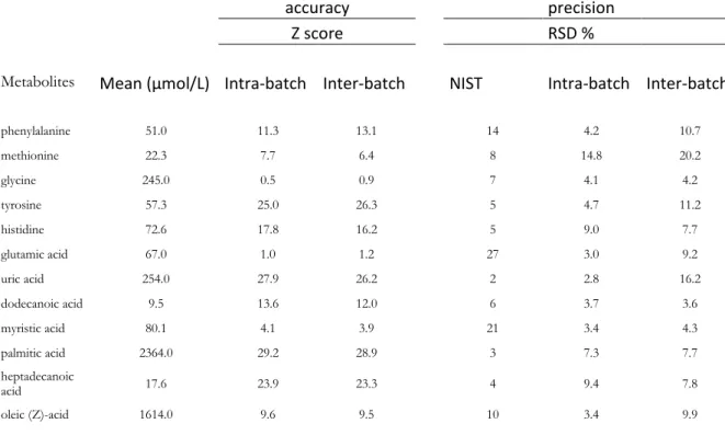
When necessary, it was completed by specific publications. Accuracy, Precision, and Recovery. The 2D peak volume accuracy compared, through z scores, the NIST certified or reference values of the 28 monitored metabolites to the corresponding measured values (corrected with the most chemically similar IS). As a result, the method was found to be limited to semiquantitation due to the lack of the exact response factors (Table 1 and Section S7 of the Supporting information Information). However, for glycine, the only NIST metabolite that we used as an IS, the response factor was calculable and the z scores were <1 in both intra- and inter-batch evaluations (0.5 and 0.9, respectively). Therefore, absolute quantitation seems possible but at the cost of one IS per compound with proper calibration, which would be extremely difficult to achieve in global profiling.11
The precision was assessed through the relative standard deviation in intra- and inter-batch measurements. The chromatographic separation was found to be stable and reproducible regarding the retention times, measured in the QC samples (Supporting Information, Section S4). Regarding the peak volumes, the RSD measured in the NIST samples was under 30% for all 28 metabolites monitored in both intra- and inter-batch evaluations. They were even under 10% for 24 and 18 metabolites. This is comparable to the NIST reported values,87 in fact, lower in 13
and 7 cases. It shows the stability of the method that could nevertheless be further improved through the automation of the sample preparation. In the QC samples, the peak volume precision was lower, albeit still good, with 14 and 11 metabolites (out of 16 since the IS had no variation after normalization), having an RSD < 30%. GC−MS data reported previously88 found RSD values lower than 20% for all the 32 representative compounds tested and lower than 10% for most of them. The modulation system and the second chromatographic column therefore seem to be a source of additional variations, hence the need to correct and monitor the peak volumes, here through the use of a QC system and LOESS (partial) correction. It is particularly true for multiple batches since the precision was lower in inter-batch measurements. Homogenization issues due to manual aliquoting could explain the higher RSD in the QC samples compared to the NIST SRM, although the metabolites monitored were not the same. Such issues have been
reported.88 It is of primary importance since the QC samples constitute the core of the global
quality system on which the method relies. In addition, they should also be aliquots of all the study samples, which is a minor limitation of this study.
Regarding the recovery, the differences between the response factors of the standards73
prevented the direct comparison of their signals, especially between the non-derivatized injection standard and the others, which is why negative recoveries were obtained in this case. If absolute values cannot be interpreted, their reproducibility is still meaningful.89 We found a
maximum RSD of 15.6% for three different batches of SRM 1950 and QC samples (Supporting Information, Section S8), indicating the robustness of the optimized sample preparation.
Linearity, Range, and Sensitivity. These parameters were evaluated using glycine-2,2-d2, succinic acid-2,2,3,3-d4, and fumaric acid-2,3-d2 added to QC samples at five different concentrations (process blank17 and 0.05, 0.25, 1.67, and 10 μg/ mL), each in six replicates. Selective m/z values representative of the IS (deuterated masses) were chosen and used in different types of regressions of increased complexity (unweighted and √S, S, S2, S3, and S4 weights) in order to take the uncertainty of measure into account. To assess these regressions, we avoided the R2 coefficient and preferred the sum of relative errors, the residual plots,90 the
range of linearity, and the sensitivity. We found that using a weighted regression was more efficient for succinic and fumaric acids (S2 weights for both). However, the regression parameters of the second were only slightly changed (from y = 43,158x + 6964 to y = 44,021x + 9; see the Supporting Information, Section S9, for details). Glycine and fumaric acid were reproducibly linear along the whole range tested. Succinic acid showed distinct behaviors below and above 0.25 ng/μL. The one below was used to assess the sensitivity. The limits of detection and quantification (LOD, LOQ) were calculated using the regression curves,91 process blank17
samples,92−94 and the relative standard deviation (RSD) of real injections95 (Supporting
Information, Section S10A). As a result, fumaric and succinic acids had consistently low LODs (approximately 2 and 5 pg on the column, respectively) and LOQs (6−9 and 16 pg on the column; Supporting Information, Section S10B, for details). Glycine, due to its higher blank signal, had a respective LOD and LOQ of 64 and 90 pg on the column. This was in good agreement with previous GC×GC studies,80,95 especially the one from Koek13 who used an S/N method
(extrapolated S/N = 3) and various chromatographic columns settings and obtained LODs ranging from 0.5 to 4 pg on the column for fumaric and succinic acids and from 70 to 280 pg for glutamine (glycine was not assessed). Our results were also compared advantageously with GC−MS where a method optimized for extraction and derivatization reported an LOD of approximately 1−5 pmol on the column88 (100−500 pg injected on the column for an average molecular mass of 100 g/mol and 1 μL injection). In addition, we manually controlled the selectivity through the chromatographic and mass spectral resolutions of the metabolites, which was facilitated by the 2D chromatogram visualization offered by GC×GC. The stability of the derivatized compounds was maximized by limiting the storage time before injection to 2 h at −20 °C.18,27 Overall, despite the impossibility to reach optimal conditions for all metabolites,11 the method was found to be fit-for-purpose. Indeed, according to the results obtained for the metabolites assessed, it should allow the untargeted sensitive detection and semiquantitation (linear behavior) of a large range of metabolites of various chemical classes and concentrations in a stable, therefore reproducible, manner. To do so, the ISs have to be representative of the many metabolites present in the samples. Therefore, the method presented could be further
improved by using a larger pool of (carefully selected) ISs. We would recommend to inject at least three ISs per major chemical class and one per minor one. One IS per intensity level (high, medium, or low) and one per retention window (1tR divided into three equal parts). One could also find it useful to implement some recently developed procedures that combine various ISs (CCMN96 and NOMIS97). Absolute quantification, which would require one IS per compound, seems out of reach for global profiling in the actual state of the field. Finally, the method developed for the untargeted analysis of 30 μL of serum samples should be adaptable to other matrices common in metabolomics, such as plasma and urine.37,50 QC System. A QC system repeats QC sample injections to monitor the stability of the performances over time, providing assurance of the quality16 of the data. It can also be used to increase it by correcting for the
analytical variations through an LOESS procedure.23 Here, control charts were constructed for
the 19 representative compounds defined at the validation step. Based on the validation results as well as on previous studies,80,57 the acceptable variations (around the mean value) for the retention times in both dimensions and normalized peak volumes were set to 2 times the modulation period, 5% of the PM, and 30% of the mean. The warning and action limits were drawn at 2 and 3 times these values. Finally, acceptance and rejection criteria were defined for individual injections and batches (Supporting Information, Section S11A). The resulting charts confirmed that the retention times and therefore the chromatographic separation were very stable. Indeed, 18 representative metabolites were well inside the warning limits. The only exception was the cysteine 1tR. Regarding the peak volumes, 11 and 1 metabolites (out of 16 since the 3 ISs were completely corrected by the normalization) had all their nine values inside the warning and action limits. For the four metabolites remaining, which violated at least once the action limits, the control charts were reconstructed with warning and action thresholds set to 2 and 3 times their measured standard deviations.98 This way, the system was considered
under control as long as these metabolites behaved within their usual ranges of values, even if it was over the acceptable 30% threshold. From a methodological point of view, the results obtained with nine injections over two days seemed to define well enough the control state of the analytical system. Anyway, for studies analyzing large cohorts over long periods of time, it would be advisable to inject multiple batches (at least five) of multiple (at least three) daily samples distributed over at least two weeks. Performing maintenance actions in that time frame would allow to evaluate their influence on the system. A representative example of a QC chart is provided in Figure 1.
Table 1. Intra- and Inter-Batch Accuracy and Precision Values for Selected Metabolites Assessed in the NIST SRM 1950
accuracy precision
Z score RSD %
Metabolites Mean (μmol/L) Intra-batch Inter-batch NIST Intra-batch Inter-batch
phenylalanine 51.0 11.3 13.1 14 4.2 10.7 methionine 22.3 7.7 6.4 8 14.8 20.2 glycine 245.0 0.5 0.9 7 4.1 4.2 tyrosine 57.3 25.0 26.3 5 4.7 11.2 histidine 72.6 17.8 16.2 5 9.0 7.7 glutamic acid 67.0 1.0 1.2 27 3.0 9.2 uric acid 254.0 27.9 26.2 2 2.8 16.2 dodecanoic acid 9.5 13.6 12.0 6 3.7 3.6 myristic acid 80.1 4.1 3.9 21 3.4 4.3 palmitic acid 2364.0 29.2 28.9 3 7.3 7.7 heptadecanoic acid 17.6 23.9 23.3 4 9.4 7.8 oleic (Z)-acid 1614.0 9.6 9.5 10 3.4 9.9
Figure 1. Control chart of the peak volume (normalized raw signal against time of analysis in days) of glutamic acid. All values lie inside the action limits (bold dashed lines, μ ± 3σ/√n). The ones lying outside the warning limits (light dashed lines, μ ± 2σ/√n), that is, days 1, 7, and 14, could indicate some analytical instability, which would have to be confirmed on the other monitored metabolites.
To further evaluate the analytical platform developed as well as to design and assess proper workflows for data (pre)processing, statistical treatments, bias control, and performance assessment (summarized in Figure 2), a real-life biomarker research study was conducted. It aimed to separate the Crohn’s disease samples put together regardless of the endoscopic activity (n = 35) from the healthy controls (n = 33). Further, the possibility to separate the three subgroups of Crohn’s disease patients from each other was evaluated. Raw Data Processing. A total of 922 unique peaks were consistently detected across all the study chromatograms of which 524 were kept after manual control for their chromatographic and mass spectral specificity. This is in good agreement with the 517 and 566 peaks obtained by Almstetter99 and
Castillo,80 respectively, and empirically confirms the high peak capacity of this analytical
platform. Further preprocessing included an LOESS (partial) correction and selection (Figure 2), which effect is shown in the Supporting Information, Section S11B. It led to a final data set of 183 metabolites having an RSD of <30%, almost twice as many as with 1D GC−MS,57 despite the
strict quality criteria applied. This demonstrates the added value of comprehensive GC×GC in untargeted applications. The exact chemical nature of the additionally resolved and detected metabolites was not investigated. Most probably, they belonged to the classes usually seen in GC−MS, that is, mainly amino acids, organic/carboxylic acids, fatty acids, sugars, and sugar alcohols.55,57 The selection made not only aimed to guarantee the quality of the data but also
reduced the size of the data set and made it easier to handle at the following steps. Data Scaling. We tested the effect of auto, pareto, level, range, and vast scaling on the structure of the data-natural trends and outliers-and on the biomarker research,21,100 here to separate the four groups
of samples at once. To do so, we applied unsupervised hierarchical clustering analysis (HCA) and principal component analysis (PCA) along with the 95% confidence ellipse.101 We also selected
various, differently operating, supervised methods: univariate ones: analysis of variance (ANOVA), Fisher ratios, and Stepdisc feature selection and multivariate ones: partial least squares discriminant analysis (PLS-DA) and random forests (RF). We found that level scaling was very sensitive to minor differences in samples. It tended to artificially create outliers that did not seem to exist in the raw data and was left out (see the Supporting Information, Section S12, for related figures). The other four methods produced similar PCA and PLS-DA plots as well as RF results. All had a positive effect on biomarker research in comparison to the raw data and led to the same selection of metabolites with similar significance values. Auto and range were slightly better in prediction with the highest predictive Q2 (0.28 and 0.31, respectively, on the whole dataset), in accordance with results from van den Berg et al.21 However pareto was
chosen because it maintained more of the initial structure (PCA and HCA) and was reported to be more stable than these two methods.21 In summary, at the exception of level scaling, the
methods tested here, based on mean centering, acted positively and similarly on the data structure and biomarker research, confirming that data scaling can affect the final results21 and
should be considered in method development. Overall, the proposed raw data processing workflow maintained the integrity of the data while preparing them for the following statistical treatment. Biomarker Research. In recent years, several protocols of high quality have been published, which aimed to standardize the main steps of a metabolomics analysis, including data preprocessing and processing.23,73,101 Indeed, standardization seems to be the next step in the
field.17 The protocols for biomarker research voluntarily limit the process to several successful
methods, such as RF, ANOVA, receiver operating characteristic (ROC) curves, and bootstrap validation. Nevertheless, other methods exist, and even the advocates of standardization
recognize that no workflow is appropriate in all situations.101 For this reason, in the
experimental procedure presented here, the data set was submitted to multiple tests characterized by different ways of operating algorithms and assumptions,101 such as correlation
versus hypothesis testing versus modelization versus diagnosis and parametric versus non parametric methods. By doing so, we intended to obtain a comprehensive and robust process applicable on data sets of various structures and sizes, including the ones characterized by low subject-to-variable ratios. However, in order to not complicate it excessively, a prior selection of the methods used was made based on general statistical knowledge and literature review. Practically, the first step consisted of the application of univariate testing (Fisher ratios (FR), correlations, and ANOVA; the exact test depending on the normality of the distribution), multivariate feature selection (Stepdisc, Runs, and Relief filterings), and multivariate modelization (orthogonal partial least-squares discriminant analysis (OPLS-DA), PLS-DA, RF, Naive Bayes classification, support vector machine (SVM), and neural networks (NN)). Individual fold changes (FC), two- tailed statistical power (through Cohen’s d102,103), and ROC
curves were also determined. Further details are given in the Supporting Information, Section S13A. Second, multiple testing and overfitting issues were taken into account through Bonferroni correction for univariate analysis104 and resampling error rates (bootstrapping,
cross, and leave-one-out validations) for multivariate analysis, respectively.101 Third, the
metabolites were ranked according to their significance based on p values, order of selection, weight, or variable importance in the projection (VIP) score. The most consistently significant ones were selected as candidate biomarkers (CB; Supporting Information, Section S13B).101,105
Fourth, to reduce the chance of missing any discriminant compound,104 the candidates were
removed from the data set and PLS-DA, OPLS-DA, and RF were applied to it. In the same perspective, we compared the supervised plots drawn on the data set before and after the selection and removal of the candidates. Again, the procedure is summarized in Figure 2. Its application to discrimination between the Crohn’s disease samples and healthy controls gave slight differences between the techniques, especially for Bayes classifier, neural networks,106 and
SVM.22 Apart from that, the same candidates were consistently highlighted as the most significant ones (n = 22) (Table 2 and Section S14 in the Supporting Information for detailed results). The discrimination between the three Crohn’s disease subgroups, characterized by different endoscopic activities, suffered from the nonapplicability of ROC curves, OPLS-DA, SVM, FC, and statistical power (number of classes > 2) as well as from the difficulty to interpret the Bayes classifier and neural network in terms of variable importance in such a case (Section S15). In addition, the statistical values obtained were lower than for the comparison between the CD and healthy control (HC) samples. Three reasons could contribute to explaining this: first, the logically higher biological proximity of the samples, second, the limits of the analytical method with the metabolites detected with this technique in this matrix possibly not being able to fully discriminate, and third, the difficulty for the statistical methods and models to differentiate three groups at once. It could justify the restratification of the data set to test new binary and therefore simpler hypotheses of work. This would also increase the number of possible methods available and facilitate the interpretation in terms of explanatory variables.101 Despite this issue,
29 candidates were consistently highlighted. Twelve of these were common to the previous separation and could be of particular interest in biological interpretation if confirmed on another cohort of patients. In both cases, the PLS-DA/OPLS- DA/RF posterior tests did not highlight any new potential candidate. In addition, the comparison of the supervised plots before
and after the removal of the candidates showed a large degradation of the separation, which supported the efficiency of the selection process. Based on these results, we consider that, for the global profiling of complex samples, the most appropriate methods are correlations (both Pearson/Spearman and Kendall), FC, Welch, or Kruskall-Wallis ANOVA or Fisher ratios (all working on a F distribution), Stepdisc as feature selection, PLS-DA and RF as modeling methods, ROC curves, univariate statistical power, and boxplots. Here, these methods managed well the small sample sizes (minimal n = 9), the noise inherent to biological variables, and, for the multivariate ones, the many variables encountered. If using all of them takes time and demands efforts, it gives a more comprehensive view of the data set. At least two or three should be used to be able to cope with any malfunctioning. Regarding the other techniques, they do not seem absolutely necessary because they are not always applicable (neither are ROC curves and statistical power); they can be more difficult to interpret (weights) and/or they tend to be redundant. Indeed, here, the same candidates were selected whether they were used or not (Table S15). Nonetheless, these methods can be useful in specific cases if satisfying results cannot be found otherwise. In general, the consensus metabolites are the most reliable and should be selected first as candidates. The significant compounds highlighted by only one or a few methods should be further investigated by looking to the raw data (FC, boxplots, presence of atypical values that could alter the parametric methods, and influence of zero values or ties). Looking for possibly missed interesting metabolites is also useful, particularly since the number and significance of the candidates depend on the biological proximity of the groups as well as on the coverage of the metabolome allowed by the analytical instrumentation. Finally, since it is difficult to define precisely what is a relevant feature,101 one could find it desirable to adapt the
selection thresholds. For example, it seems acceptable in an exploratory perspective to overlook the Bonferroni correction, provided that it is mentioned. It is however not advisable to lower them too much. Bias Control. Despite careful experimental design and selection of the samples, confounding factors can have a non- negligible105 impact to the point that they could be the
“most important threat to validity”.107 The following procedure was designed to avoid spurious
results104,16 by assessing the extent to which the candidate biomarkers truly reflected the classes
of interest and not the bias factors. All metadata available were considered: analytical: injection order, hemolysis of the samples, sample extraction, and drying, and clinical: age, gender, body mass index (BMI), disease location, tobacco and alcohol consumptions, medication for hypothyroidism, gastroesophageal reflux and ulcers, antitumor necrosis factor α (anti-TNFα), and immunosuppression (Section S1). The statistical methods employed were chosen to deal with the various situations met. First, the repartition of the factors between the biological classes studied was investigated:104 for continuous variables, through Pearson’s r or Spearman’s
ρ, according to normality, as well as Kendall’s τ, Welch ANOVA, and Kruskal-Wallis test and, for categorical ones, through, Goodman-Kruskal’s τ, and Theil’s U. As a complement, the means, medians, and percentages were compared between the classes, and boxplots and scatterplots were drawn. When a factor was not adequately matched between the groups, we aimed to determine which candidates it could affect. The second step therefore evaluated the direct relationship between the factor and the candidates. Through Pearson’s r or Spearman’s ρ, according to normality, as well as Kendall’s τ, Welch ANOVA, and Kruskal-Wallis test. Third, we looked for the effect of the factor on the candidates’ ability to discriminate, the very point of the study. It was done through partial correlations and the equilibration of the classes for the confounding factor. To do the latter, we determined the samples most responsible for the
imbalance and we temporarily removed them. After which, the new repartition was tested again for imbalance. Then, correlations (Pearson/Spearman and Kendall), Welch ANOVA and Kruskal-Wallis tests, individual fold changes, and ROC curves were compared before and after the removal, that is, with and without the imbalance. As a visualization tool, PCA101 and HCA plots
were constructed on the candidates with each point tagged according to the bias factor. For categorical bias factors having a sufficiently low number of subgroups, boxplots and univariate ROC curves were drawn according to those subgroups and compared. The global protocol is summarized in Figure 2. Regarding the separation between the CD samples and the HC, the anti-TNFα and immunosuppressive medications had significant imbalance (p values of <0.01 and <0.05, respectively, see the Supporting Information, Section S16). Nine and twelve candidates were found to be linked to the two factors at various degrees, but only three of them were biased to such an extent in that their residual ability was too poor to still be significant. They were therefore removed from the set of biomarkers. In the separation between the CD subgroups, unequal repartitions were observed for the anti-TNFα (p value of <0.01) and immunosuppressive medications as well as for the age and BMI of the patients (p values < 0.05, Supporting Information, Section S17). Five, four, seven, and three candidates were correlated to these factors. The control of the residual ability to separate relied only on the equilibration because of the unavailability of partial correlations for K > 2. It led to the removal of five candidates. Two others were biased but still discriminant. They were therefore not taken into account in the separation performance assessment but kept as relevant metabolites. To conclude, the procedure proposed dealt well with both continuous and categorical factors, both normal and non-normal distributions, and small sample sizes. It appeared to be efficient as well as suitable for the bias factors and the data structure that we were confronted with. It remained quite simple despite the complexity inherent to such a process.107 It should therefore be
applicable and beneficial to other studies willing to control for potential biases. Three more things should be noted regarding the practical use of this procedure. First, it aims less to reject candidate biomarkers, even if it can be used to do so, than to evaluate and document their reliability. This is of primary importance, for example, for meta- analysis. Second, the process is sensitive to the sample size. Large cohorts are helpful to smooth the data relative to potential bias factors as well as to keep enough patients after the equilibration to maintain statistical significance. Third, the procedure can only control the presence of potential known biases, not correct for them. Therefore, it does not replace in any way an appropriate experimental design where the samples are matched as properly as possible, given the usual clinical limitations. Classification and Separation Performances of the Candidate Biomarkers. The goal here was to see if the statistically significant associations measured could lead to biomarkers able to discriminate.16 First, the unbiased candidates highlighted for both separations (n = 19 and n =
22) were sequentially grouped, starting with the most discriminant ones, into metamarkers (Supporting Information, Section S18A). Second, their performances were assessed, again with multiple methods:101 separation space visualization: HCA, PCA, PLS- DA, and OPLS-DA plots; PLS-DA and OPLS-DA classification models; linear discriminant analysis (LDA): Hotelling’s T2 and Wilks’s λ through Rao transformation, the most appropriate for small sample sizes;108
multivariate ROC curves using several algorithms; multivariate statistical power; and mean error rates for LDA, Bayes classifier, PLS-DA, neural network, and SVM models. When applicable (classification models, error rate models, and ROC curves), permutation testing and resampling (including bootstrapping)101 and test validations were also evaluated.104 For the latter, training
and test sets were constructed in a 2:1 ratio,104 and they were matched and tested for biases
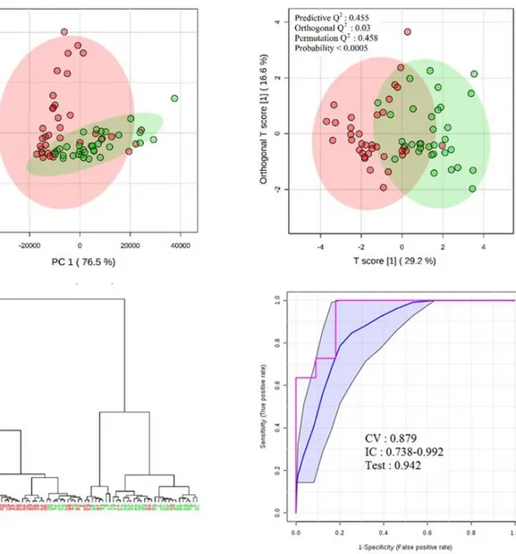
(Supporting Information, Section S18B). Third, to further assess the relative significance of the candidates, we considered their respective order of importance in the performance models. A summary of this protocol can be found in Figure 2. The results showed that the CD samples were effectively and consistently separated from the HC. The diagnosis ability (ROC) was also good104,109 with the most efficient model able to diagnose with 100% sensitivity and 82%
specificity (Figure 3 and Section S19 in the Supporting Information for the detailed results). For a given method, the performances were similar regardless of the number of candidates included in the meta-marker. This means that the most significant candidates, which formed the core of all the metamarkers tested, produced most of the separation and therefore should be used in classification.104 In the meantime, the three CD subgroups could not be completely separated,
and the performances were logically lower (Figure 4 and Section S20 in the Supporting Information). Among the three possible reasons for this, already exposed in Biomarker Research, the most influential here is the difficulty to discriminate more than two classes with only one frontier of separation,101 regardless of the sophistication of the algorithm. Indeed, it
makes it harder for the models to deal with the inherent noise of the variables and to distinguish it from the biologically interesting information. It thus decreases the performances and makes it necessary to employ more variables to achieve sufficient separation. Another issue already mentioned is the nonapplicability of ROC curves, OPLS-DA, SVM, and statistical power for more than two classes. In both cases, the various models converged,101 and the candidates selected as
the most significant were found to be the most influential in the performance models. In addition, when the QC samples were added to the plots, they were grouped at the center, close to the healthy controls. This indicated that the analytical variability was much lower than the biological one and confirmed the stability of the designed analytical process.16 From a
methodological point of view, using methods that operate differently allows a comprehensive assessment of the candidates, that is, a broad perspective on their separation, classification, and potential diagnosis capabilities. We particularly recommend to employ an OPLS-DA model, LDA model, error rates for PLS-DA, ROC curves (RF algorithm), and PCA, HCA, and OPLS-DA plots. Resampling and test validations as well as permutation testing should be used because they evaluate more accurately the generalization of the models to new samples. They also allow the calculation of confidence intervals, both features that are particularly important with low sample sizes. The order of importance of the candidates in the classification models (particularly PLS-DA, OPLS-DA, and RF) is a useful evaluation of their relative effectiveness. Adding the QC samples to the unsupervised PCA and HCA plots is a useful posterior control of the analytical quality of the data. To finish, it is important to stress that, regardless of their usefulness in prediction, all candidate biomarkers and, more largely, all significantly altered metabolites have a potential biological interest and should be kept, provided that they are reliably identified or at least annotated. Annotation of the Candidate Biomarkers. Of the 33 unique, unbiased candidates, 10 met the three defined mass criteria and 7 met two of those (Table 3; all metabolites are given in the Supporting Information, Section S21). Two of them, terephthalic acid and threonolactone, were not reported to have any biological function and were probable artifacts (see the Supporting Information, Section S22). Terephthalic acid is a bulk chemical used to produce polyethylene terephthalate (PET). It was likely introduced by a plastic material used in the analytical process, such as gloves, despite the subtraction of the process blank in the data preprocessing. Threonolactone is a biological artifact produced by the autoxidation of L-ascorbic
acid in methanol,110 the solvent used here for protein extraction. For this reason, it has been
found to have poor chemical stability in urine.111 By combining three kinds of information,
putative (Metabolomics Standards Initiative (MSI) level 2) annotations112,113,23 were achieved for
approximately half of the candidates. Such a typical fraction28 is quite satisfactory given the
complexity of the metabolome. On the other hand, it means that half of the significant metabolites are lost for any clinical or biological use.109 Increasing the resolution from 5000 to
25,000 (mass error from 3−100 ppm to 1 ppm or less) and using linear retention indices improved the confidence of the annotation. It also compensated for the lack of specificity of the low-resolution mass spectra due to the derivatization masses (m/z 73 and 147). In addition, LRIs were confirmed114 to be particularly useful for sugars because of their unselective mass
spectra and the absence of the molecular ion in electron ionization (EI). Using a pool of alkanes limited to C20 was found to be sufficient, given that the indices were extrapolated over C20 (linear temperature ramp). Importantly, any method willing to achieve non equivoque, level 1 identification, should compare the mass and retention information measured to the ones of the corresponding standards analyzed on the same platform under the same conditions.112,113,23 The
literature review that included various biological matrices and various analytical platforms showed that, among the annotated candidates, several had previously been associated to and are therefore likely to play a role in CD, IBD, and, more largely, gastrointestinal inflammation processes (Supporting Information, Section S23). It also showed that there is little consensus about the candidate biomarkers, sometimes even for similar matrices studied with similar instrumentations. In agreement with Barding,55 the candidates highlighted with NMR (and
obviously GC-MS) belong to chemical classes observable with GC×GC. Therefore, while this is not the goal of this untargeted study, this instrumentation is capable of targeting and challenging most of the significant metabolites found in other studies with the exception of the more lipidic fractions observed with LC−MS. In addition, due to its increased sensitivity and resolution, it is able to detect more metabolites, that is, more potential candidates, including new ones.
Figure 2. Summary of the global data processing workflow from raw data to verified and annotated candidate biomarkers.
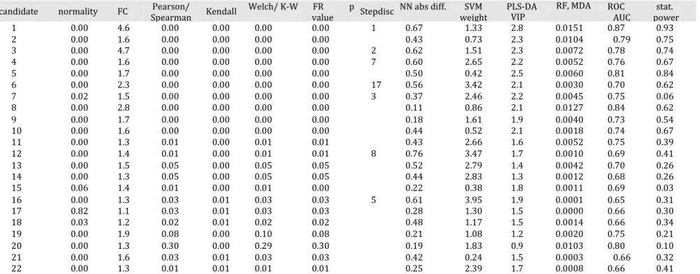
Table 2. Main Statistical Values for the Candidate Biomarkers Able to Discriminate the CD Samples from the Healthy Controlsa candidate normality FC Pearson/
Spearman Kendall Welch/ K-W FR p value Stepdisc NN abs diff. SVM weight PLS-DA VIP RF, MDA ROC AUC stat. power 1 0.00 4.6 0.00 0.00 0.00 0.00 1 0.67 1.33 2.8 0.0151 0.87 0.93 2 0.00 1.6 0.00 0.00 0.00 0.00 0.43 0.73 2.3 0.0104 0.79 0.75 3 0.00 4.7 0.00 0.00 0.00 0.00 2 0.62 1.51 2.3 0.0072 0.78 0.74 4 0.00 1.6 0.00 0.00 0.00 0.00 7 0.60 2.65 2.2 0.0052 0.76 0.67 5 0.00 1.7 0.00 0.00 0.00 0.00 0.50 0.42 2.5 0.0060 0.81 0.84 6 0.00 2.3 0.00 0.00 0.00 0.00 17 0.56 3.42 2.1 0.0030 0.70 0.62 7 0.02 1.5 0.00 0.00 0.00 0.00 3 0.37 2.46 2.2 0.0045 0.75 0.06 8 0.00 2.8 0.00 0.00 0.00 0.00 0.11 0.86 2.1 0.0127 0.84 0.62 9 0.00 1.7 0.00 0.00 0.00 0.00 0.18 1.61 1.9 0.0040 0.73 0.54 10 0.00 1.6 0.00 0.00 0.00 0.00 0.44 0.52 2.1 0.0018 0.74 0.67 11 0.00 1.3 0.01 0.00 0.01 0.01 0.43 2.66 1.6 0.0052 0.75 0.39 12 0.00 1.4 0.01 0.00 0.01 0.01 8 0.76 3.47 1.7 0.0010 0.69 0.41 13 0.00 1.5 0.05 0.00 0.05 0.05 0.52 2.79 1.4 0.0042 0.70 0.26 14 0.00 1.3 0.05 0.00 0.05 0.05 0.44 2.83 1.3 0.0012 0.68 0.26 15 0.06 1.4 0.01 0.00 0.01 0.00 0.22 0.38 1.8 0.0011 0.69 0.03 16 0.00 1.3 0.03 0.01 0.03 0.03 5 0.61 3.95 1.9 0.0001 0.65 0.31 17 0.82 1.1 0.03 0.01 0.03 0.03 0.28 1.30 1.5 0.0000 0.66 0.30 18 0.03 1.2 0.02 0.01 0.02 0.02 0.48 1.17 1.5 0.0014 0.66 0.34 19 0.00 1.9 0.08 0.00 0.10 0.08 0.21 1.08 1.2 0.0020 0.75 0.21 20 0.00 1.3 0.30 0.00 0.29 0.30 0.19 1.83 0.9 0.0103 0.80 0.10 21 0.00 1.6 0.03 0.01 0.03 0.03 0.42 0.24 1.5 0.0003 0.66 0.32 22 0.00 1.3 0.01 0.01 0.01 0.01 0.25 2.39 1.7 0.0008 0.66 0.41
a Univariate tests : FC, Pearson, Spearman, and Kendall correlations, Welch and Kruskal-Wallis (K-W) tests, FR, and statistical power. Multivariate methods: Stepdisc feature selection, NN (absolute distance between the groups), PLS-DA, and RF (mean decrease accuracy). Diagnosis: ROC (area under the curve, AUC). The values meeting the statistical thresholds set for significance are in bold.
Figure 3. HCA and PCA plots (six candidates used), OPLS-DA plot (12 candidates), and ROC curve (all 19 candidates, RF algorithm) for the separation between the CD samples (red) and the HC (green). In the ROC curve, the blue line pictures the mean value of the 100 cross validation classifications, the blue surface represents the corresponding confidence intervals at 95%, and the red line pictures the test classification.
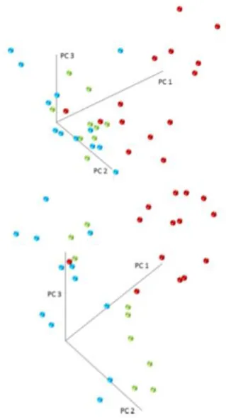
Figure 4. 3D PCA plot (top, six candidates used; PC1: 80.2%, PC2: 8.7%, and PC3: 5.5%) and PLS-DA plot (bottom, 22 candidates used; PC1: 30.5%, PC2: 19.8%, PC3: 9.3%) for the separation between the three CD groups. High-endoscopic activity samples are in red; low- endoscopic activity samples are in green and quiescent samples in blue.
aCandidates highlighted in the CD vs HC separation (top) and candidates highlighted in the three CD subgroups
separation (bottom). The values that meet the significance thresholds are in bold. *Threonolactone and terephthalic acid are probable artifacts.
CONCLUSIONS
This work showed that it is not straightforward to perform exploratory hypothesis-generating analysis on complex biological samples in a semiquantitative and reliable manner, particularly with a comprehensive analytical platform such as GC×GC−MS despite its power in terms of peak capacity. Indeed, if the global approach proposed was validated and successfully applied to separate Crohn’s disease samples from negative, “healthy” controls, it required careful optimization, the control and articulation of the various steps, the use of multiple statistical treatments and the evaluation of the potential biases that were not compensated in the experimental design. Regarding the results obtained, this study is limited to a proof of concept. Therefore, the candidates highlighted, despite their analytical and statistical reliability, cannot be seen as true biomarkers. To achieve that, the first step would be to perform a targeted quantitative analysis of the samples. Then, assuming that the variations observed would be confirmed, these compounds should be validated on a second independent set of samples to see if they translate to a different group of patients.
ASSOCIATED CONTENT
SUPPORTING INFORMATION
The Supporting Information is available free of charge at
https://pubs.acs.org/doi/10.1021/acs.jproteome.9b00535.
Sample collection and clinical and analytical metadata for the Crohn’s disease study (Section S1): clinical metadata for the samples of the proof of concept study (Table S1); security precautions for the sample preparation (Section S2); Box−Behnken design of experiment (Section S3); list of the metabolites monitored in the internal QC samples, intra- and inter-batch variations(Section S4): list of the 19 representative metabolites monitored in the internal QC samples (Table S2); list of the metabolites assessed in the NIST SRM 1950 (Section S5): extracts from the NIST SRM 1950 (metabolites in frozen human plasma) certificate (Figure S1); method optimization, sample preparation and separation and detection (Section S-6): DoE response surfaces for MSTFA and MeOX volumes and temperatures (Figure S2), sample preparation optimization (Table S3), examples of chromatograms produced by the three sets of columns (Figure S3), separation parameters for various flow rates and temperature ramps (Figure S4), chromatograms obtained at 3 and 5 °C/min (Figure S5), run times for the four temperature ramps evaluated (Table S4), effect of the initial temperature on the early eluting compounds (Figure S6), effect of the hot jet duration on the resolution in the overloaded zones of urea and glucose (Figure S7), influence of the injection temperature on the normalized peak volume (Table S5), impact of the injection volume on the chromatographic resolution in an area at risk of overloading (urea) (Figure S8), effect of the liner design on the global chromatogram (Figure S9), and summary of the optimized analytical conditions (Figure S10); accuracy and precision assessment in the NIST SRM 1950 (Section S7): accuracy and precision assessment in NIST SRM 1950 (Table S6); recovery assessment in the NIST SRM 1950 and the internal QC samples (Section S8): recovery assessment in NIST SRM 1950 and internal QC (Table S7); regression methods and determination of the best fit (Section S9): determination of the most efficient regression for succinic acid (Table S8), determination of the most efficient regression for fumaric acid (Table S9), determination of the most efficient regression for glycine (Table S10), residual plots for the three IS using unweighted and weighted regressions (Figure S11), and unweighted and weighted linear regression for succinic acid, fumaric acid, and glycine (Figure S12); sensitivity assessment, methods and calculation of LOD and LOQ (Section S10): LOD, LOQ, and sensitivity assessment using three different methods (Table S11); QC system, acceptance/rejection criteria and effect of the QC correction (Section S11): effect of the LOESS (partial) correction on the QC sample signals for two metabolites of the final dataset (Figure S13) and QC and study samples signals before and after the LOESS (partial) correction (Figure S14); data scaling (Section S12): HCA plots for the various scaling methods (Figure S15), PCA 3D plots for the various scaling methods (Figure S16), PCA 2D plots for level scaling with all samples and without the two alleged outliers (Figure S17), PLS-DA 3D plots for the various scaling methods (Figure S18), effect of scaling on random forests’ (RF) ability to highlight the most significant metabolites (Table S12), PLS-DA Q2 and R2 for the various scaling methods (Table S13), and percentages of variation explained by the first two axes in PCA and PLS- DA