Topics in image reconstruction for high resolution positron emission tomography

(1)

UNIVERSITÉ DE SHERBROOKE

TOPICS

IN

IMAGE RECONSTRUCTION FOR

HIGH RESOLUTION POSITRON

EMISSION

TOMOGRAPHY

par

Vitali Selivanov

Département de Médecine nucléaire et de radiobiologie

Thèse présentée à la Faculté de médecine

en vue de l'obtention du grade de

philosophiae doctor (Ph.D.) en radiobiologie

Sherbrooke (Québec) Canada

2002

(2)

l+I

National library

of Canada Bibliothèque nationale du Canada Acquisitions and

Bibliographie Services Acquisitions et services bibliographiques

395 Wellington Street Ottawa ON K1A ON4 Canada

395, rue Wellington Ottawa ON K1A ON4 Canada

The author has granted a

non-exclusive licence allowing the

National Library of Canada to

reproduce, loan, distnbute or sell

copies of this thesis in microfonn,

paper or electronic formats.

The author retains ownership of the

copyright

in

this thesis. Neither the

thesis nor substantial extracts :from it

may be printed or otherwise

reproduced without the author' s

penmss10n.

Your file Vo"" référence

Our file Narre rélénmœ

L'auteur a accordé une licence non

exclusive permettant

à

la

Bibliothèque nationale du Canada de

reproduire, prêter, distribuer ou

vendre des copies de cette thèse sous

la

forme de microfiche/film, de

reproduction sur papier ou sur format

électronique.

L'auteur conserve

la

propriété du

droit d'auteur qui protège cette thèse.

Ni

la

thèse

ni

des extraits substantiels

de celle-ci ne doivent être imprimés

ou autrement reproduits sans son

autorisation.

0-612-80550-6

(3)

Abbreviations

1-D 2-D 3-D ART CLT CT CV DFM DRF ECT EM FBP FOY KL LOR MAP ML MLE ML-EM OS-EM PET PSF PWLS RAMLA ROI r.v. one-dimensional two-dimensional three-dimensional

algebraic reconstruction technique central limit theorem

computed (or computerised) tomography cross-validation

direct Fourier method detector response function emission computed tomography expectation maximisation filtered backprojection field-of-view Karhunen-Loève ( transform) line-of-response maximum a posteriori maximum likelihood

maximum likelihood estimate

maximum likelihood via expectation maximisation (algorithm)

(maximum likelihood via) expectation maximisation with ordered subsets (algorithm) positron emission tomography

point spread function

penalised weighted least-squares

row-action maximum likelihood algorithm region-of-interest

(7)

SNR SPECT SVD TAC TOR TSVD WLS signal-to-noise ratio

single photon emission computed tomography singular value decomposition

time-activity curve tube-of-response

truncated singular value decomposition weighted least-squares

(8)

List of Figures

FIGURE 1. SIMPLE CASE OF RADIOTRACER DISTRIBUTION AND TWO IDEALISED CONTINUOUS PROJECTIONS AT SELECTED ANGLES. . ... 6

FIGURE 2. FROM LEFT TO RIGHT: A) AN EXAMPLE OF THE SUPPORT REGION Q , WHICH IS THE ELLIPSE INTERIOR; B) ASETOFCONVENTIONALSQUAREPIXELS; C) ASETOFPOLARPIXELS ... 15

FIGURE 3. TUBE-OF-RESPONSE FOR A GIVEN DETECTOR PAIR ... 16

FIGURE 4. NATURAL PIXEL DEFINED AS AN INTERSECTION OF THE TUBE-OF-RESPONSE SHOWN IN THE

PREVIOUS FIGURE AND THE PET SCANNER FIELD-OF-VIEW ... 17

FIGURE 5. THE SINOGRAM OF AN OFF-CENTRE "POINT" SOURCE ... 18

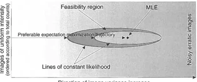
FIGURE 6. THE DIAGRAM SHOWING TWO ALTERNATIVE ROUTES THAT COULD BE TAKEN FOR AN APPROXIMA TE SOLUTION OF THE INVERSE PROBLEM ... 27

FIGURE 7. SCHEMATICS OF THE ML-EM IMAGE RECONSTRUCTION AND AN EXAMPLE OF THE FEASIBILITY

REGION ... 39

FIGURES APPEARING AS A PART OF THE FOLLOWING PUBLICATIONS (NOTE THAT THE REFERENCES TO OTHER FIGURES IN THE FOLLOWING CAPTIONS REFER TO SAME ARTICLE):

[4.1] SELIVANOV V V, PICARD Y, CADORETTE J, RODRIGUE S, AND LECOMTE R 2000

DETECTOR RESPONSE MODELS FOR ST ATISTICAL ITERATIVE IMAGE RECONSTRUCTION

INHIGHRESOLUTIONPET IEEE TRANS. NUCL. SC!. 471168-75

FIGURE 1. PHANTOMS USED TO ACQUIRE DATA WITH THE SHERBROOKE ANIMAL PET SCANNER ... .

54

(9)

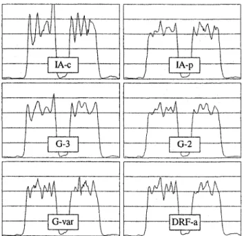
FIGURE 3. Two EXAMPLES OF SIX DIFFERENT DRF MODELS IN COMPARISON TO EXPERIMENTAL DRF ... 56

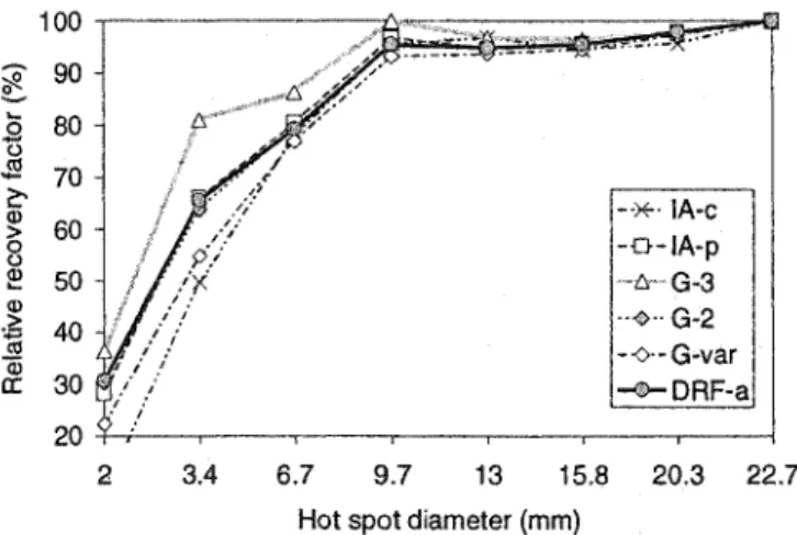
FIGURE 4. RESOLUTION PHANTOM RECONSTRUCTED USING SIX DIFFERENT DRF APPROXIMATIONS AND THE CROSS-VALIDATION PROCEDURE (FIRST RECONSTRUCTION SERIES) ... 58 FIGURE 5. PROFILES OF THE RESOLUTION PHANTOM (FIRSTRECONSTRUCTION SERIES) ... 58 FIGURE 6. CONTRAST PHANTOM RECONSTRUCTED USING SIX DIFFERENT DRF APPROXIMATIONS AND THE CROSS-VALIDATION PROCEDURE (FIRST RECONSTRUCTION SERIES) ... 58 FIGURE 7. PROFILES OF THE CONTRAST PHANTOM ILLUSTRATING THE EDGE ARTEFACT (FIRST RECONSTRUCTION SERIES) ... 58 FIGURE 8. RELATIVE RECOVERY FACTOR AS A FONCTION OF HOT SPOT SIZE, CALCULATED FROM THE CONTRAST PHANTOM IMAGES RECONSTRUCTED USING SIX DIFFERENT DRF MODELS (FIRST

RECONSTRUCTION SERIES) ... 59 FIGURE 9. RELATIVE STANDARD DEVIATION AS A FONCTION OF HOT SPOT SIZE CALCULATED FROM THE CONTRAST PHANTOM IMAGES RECONSTRUCTED USING SIX DIFFERENT DRF MODELS (FIRST

RECONSTRUCTION SERIES) ... .59 FIGURE 10. RELATIVE STANDARD DEVIATION WITHIN THE LARGEST HOT REGION OF THE CONTRAST PHANTOM AS A FONCTION OF ITERATION NUMBER (SECOND RECONSTRUCTION SERIES) ... .59 FIGURE 11. PROFILES OF THE CONTRAST PHANTOM ILLUSTRATING THE EDGE ARTEFACT (SECOND RECONSTRUCTION SERIES) ... 59 FIGURE 12. RELATIVE RECOVERY FACTOR AS A FONCTION OF HOT SPOT SIZE CALCULATED FROM THE CONTRAST PHANTOM IMAGES RECONSTRUCTED USING SIX DIFFERENT DRF MODELS (SECOND

RECONSTRUCTION SERIES) ... 60

FIGURE 13. RELATIVE STANDARD DEVIATION AS A FONCTION OF HOT SPOT SIZE CALCULATED FROM THE CONTRAST PHANTOM IMAGES RECONSTRUCTED USING SIX DIFFERENT DRF MODELS (SECOND

(10)

[4.2] SELIVANOV V V, LAPOINTE D, BENTOURKIA M, AND LECOMTE R 2001 CROSS-V ALIDATION STOPPING RULE FOR ML-EM RECONSTRUCTION OF DYNAMIC PET SERIES:

EFFECT ON IMAGE QUALITY AND QUANTITATIVE ACCURACY IEEE TRANS. NUCL. SC!. 48

883-9

FIGURE l. PHANTOM MODELING THE LEFf VENTRICLE OF A RAT HEART WAS USED TO ACQUIRE DATA FOR ASSESSING QUANTITATIVE ACCURACY OF DIFFERENT RECONSTRUCTION PROTOCOLS ... 64 FIGURE 2. NUMBER OF ML-EM ITERATJONS, DEFINED BY THE AUTOMATIC CV PROCEDURE, AS A FONCTION OF THE TOTAL COUNTS IN PHANTOM PROJECTIONS ... 65 FIGURE 3. DECA Y CORRECTED COUNT RATE c, IN THE PHANTOM ROI AS A FUNCTION OF THE TOTAL COUNTS IN THE PROJECTION DA TA ... 66

FIGURE 4. RATIO OF c, FOR ML-EM WITH THE CROSS-VALIDATION TO c, FOR 200 ML-EM ITERATIONS ... 66

FIGURE 5. PHANTOM IMAGES CONTRASTAS A FONCTION OF THE TOTAL COUNTS IN THE PROJECTION DATA ... 66 FIGURE 6. DEPENDENCE OF THE NUMBER OF ML-EM ITERATIONS, DEFINED BY THE AUTOMATIC CV

PROCEDURE, ON THE TOTAL COUNTS FOR THE RAT SERIES (CV STOPPING POINT), FUNCTJON FITTED

TO THE CV STOPPING POINTS (CVF), AND THE FITTED FONCTION DERIVED FOR THE PHANTOM

(CVF FOR PHANTOM, GIVEN IN FIG.2 AS WELL) ... 66

FIGURE 7. SELECTED FRAMES FROM THE DYNAMIC RAT SCAN, RECONSTRUCTED WITH DIFFERENT

TECHNIQUES ... 67

FlGURE 8. EARL Y PART OF THE BLOOD POOL TIME-ACTIVITY CURVES ... 67 FIGURE 9. LATE PART OF THE BLOOD POOL TIME-ACTIVITY CURVES ... 68 FIGURE 10. RMRGLC ESTIMATES COMPUTED FOR MYOCARDIAL ROIS USING TACS OF THE BLOOD

(11)

[4.3] SELIVANOV V V AND LECOMTE R 2001 FAST PET IMAGE RECONSTRUCTION BASED ON SVD DECOMPOSITION OF THE SYSTEM MATRIXIEEE TRANS. NUCL. SC!. 48 761-7

FIGURE 1. SJNGULAR VALUE SPECTRA OF THE SYSTEM MATRIX FOR THE SHERBROOKE ANIMAL PET SCANNER AND THREE DIFFERENT IMAGE GRIDS ... 73

FIGURE 2. SAME AS FIG. 1 ON A LOG-LOG SCALE SHOWJNG THE EXISTENCE OF A "PLATEAU" OF

SJNGULAR VALUES AND AN ABRUPT DROP-OFF OF THE SPECTRUM TAIL RESPONSIBLE FOR THE

SEVERE ILL CONDITIONING OF THE RECONSTRUCTION INVERSE PROBLEM ... 73

FIGURE 3. RADIAL FWHM LOCAL RESOLUTION ESTIMATES OF A POINT SOURCE IN THE FOY CENTER,

RECONSTRUCTED WITH TSVD WITH VARYING TRUNCATION INDEX T, 96X96-PIXEL IMAGE ... 7 4 FIGURE 4. POINT SOURCE IN THE FOY CENTER RECONSTRUCTED WITH TSVD, 96x96 PIXEL IMAGE ... 74

FIGURE 5. FWHM RESOLUTION ESTIMATES (LOCAL AND GLOBAL), DERIVED USING POINT SOURCE

IMAGES RECONSTRUCTED WITH TSVD, T=l217, 96x96 PIXEL IMAGE ... 75

FIGURE 6. PHANTOM IMAGES RECONSTRUCTED WITH: A) FBP; B) ML-EM (100 ITERATIONS); C)

TSVD, MATCHING FBP (GLOBAL) RESOLUTION (T=950); D) TSVD, MATCHING GLOBAL

RECONSTRUCTED IMAGE RESOLUTION TO THE INTRINSIC SCANNER RESOLUTION IN THE FOY

CENTER (T=l217) ... 75

FIGURE 7. IMAGE PROFILES THROUGH THE TWO LARGEST HOLES OF THE PHANTOM ALONG THE LINE

SHOWN IN FIG. 6D. A) FBP; B) ML-EM, 100 ITERATIONS; C) TSVD, T=950; D) TSVD, T=1217 . ... 76

FIGURE 8. RECOVERY FACTORS CALCULATED USING RECONSTRUCTED PHANTOM IMAGES SHOWN IN FIG. 6 ... 76

[4.4] SELIVANOV V V AND LECOMTE R LIST-MODE PET IMAGE RECONSTRUCTION BASED ON REGULARIZED PSEUDO-INVERSE OF THE SYSTEM MATRIX TO BE SUBMITTED

(12)

FIGURE l. SCHEMATIC OF THE EVENT-BY-EVENT RECONSTRUCTION PROCESS USING THE REGULARIZED PSEUDO-INVERSE MA TRIX.

105

FIGURE 2. SEQUENCE OF PHANTOM IMAGES DEMONSTRATING THE USE OF THE INCREMENTAL TSVD RECONSTRUCTION FOR A SYSTEM HAVING A COMPLETE RING OF DETECTORS ... 106

FIGURE 3. SEQUENCE OF IMAGES DEMONSTRATING THE USE OF THE INCREMENTAL TSVD RECONSTRUCTION FOR ROTATING BANKS OF DETECTORS, AN INCOMPLETE RING, ACQUIRING DATA

AT ONE PROJECTION ANGLE AT A TIME ... 107 FIGURE 4. RADIAL PROFILES THROUGH THE EXPECTED STANDARD DEVIATION MAPS WITH THE TSVD

RECONSTRUCTION FOR THREE DIFFERENT TRUNCATION LEVELS AND THE IMAGE OF 64x64 PIXELS .

... 108

FIGURE 5. RADIAL PROFILES THROUGH THE EXPECTED STANDARD DEVIATION MAPS WITH THE TSVD RECONSTRUCTION FOR THREE DIFFERENT TRUNCATION LEVELS AND THE IMAGE OF 96x96 PIXELS .

(13)

List of Tables

TABLES APPEARING AS A PART OF THE FOLLOWING PUBLICATIONS:

[4.1] SELIVANOV V V, PICARD Y, CADORETTE J, RODRIGUE S, AND LECOMTE R 2000 DETECTOR RESPONSE MODELS FOR STATISTICAL ITERATIVE IMAGE RECONSTRUCTION IN HIGH RESOLUTION PET IEEE TRANS. NUCL. SC!. 47 1168-75

TABLE l. NOTATION USED IN THE P APER ... 55 TABLE 2. TRANSITION MATRIX SIZE (NON-ZERO ELEMENTS ONLY), MB ... ..

56

TABLE 3. NUMBER OF ITERA TI ONS SUGGESTED BY THE CROSS-VALIDATION STOPPING RULE ... 57

[4.2] SELIVANOV V V, LAPOINTE D, BENTOURKIA M, AND LECOMTE R 2001 CROSS-V ALIDATION STOPPING RULE FOR ML-EM RECONSTRUCTION OF DYNAMIC PET SERIES: EFFECT ON IMAGE QUALITY AND QUANTITATIVE ACCURACY IEEE TRANS. NUCL. SC!. 48 883-9

TABLE 1. NOTATION USED ... 64

[4.3] SELIVANOV V V AND LECOMTE R 2001 FAST PET IMAGE RECONSTRUCTION BASED ON SVD DECOMPOSITION OF THE SYSTEM MATRIX IEEE TRANS. NUCL. SC!. 48 761-7

TABLE I. TRUNCATION INDEX T BASED ON SPATIAL RESOLUTION ANALYSIS (USING GLOBAL RESOLUTION ESTIMATES) ... 74

[4.4] SELIVANOV V V AND LECOMTE R LIST-MODE PET IMAGE RECONSTRUCTION BASED ON REGULARIZED PSEUDO-INVERSE OF THE SYSTEM MATRIX TO BE SUBMJTTED

TABLE I. EXPECTED SIZE OF THE (REGULARIZED) PSEUDO-INVERSE MATRIX FOR VARIOUS SINOGRAM SIZE ... 110

(14)

Abstract

Ill-posed problems are a topic of an interdisciplinary interest arising in remote sensing and non-invasive imaging. However, there are issues crucial for successful application of the theory to a given imaging modality. Positron emission tomography (PET) is a non-invasive imaging technique that allows assessing biochemical processes taking place in an organism in vivo. PET is a valuable tool in investigation of normal human or animal physiology, diagnosing and staging cancer, heart and brain disorders. PET is similar to other tomographie imaging techniques in many ways, but to reach its full potential and to extract maximum information from projection data, PET has to use accurate, yet practical, image reconstruction algorithms. Several tapies related to PET image reconstruction have been explored in the present dissertation. The following contributions have been made:

~ A system matrix model has been developed using an analytic detector response

fonction based on linear attenuation of y-rays in a detector array. It has been demonstrated that the use of an oversimplified system model for the computation of a system matrix results in image artefacts. (IEEE Trans. Nucl. Sei., 2000)

~ The dependence on total counts modelled analytically was used to simplify

utilisation of the cross-validation (CV) stopping rule and accelerate statistical iterative reconstruction. It can be utilised instead of the original CV procedure for high-count projection data, when the CV yields reasonably accurate images. (IEEE Trans. Nucl. Sei., 2001)

(15)

>-

A regularisation methodology employing singular value decomposition (SVD) of the system matrix was proposed based on the spatial resolution analysis. A characteristic property of the singular value spectrum shape was found that revealed a relationship between the optimal truncation level to be used with the truncated SVD reconstruction and the optimal reconstructed image resolution. (IEEE Trans. Nucl. Sei., 2001)

>-

A novel event-by-event linear image reconstruction technique based on a regularised pseudo-inverse of the system matrix was proposed. The algorithm provides a fast way to update an image potentially in real time and allows, in principle, for the instant visualisation of the radioactivity distribution while the object is still being scanned. The computed image estimate is the minimum-norm least-squares solution of the regularised inverse problem.

(16)

Résumé

Les problèmes mal posés représentent un sujet d'intérêt interdisciplinaire qm surgires dans la télédétection et des applications d'imagerie. Cependant, il subsiste des questions cruciales pour l'application réussie de la théorie à une modalité d'imagerie. La tomographie d'émission par positron (TEP) est une technique d'imagerie non-invasive qui permet d'évaluer des processus biochimiques se déroulant à l'intérieur d'organismes in vivo. La TEP est un outil avantageux pour la recherche sur la physiologie normale chez l'humain ou l'animal, pour le diagnostic et le suivi thérapeutique du cancer, et l'étude des pathologies dans le cœur et dans le cerveau. La TEP partage plusieurs similaiités avec d'autres modalités d'imagerie tomographiques, mais pour exploiter pleinement sa capacité à extraire le maximum d'information à partir des projections, la TEP doit utiliser des algorithmes de reconstruction d'images à la fois sophistiquée et pratiques. Plusieurs aspects de la reconstruction d'images TEP ont été explorés dans le présent travail. Les contributions suivantes sont d'objet de ce travail:

);> Un modèle viable de la matrice de transition du système a été élaboré, utilisant la fonction de réponse analytique des détecteurs basée sur l'atténuation linéaire des rayons y dans un banc de détecteur. Nous avons aussi démontré que l'utilisation d'un modèle simplifié pour le calcul de la matrice du système conduit à des artefacts dans l'image. (IEEE Trans. Nucl. Sei., 2000)

);> La modélisation analytique de la dépendance décrite à l'égard de la statistique des images a simplifié l'utilisation de la règle d'arrêt par contre-vérification (CV) et a permis d'accélérer la reconstruction statistique itérative. Cette règle

(17)

peut être utilisée au lieu du procédé CV original pour des projections aux taux de comptage élevés, lorsque la règle CV produit des images raisonnablement précises. (IEEE Trans. Nucl. Sei., 2001)

);- Nous avons proposé une méthodologie de régularisation utilisant la

décomposition en valeur propre (DVP) de la matrice du système basée sur l'analyse de la résolution spatiale. L'analyse des caractéristiques du spectre de valeurs propres nous a permis d'identifier la relation qui existe entre le niveau optimal de troncation du spectre pour la reconstruction DVP et la résolution optimale dans l'image reconstruite. (IEEE Trans. Nucl. Sei., 2001)

);- Nous avons proposé une nouvelle technique linéaire de reconstruction d'image

événement-par-événement basée sur la matrice pseudo-inverse régularisée du système. L'algorithme représente une façon rapide de mettre à jour une image, potentiellement en temps réel, et permet, en principe, la visualisation instantanée de distribution de la radioactivité durant l'acquisition des données tomographiques. L'image ainsi calculée est la solution minimisant les moindres carrés du problème inverse régularisé.

(18)

Introduction

In 1956, Allan M. Cormack, a nuclear physicist involved with radiotherapy treatment planning hypothesised that X-ray beams projected through the human body at different angles but along a single plane, would provide a better view of the body's interna! structure than the procedures utilised at the time (Cormack, 1980). At that time a state-of-the-art diagnostic X-ray examination implied the transmission of X-rays through tissue resulting in a planar projection image on a film. During the next several years, he had been intermittently working on a reconstruction method that could convert the data collected at several angles into an image representing the cross-section of a body. In 1963, Cormack performed testing on a simple head phantom applying the results of his studies in reconstruction theory. Two papers on the subject were published in the Journal of Applied Physics in 1963 and 1964 (Cormack, 1963; Cormack, 1964), but received almost no attention. Ironically, it was not until 1970 that Cormack leamed that the problem of determining a fonction from its line integrals was first solved by Johann Radon in 1917 (Cormack, 1980; Cormack, 1992).

In 1967, unaware of the work by Cormack, Godfrey N. Hounsfield also took on a goal of utilising measurements of X-ray transmission, taken from all possible directions through a body, for revealing its interna] structure. After a series of computer simulations and experimental efforts with an improvised scanner, encouraging results had been obtained (Hounsfield, 1976; Hounsfield, 1980). Unlike Cormack, Hounsfield was successful in generating interest in his research. In 1971, the first clinical prototype brain

(19)

scanner was installed at the Atkinson Morley's Hospital, Wimbledon, England (Hounsfield, 1973).

For their pioneering efforts, Hounsfield and Cormack were awarded the 1979 Nobel Prize in Medicine for the "development of computer assisted tomography". Several navel tomographie imaging modalities have emerged as a result of intensive research during the past four decades. Positron emission tomography (PET), which has set a new standard in functional medical imaging, was one of them.

The present work makes a contribution on several tapies of PET image reconstruction. Accommodation of an adequate PET system response model and the issue of a stopping rule for iterative reconstruction termination are considered. A reconstruction approach using the theory of pseudo-inverse matrices, which was considered at the early stages of theoretical developments but was left out of the mainstream for more than two decades, is shown to be feasible today. A regularisation technique based on the systematic spatial resolution analysis and singular value spectrum truncation is developed. Finally, a list-mode image reconstruction algorithm based on the latter approach is proposed.

The manuscript is organised as follows. A brief introduction into PET principles and the corresponding inverse problem are given in Chapter 1. Existing image reconstruction approaches are put into perspective m Chapter 2. Limitations of the existing techniques are discussed and issues of research interest are pointed out in Chapter 3. Our results are summarised in Chapter 4 in the form of four articles. Chapter 5 contains discussion and possible directions for future work.

(20)

Chapterl. Background

PET is a non-invasive imagmg technique that allows assessmg biochemical processes taking place in a living organism in vzvo. PET is a valuable tool in investigation of normal human or animal physiology, diagnosing and staging cancer, heart and brain disorders. A brief overview of PET can be found in (Mandelkern, 1995; Raichle, 1998).

1.1. Principles of PET

A radiopharmaceutical is a substance containing very small amounts of radioactive nuclei, called radiotracer or simply tracer, used to follow the course of a chemical or physiological process without perturbing it significantly. In PET, a subject 1s administered a radiopharmaceutical which is used either for perfusion, metabolic or receptor-binding imaging (Saha et al., 1992).

The radiopharmaceuticals used in PET are labelled with radionuclides that decay by emitting a positron, which subsequently annihilates with an electron of the surrounding body tissue. Two photons of 511 ke V each are produced as a result and propagate in approximately opposite directions. This physical process is described by the following symbolic sequence:

(1.1.1) where p + - proton, n - neutron, fJ+ - positron,

v -

neutrino, e - electron, and y

(21)

A pair of detectors placed along the photons' path outside the subject being imaged may register the annihilation photons. Usually the subject is positioned within a ring of detectors. Any two opposite detectors in the ring are electronically collimated to signal a virtually simultaneous detection, which is called a coïncidence event. The two signalling detectors define a line-of-response (LOR). In contemporary PET scanners, there are tens of thousands LORs ready to register photons emitted at different angles along a single plane, i.e. in a two-dimensional (2-D) mode. Multiple rings of detectors may be stacked together as a hollow cylinder to allow three-dimensional (3-D) sets of LORs to be acquired. Coincidence events collected with a given set of LORs are called projection

data.

There are several phenomena related to PET data acquisition that must be tak:en into account. They may be divided into two categories: those related to the basic physics of positron emission and high energy photon interaction in matter, and those introduced purely by the presence of an imperfect (though state-of-the-art) detection instrument. The first group includes positron range after emission (Levin and Hoffman, 1999; Cho et

al., 1975), non-collinearity of the two annihilation photons (Muehllehner, 1976),

photoelectric absorption of photons in matter, Compton scattering of photons, and gradua! decrease of the radioisotope concentration over time due to decay of the positron emitter (Sorenson and Phelps, 1987). The second group includes random coïncidences (Hoffman et al., 1981), non-uniform efficiency of different detectors (Casey and Hoffman, 1986), photon scatter in detectors (Msaki et al., 1996), spatial response non-uniformity due to detector arrangement (Hoffman et al., 1982), and system dead time due

(22)

to the inability to handle high rates of incident photons (Budinger, 1998; Germano and Hoffman, 1991; Daube-Witherspoon and Carson, 1991).

As a result of all mentioned factors, PET data represent corrupted information on the actual physical phenomenon of the radiotracer decay within a subject. Much research effort has been devoted to overcoming the limitations of PET by searching for better scintillation crystals (Melcher, 2000), improving scanner electronics and design (Derenzo

et al., 1993; Links, 1998) and taking into account relevant phenomena during image reconstruction, which is an estimation of the unobserved radioactive decay density

[Bq/cc] given the observed projection data.

The maps of radioactive decay density are analysed either by a human observer visually or with the help of a computer using dedicated mathematical models in order to find anomalies or yet unknown patterns of radiotracer distribution. These valuable diagnostic or research data shed light on organism functioning (Hoh et al., 1997; Saha et

al., 1992).

Unlike X-ray computed tomography (CT), which probes tissue density and yields anatomical information, PET provides data characteristic to molecular function and makes monitoring of the physiological processes possible in vivo. The ability to detect very low concentrations of the tracer (on the order of 10-12 _{M) is a clear advantage of}

PET (Volkow et al., 1997). The feasibility of accurate correction for photon attenuation in tissue and higher spatial and temporal resolution render PET superior to Single Photon Emission Computed Tomography (SPECT), an imaging technique utilising radiotracers decaying by single y-ray emission (Budinger et al., 1979). Since PET and SPECT are based on related principles, sometimes they are collectively referred to as emission

(23)

computed tomography (ECT) as opposed to transmission X-ray CT. Additionally, ECT

in volves the problem of determination of the radioisotope distribution and the distribution of attenuation coefficient that is necessary for accurate quantification whereas X-ray CT is concemed solely with the distribution of attenuation coefficient.

1.2. PET inverse problem

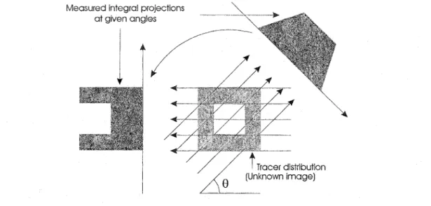
Tomographie data are object "views" or "projections" at different angles. Given PET projection data, one has to obtain the underlying emission density that could have been the source of acquired projections (see figure 1). This would be an approximation to the actual tracer distribution in the subject. The emission density map is also called an

image since it is common to have it visualized after reconstruction.

Measured integral projections at given angles

8

t

Tracer distribution (Unknown image)

Figure 1. Simple case of radiotracer distribution and two idealized continuous projections at selected angles. Projections are shown as if they were not corrupted by the factors inherent to PET data acquisition. Note that projections at angles

e

and

e

±

180° are identical.

(24)

In a broad sense, an inverse problem arises when making inference about a quantity that cannot be observed directly. In tomography, acquired data are used to determine characteristics of a physical phenomenon that cannot be followed otherwise. PET scanners provide projections of the tracer distribution given sufficient time to collect enough coincidence events, which are also referred to as counts. The most likely tracer distribution within the subject being imaged must be derived with dedicated mathematical methods using acquired projection data.

Solution of a tomographie inverse problem is the subject of image reconstruction and provides an image estimate. There are a number of different image reconstruction approaches that have been developed to date including many minor variations. This will be clarified further in Chapter 2, but first let us briefly outline the apparatus of image reconstruction, starting with the PET inverse problem, i.e. the mathematical problem that has to be solved.

1.2.1. Radon transform model

The first published work elaborating on the inverse problem similar to that of CT was by Radon in 1917 (Radon, 1986). He found a solution to the problem of determining a function of two variables from a set of its straight-line integral values.

Let x

=

(xl' xz) E R 2 be a point, line Lp,e be g1ven by equation X1 cos

e

+

X2 sine

=

p ' and the line integral of a real fonction

f (

X1 'X2) along Lp,8 be given by

=

(25)

With some assumptions Radon proved that the fonction

f

could be uniquely determined from the complete set of integral projections, i.e. when R8

(p)

is known for all possible

lines L p, _{8 ,}i.e. with infinitely fine sampling at all possible angles. The problem posed in the Radon's paper is not applicable to PET directly, since a complete (infinite) set of projections is not available in practice and infinitely thin LORs are not best suited for robust modeling of system response, but his approach became the basis for a number of practical image reconstruction techniques. Integral fonctional (1.2.1) is known as the

Radon transfonn of the fonction f . When XE Rn and L is any line in Rn ' the integral

RL

=

J

J(x)dx, (1.2.2)

L

of which (1.2.1) is a special case, is known as the X-ray transform (Louis and Natterer, 1983).

1.2.2. Functional semidiscrete model

Though an idealized problem formulation based on the Radon (and the X-ray) transform was adopted in PET first, better modeling of underlying physical processes requires replacing it with a more sophisticated photon detection model. The following continuous-to-discrete mapping involving a set of simultaneous integral equations can be appropriate (e.g. Baker et al., 1992):

n(d)

=

J

r(d,x)J(x)dx, d

=

1,N. (1.2.3)

Q

where x E .Q

c

Rn is a point of an Euclidean n-dimensional space ( n

=

2 or n

=

3 ), the

(26)

compact, J(x) is the unlmown emission density, r(d,x) is the kemel specified by a model of PET detection process - a spatially varying system response to a source located at point x for the detector pair having index d, n(d) is the number of counts acquired with the detector pair having index d, and N is the total number of active detector pairs. We assume that all N detector pairs are ordered so that a unique pair is referred to by specifying a unique index d. This is in contrast to a more conventional way of having projection angle e and bin position p in a projection n(p,e) as two separate parameters. Single equations in (1.2.3) are varieties of the first-kind Fredholm integral

equation, if strict equalities are assumed (Hansen, 1992).

Qui te generally an image may be viewed as a vector in the Hilbert space" L2

(Q),

where L₂

(Q)

denotes the space of square-integrable functions ** defined over

Q

(Louis and Natterer, 1983). L2

(Q)

would be the image space in this case.

The dynamic aspect of PET sometimes reqmres time as the fourth image dimension, i.e. J(x,t), where tE [a,b] and 0 ~a< b < 00 •

1.2.3. Stochastic extension ofthefunctional model

It is intuitively clear that the true continuous emission map is impossible to recover using the finite number of projections, and one faces a problem that is characterized as ill posed. "An ill-posed experimental problem is one for which there is not as much information in your experimental data as you really need to find out what you want to

Hilbert space is a complete vector space in which a norm and a scalar product are defined.

** Function

J(x)

issquare-integrableover .Q if

flf(x)l2tb:<

00

(27)

know" (Wahba, 1987). By a more rigorous definition of Hadamard, a problem is well

posed if the solution exists, is unique, and depends continuously on the data, otherwise, a problem is ill posed (Franklin, 1970).

True projections are not available due to the physical nature of emission scanning. Many factors contribute to the corruption of projections as mentioned in section l.l. Thus, having equality in (l.2.3) would be next to impossible. An additional zero-mean error vector

e(d),

d

=

l,N is introduced into the deterministic model (l.2.3) to bring it

to equality:

n(d)=

J

r(d,x)J(x)dx+e(d), d =l,N. (l.2.4)

Q

It is also commonly assu111ed that the noise e(d), d

=

l,N can be represented with uncorrelated stochastic variables having some (probably unknown) probability distribution.

1.2.4. Stochastic model

The process of measuring tomographie "projections" in ECT is stochastic in nature.

It is widely accepted that the Poisson distribution* describes the counting statistics for large quantities of radioactive nuclei. The importance of taking into account the stochastic data errors during image reconstruction was pointed out as early as in mid-1970s (Rockmore and Macovski, 1976). Thus, a statistical model of the PET inverse problem has been proposed (Shepp and Vardi, 1982; Vardi et al., 1985):

* Poisson distribution gives the probability of observing x events given the average number of events µ per

time interval according to P(x;µ)

=Le-µ.

(28)

E[77(d)] =

J

p(djx)l(x)dx, d

= 1,N,

(1.2.5)

Q

where

l(x)

is the unknown emission density at point

x

and is assumed to be the mean of an independent random variable (r.v.) having the Poisson distribution,

p(djx)

is the probability of an emission at point x being registered by the detector pair d,

E[77(d)]

is the expected value of r.v.

77(d).

The number of counts acquired with the detector pair d

gives one sample

n(d)

of

77(d),

and

l(x)

has to be estimated.

77(d),d=l,N

are independent Poisson r.v. as well.

1.2.5. Poisson vs. Gaussian data

In practice one records data that are limited by the properties of detection system as well as contaminated by the non-negligible effects of the associated physical phenomena mentioned in section

1.1. A

practical conclusion is that PET data are not expected to be purely Poisson. Indeed, it was shown that data precorrected for random coïncidences may be approximated by the Gaussian distribution* (Fessler, 1994). Moreover, it is known that the Poisson distribution could be hard to tell from the Gaussian distribution for large values of the mean. This "large" mean is not that large in practice, e.g. (Bevington and Robinson, 1992) advises that "for values of the mean greater than about 10, the Gaussian distribution closely approximates the shape of the Poisson distribution." This provides an option of assuming the normal data error distribution, at least under the

* Gaussian (or normal) distribution gives the probability of obtaining value x according to the following

(x-µ)'

law: P(x; µ,a)= ~ e - 2 "2 , where µ is the mean and a is the standard deviation.

(29)

mentioned conditions. Therefore, the left-hand side of (1.2.5) could be changed to accommodate these two cases:

w(d)=

J

p(dlx)/l,(x)dx, d = l,N. (l.2.6)

.Q

The expectation m(d) could correspond to either Poisson or Gaussian distribution and this choice may be made based on the analysis of the data sample at hand. The applicability range could be derived and the validity of the resulting solution would depend on the fulfilment of the underlying assumption on the data nature. It should be noted that a Poisson distribution is easier to describe as it is fully defined by its mean, which is equal to its variance. However, the Gaussian distribution is somewhat more convenient and a considerable number of mathematical methods developed for other applications have been (or could be) transferred to tomography. See Appendix A for an additional explanation.

1.2.6. Deterministic vs. stochastic modeling

Equations (1.2.3) and (l.2.6) have seemingly similar appearance, but they are distinct conceptually and the major difference is in the assumptions on the measured data vector. The former is considered deterministic, whereas the latter represents the

stochastic model of PET. Equation (1.2.4) is the bridge connecting the two. Note also that

/l,(x)E

L2

(.Q)

since the support is bounded and the r.v. mean is finite in any practical

situation. The system response r(d,x) may be easily translated to probabilities p(dlx) with an appropriate normalization.

(30)

A model of PET data acquisition must be set forth as it entails the logic of getting a reasonable solution to the inverse problem. Based on the adopted formulation of the PET inverse problem, (approximate) solution of the set of simultaneous equations (1.2.3) or (1.2.4) or (1.2.6) is the subject of PET image reconstruction. The symbols A and

f

will be used hereafter to denote an image to emphasise its statistical or functional properties, respecti vel y.

Image reconstruction is just an intermediate step in deriving definitive knowledge from PET data. Therefore, it is pointless to argue which model is the best one when detached from the context. The assessment could be performed by comparing reconstruction results on the basis of objective (quantitative) image estimation parameters as well as based on the subjective suitability for providing reliable and conclusive results. Minor objective improvements in image quality do not always lead to improved subjective interpretation of reconstructed images. It is known that the change of inverse problem formulation accompanied by the appropriate change of the image reconstruction method does not necessarily yield clinically important changes in the image estimate. Therefore, either model may be justified if respective assumptions on the data nature are closely satisfied.

1.3. Discrete image and quadrature options

The space L2

(Q)

is separable, i.e. any object

g(x)E

L2

(Q)

can be represented as

an infinite series (Barrett, 1999):

=

g(x)= Lg

1

ljf;(x),

(1.3.1)

(31)

where { l/f; (x )} is the orthonormal basis for L₂

(.Q),

i.e.

(1.3.2)

where

snm

is the Kronecker delta function:

Ônm = ' _{1 _0,n =m

n :f. m (1.3.3)

The coefficients in the series are given by the scalar product

(1.3.4)

A number of image reconstruction techniques use discrete image representation right from the start, i.e. with the inverse problem formulation. Remembering that an image can be represented as an infinite series (1.3.1), one may choose to approximate it with a finite number of basis vectors for simplicity. lt is possible to use a non-orthogonal basis as well, e.g. functions ~;

(x ),

i

=

1, M spanning some space

(Q).

It is preferable to have

(Q)c

L2

(Q),

which is automatic if ~;(x)E L2

(Q)

for all i.

(Q)

is the image representation space. The linear approximation to the image in this case would be

M

J(x)=

L/;~;(x), (1.3.5) i=l

where ~;

(x)

are not necessarily normalized and orthogonal, M is the total number of

these functions. The functions ~; (x) are called expansion functions to distinguish them

(32)

A common practical method of obtaining a set of expansion functions involves representing the support Q with a set of smaller compact regions Q_{1 ,}called pixels in

2-D and voxels in 3-2-D case. The unity

U

of ail pixels• must con tain Q :

(1.3.6)

A pixel Q; may serve as the support for an expansion fonction f/J;

(x)

in the simplest case, and the value of f/J;

(x)

is assumed constant over Q;. This simplistic approach Jacks theoretic justification and poses the problem of pixel grid optimization, however, the set of expansion functions would be automatically orthogonal if defined on non-overlapping pixels. These can be conventional square pixels of the same size, or a more complicated set of polar pixels may be used (Kearfott, 1985; Kaufman, 1987), see figure 2 below for an illustration. fl 1 fl, ··"'·· ··· '• "

n

.·

Figure 2. From left to right: a) an example of the support region Q, which is the ellipse interior; b) a set of conventional square pixels; c) a set of polar pixels.

A grid of square pixels is very suitable for subsequent image visualisation with digital displays, therefore it is most widely utilised in practice. Another attractive alternative is

• The description given hereafter will be limited to the 2-D case to simplify examples but without loosing generality.

(33)

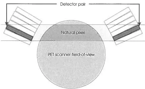
the grid of natural pixels (Buonocore et al., 1981) that is easy to appreciate from the following explanation. Any two opposite detectors in the ring can register annihilation photons originating only from a compact region which is usually significantly smaller than the support Q but large enough to be poorly represented by a single infinitely thin

line connecting two detectors as the Radon transform model implies. A compact region that actually represents the FOV of two given detectors is called a tube-of-response

(TOR). An example of a strip TOR model is shown in figure 3.

Detector pair

Figure 3. Tube-of-response for a given detector pair. It is assumed that the two detectors in the ring are able to register coïncident annihilation photons originating from any point of the tube-of-response. The model may be applied in 2-D image reconstruction.

TOR is a more realistic detection model for PET as compared to LOR. The inverse problem can be written using the TORs. The model (1.2.6) becomes, for instance:

m(d)=

J

p(dlx)A(x)dx, d =l, ... ,N, (1.3.7)

sd

where S d is the TOR corresponding to the detector pair d. The intersection of a TOR

with the PET scanner FOV yields a natural pixel and is shown in figure 4. An orthonormal pixel basis based on natural pixels has been proposed in (Baker et al., 1992).

(34)

Detector pair

t\Jatural pixel

PET scanner field-of-vlew

Figure 4. Natural pixel defined as an intersection of the tube-of-response shown in the previous figure and the PET scanner field-of-view.

It is possible, however, to define a convenient set of expansion functions to facilitate the problem solution and expand the solution in another set afterwards if need arises. A multitude of candidates for expansion functions are feasible, e.g. a set of spherically symmetric volume elements (blobs) was proposed (Lewitt, 1992; Matej and Lewitt, 1996) to simplify calculation of image projections and to have contrai over image smoothness properties.

The choice of a pixel grid is an important one, especially when a system with unconventional geometry is used for data acquisition. An improper choice would result in unnecessary complications aggravating the issues of solution stability and uniqueness. Irrespective of the choice of expansion fonctions, however, the final image is remapped to conventional square pixels to facilitate image display and sharing in digital form.

(35)

1.4. Image projection

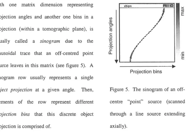
An idealized illustration of continuous object projections in 2-D was given already in figure 1. Actual raw PET data are a finite set of numbers representing the number of counts acquired in a given TOR over time. This set of values, arranged in a 2-D matrix with one matrix dimension representing

projection angles and another one bins in a projection (within a tomographie plane), is usually called a sinogram due to the

sinusoïdal trace that an off-centred point source leaves in this matrix (see figure 5). A sinogram row usually represents a single

object projection at a given angle. Then,

elements of the row represent different

projection bins that this discrete object

projection is comprised of.

(/) Q) O> c:: CU c:: 0

·g

Q>

·e-a.. xhips l!ll!IEI

J

/,/'

.:·

,

..

/

•

Projection bins >< CU E

Figure 5. The sinogram of an off-centre "point" source (scanned through a line source extending axially).

PET imaging may be quite generally modelled with the continuous-to-discrete mapping P : L₂

(Q )---7

RN as discussed in section 1.2. The linear operator P is bounded, i.e. there exists a positive number c such that

llPJll

<

cilJll

for ail

f.

However, its inverse is unbounded and P is often substituted with its discrete counterpart P0 :

(Q)---7

RN for practical purposes. When computed for a given PET system, P0 is

(36)

integral equations (1.2.3) and (1.2.4) can be reduced to the following matrix forms, respectively:

n=.Pf. (1.4.1)

and

n =Pf +E. (1.4.2)

where n is an N-dimensional vector of projection data; the matrix P is comprised of

probabilities, i.e.

N

LPu

=l, j=l,M, (1.4.3)

i=l

which are obtained by the normalization of the system response model, and

f

=

{f; : i

=

1, M} is the set of expansion coefficients characteristic for the image approximation expressed as the finite series (1.3.5).

The statistical model (1.2.6) can be represented as the system of linear equations just the same way:

(J)=PA, (1.4.4)

where

m

is an N-dimensional vector of expectation of a Poisson or Gaussian r.v. as discussed in section 1.2.5, and A= {;t;: i

=

l,M} is the set of expansion coefficients representing the image.

One should keep in mind that the actual incarnation of operator P is determined by the physical modeling for a particular scanner and the chosen image representation. Different photon detection models as well as other relevant physical phenomena

(37)

associated with the system response model will, generally, yield distinct matrices P. The modeling of the system response is called the direct problem, and is an essential part

of solving the inverse problem. The matrix P, approximating operator P, is called

either the system matrix or the transition matrix*. The system matrix is usually very

sparse, i.e. has many zero entries. This is mainly due to the modeling that assumes that TOR covers a finite space region, which is much smaller than the FOV (see figure 4); hence, a given TOR might see only a fraction of the set of local expansion functions. That happens if expansion functions are localized. Image projection becomes as simple as mapping R M into RN with the help of the system matrix if P <1> is set.

1.5. Backprojection

Another essential operation has yet to be introduced, which is refeITed to as the

backprojection. It is the adjoint of image projection described in the previous section and

maps from the finite dimensional projection space to the infinite dimensional image space, i.e.

pt:

RN -7 L₂

(.Q)

(Natterer, 1980):

N

(ptg)(x)=

Lg;X;' (1.5.1)

i~l

where g; are the weights and

( ) {1, XE Sd X X=

' 0, otherwise (1.5.2)

* The term "projection matrix" can be met as well. However, one should not think of the system matrix as a projector, in terms of the theory of matrix operators. A real valued projector must be symmetric and idempotent, i.e. P =PT and P2 ₌_{P, respectively, and the system matrix generally does not qualify.}

(38)

The discrete counterpart of the backprojection operator P~ : RN --7

(Q)

is

employed if one has chosen to use practical image approximations. Therefore, assuming that the same image representation is used for backprojection as for projection, the backprojection operator will be approximated by the transpose of the system matrix pT, since for a real matrix the adjoint and transpose are synonymous. Thus, with the image approximation given in

(Q),

image backprojection is as simple as mapping RN back into RM.

1.6. System matrix properties and inverse problem analysis

The challenges of the inverse problem solution can be directly associated with the properties of the respective projection operator P. Getting rid of the problem ill-posedness could be a sufficient reason for representing a continuous image as a finite series, however this approximation does not necessarily convert the inverse problem into a well posed one in the sense of Hadamard. Sorne insight can be gained by examining the projection operator or its discrete approximation - matrix P.

Several important definitions have to be recalled first. The set of all vectors that the operator P act upon is called the domain of P . The range of operator P is defined as the set of all vectors g that can be reached by applying P to the members of a given

functional space, i.e. :o/i(P) = { g : g = Pf, for some f from the domain of P }. The

nullspace of operator P is defined as the set of all fonctions that are mapped to zero, i.e.

cJf/(P)

=

{f : Pf

=

0}. The same definitions are applied to matrices that are considered in the case of discrete-to-discrete mapping. The operator P is injective, or one-to-one, if each vector of the original functional space is mapped to a single vector in :o/i(P) . The

(39)

operator P would be surjective, or onto, if all vectors of the target space would be in the range

9't(P).

The operator

P

is invertible if it is injective and surjective. The nullspace of an invertible operator is trivial, i.e.

G/V(P) = {

0}. The operator that is not invertible is said to be singular. The real-world imaging operators are always singular (Barrett, 1999).

A powerful approach to inverse problem analysis involves the singular value

decomposition (SVD) of the projection operator. Here we will describe the discrete case only since it is directly relevant for the following presentation. The application of SVD to the analysis of continuous-to-continuous mapping may be found in (Davison, 1983; Louis, 1986; Caponnetto and Bertero, 1997).

It is well known that any NxM matrix P can be decomposed into a product of three

special matrices (Strang, 1980):

P=UDVT, (1.6.1)

w here D

=

diag

(µ

1 , µ2 , ••• , µ M ) is a diagonal matrix of singular values,

U

=

(uij

ti.N;

j=l,M is an NxM matrix with orthonormal columns, that are referred to as the

left singular vectors u_1.

=

u.₁

=

(u;;} - ,

_{, r=l,N} V

=

(v;;) - . -

_{, r=l,M; J=l,M} is an MxM matrix with orthonormal columns, that are referred to as the right singular vectors v j

=

v.j

=(vu

)i=l,M.

The factored representation (1.6.1) is known as the matrix SVD. The left singular vectors

u j corresponding to the non-zero singular values form an orthonormal basis spanning the

range of P. The right singular vectors v j corresponding to the zero singular values form

(40)

related via

Pv. _J=µ _.!u. _J (1.6.2)

and

(1.6.3)

The set of singular values is called the singular value spectrum. The singular

values are usually ordered so that

(1.6.4)

The decay rate of the singular values is an important indicator of information content for the inverse problem (Gilliam et al., 1990; Wahba, 1980). In case of continuous mapping,

the problem is mildly ill posed if the singular values decay slowly and there is a good

chance of finding a stable (approximate) solution. The problem is severely ill posed and

calls for a dedicated solution technique if the singular value spectrum drops towards zero rapidly. The ratio

(1.6.5)

is referred to as the matrix condition number and is a simple measure of the degree of

inverse problem ill-posedness. A matrix is singular if CP

=

oo. If the matrix is not

singular but the condition number is significantly large, the matrix is said to be ill

conditioned. The inverse matrix p-i would have a very large norm in that case, which

would result in huge amplification of minor perturbations. The singular values are also directly related to the eigenvalues*

ai

of the self-adjoint matrix pT P (hence, ppT as

(41)

well), which appears in the normal equations*, and

(1.6.6)

The problem (1.4.1) could have an exact solution if n E

:c?ll(P).

Unfortunately, that

is usually not the case and one has to settle with an approximate (generalized) solution

f+, which can be chosen according to some optimality criterion.

1.

7. Regularisation

The presence of noise in projection data is not the only challenge inherent to the PET inverse problem as we have seen already. Special methods have to be employed when handling severely ill posed (or ill conditioned) problems that involve replacing the initial problem with another one having more favourable properties. This technique is called regularisation. Following (Bertero et al., 1988), we define a regulariser for our inverse problem.

Let p+ be an operator that gives a generalized solution to (1.2.3) or (1.2.4):

(1.7.1)

A family of linear operators { P;

L>o,

P; : RN -7 L₂

(Q)

constitute a regulariser for an operator p+ if the following conditions are satisfied:

(i) for any w > 0,

:c?ll(P;)

c

<l>(Q);

Normal equations arise with the least-squares approach to approximate solution of an optirnization problem.

(42)

(iii) lim P; =P+.

W->0

Thus P; is a regularised approximation of p+ and the variable w is called the regularisation parameter. Choosing the most appropriate value of w is one of the main problems of regularisation theory. A useful overview of the image reconstruction problem and regularisation can be found in (Demoment, 1989).

(43)

Chapter 2. Image Reconstruction Techniques

Various inverse problem models could describe PET imaging as has been discussed in section 1.2. A variety of established mathematical tools and numerical algorithms can be utilised to derive a reasonable solution - a feasible image approximation, even if the inverse problem formulation stays the sarne. Thus, a great number of image reconstruction algorithms have been conceived. An overview given in the present chapter will clarify current state-of-the-art. The reviews given in (Natterer, 1999) and (Leahy and Qi, 2000) cover somewhat different perspectives and may be a brief introduction to the subject as well.

2.1. General Classification

The primary differences among reconstruction techniques stem from the adopted formulation of the PET inverse problem. This leads to two broad classes of algorithms, namely deterministic and statistical, based on the respective inverse problem models discussed in section 1.2. The choice of discrete or continuous image model differentiates

series-expansion from transform methods, respectively. Yet another fundamental distinction arnong algorithms exists: they may be classified in one-step and iterative groups. One-step reconstruction methods aim at solving the inverse problem at a single (though complex) step, thus providing a "final" image estimate, whereas iterative methods attempt to reach a solution by successive improvement of an image estimate starting with some initial guess.

This classification clarifies underlying concepts, but image reconstruction algorithms might fall into several categories at the same time as the corresponding

(44)

classification reflects different and non-exclusive properties. Moreover, the boundaries between the opposite groups are sometimes vague. A deterministic model having no solution in the sense of Hadamard, for instance, may be solved approximately in the least-squares sense* and may involve statistical interpretation of data errors. A solution expanded into the set of eigenvectors of the system matrix can be related to conventional Fourier techniques (Llacer, 1979). A similar relationship has been studied in (Anastasio

et al., 2001) for the continuous case.

Another perspective onto the image reconstruction problem is presented in figure 6. Two alternative routes that employ regularisation atone stage or another may be taken to derive a "solution". Either the operator P is replaced by its discrete counterpart P which, in turn, is replaced by a regularised version

Pw, or the operator P is idealized (the

Radon's approach 1s an example) and its regularised version Pw is studied completely

m functional spaces and a numerical _{Figure 6. Diagram showing two} approximation is developed that involves _{alternative routes that could be} discretisation Pw of the regularised operator _{taken when solving an inverse}

after that. problem approximately.

Function f is a least-squares solution of Pf = n if inf {jjPu - njj : u E X}=

lift -

njj . The solution

(45)

It should be mentioned that the idealisation of P with the help of the Radon transform was studied first and the most. The powerful set of transform methods is the widely used result of developments with the Radon (or X-ray) transform. However, the series expansion approach employing early image discretisation is used more often in current research.

2.2. Summation Method

The easiest tomographie reconstruction method is the one called summation or back projection, due to the simple superposition of projections by spreading them back across the reconstruction plane. This would involve a single operation of backprojection introduced in section 1.5. The summation method yields image estimates that are blurred and the degree of blurring in the case of an infinite number of angles and the line integral measurement model is proportional to

1/

r, where r is the distance from the point source of radioactivity. For more details see e.g. the review in (Gordon and Herman, 1974).

Though it is hardly used as a standalone reconstruction method in practice, the backprojection operation is an essential part of most practical image reconstruction techniques. Efforts have been made to improve backprojection algorithms (Peters, 1981; Cho et al., 1990; Egger et al., 1998) along with designing special hardware for backprojection (Thompson and Peters, 1981; Hartz et al., 1985; Jones et al., 1990) to accelerate reconstruction.

(46)

2.3. Transfonn Methods

A distinct set of image reconstruction techniques 1s based on the Fourier

transfonn*, which in 2-D is defined as:

1 = = .

oY{f

=

[~J

](u, v) = -

J J

f(x, y )e-i(ux+vy)dxdy,

2n -=-=

(2.3.1)

where

f

(x,

y)

is the image fonction, and i2

=

_-1. _{A single projection at angle}

e,

_when

subject to the one-dimensional (1-D) Fourier transform

(2.3.2)

yields a central section of the 2-D Fourier transformed image at angle

e :

[@

2

f

](wcosB, wsinB) =[~Re ](w ),

(2.3.3)

This relationship is referred to as the projection slice theorem, or the central slice

theorem, or the Fourier slice theorem (Kak and Slaney, 1988).

A number of techniques employing Fourier transforms have been described. Reconstruction may be accomplished by transferring projections into the Fourier space, interpolating in the frequency domain to get the sampling on a square grid, and then transferring the resulting frequency estimate back into the image space with the inverse

Fourier transform, which in 2-D will yield:

* The Fourier transform is defined as ](ç)

=

[~J Kç)

=(2;rtN

12

J

J(x)e-;çdx;

the inverse Fourier

RN

transform is defined as l~-1]

Jx)=(2;rr

12

f

j(Ç)é'dÇ.

(47)

f

(x,

y)=

o~-l

J

@;R₀d(} . (2.3.4)

27t

This approach is referred to as direct Fourier method (DFM). The major problem with

DFM is the robust interpolation in the Fourier space to resample the points from polar to Cartesian grid, which results in image artefacts if a simplistic interpolation strategy is employed. For the latest developments with DFM see (Waldén, 2000; Gottlieb et al.,

2000).

Another approach is termed the convolution method and is based on the fact that the

Fourier transform of the convolution of two functions * equals the product of their indi vidual Fourier transforms

(2.3.5)

This leads to practical reconstruction techniques, since the measured emission data represent "ideal" projections convolved with the system point spread function (PSF)**. One popular algorithm starts with transferring each measured projection into the Fourier space, applying an appropriate filter to de-convolve the effect of image blurring ( observed with the summation method), then transfers the result back into the projection space, and finally, backprojects the filtered projections onto the image grid. This technique is called filtered backprojection (FBP). The following equation can be an

illustration:

jFBP(x,

y)=

L:Backproject{@;-

1 [

c(w)x@;R

_{8; ]}.}

(2.3.6)

B;

* Convolution of 1-D fonctions

çt>(v)

and

ip(v)

is defined as

[çt>

*

q> ](v)

=

f

çt>(u )ip(v - u )du .

(48)

It is customary to put a hat over

f ,

to recognise the fact that this is an approximate solution, i.e. an image estimate. In (2.3.6), R8 1 is the projection at angle B; sampled at a

finite number of points, i.e. R8; is a single row of the sinogram (as discussed in section

1.4), and

c(w)

is a 1-D fonction, a sampled version of a window of the ramp

filter c(w)

which arises as a correction for non-uniform sampling in the Fourier domain and is given by

c(w)

=

{1 wl, lwl::;

Wmax .

0, 1

wl

> Wmax

(2.3.7)

Here wmaxis the eut-off frequency, which is determined from the given sampling with the Radon transform. This relationship stems from a result of the sampling theory that is known as the Nyquist sampling rate, which states that a signal must be sampled at least twice during each cycle of the highest frequency of the signal.

Extensive treatment of FBP theory and implementation is given in (Rowland, 1979; Budinger et al., 1979; Kak and Slaney, 1988). FBP is currently the algorithm of choice in most practical applications due to its overall acceptable performance and relative computational simplicity, due to availability of efficient implementations of the fast Fourier transform and 1-D operations involved. Another ordering of backprojection, filtering and the Fourier transform is possible and would result in a different algorithm:

(2.3.8)

Topics in image reconstruction for high resolution positron emission tomography

UNIVERSITÉ DE SHERBROOKE

TOPICS

IN

IMAGE RECONSTRUCTION FOR

HIGH RESOLUTION POSITRON

EMISSION

TOMOGRAPHY

par

Vitali Selivanov

Département de Médecine nucléaire et de radiobiologie

Thèse présentée à la Faculté de médecine

en vue de l'obtention du grade de

philosophiae doctor (Ph.D.) en radiobiologie

Sherbrooke (Québec) Canada

2002

l+I

The author has granted a

non-exclusive licence allowing the

National Library of Canada to

reproduce, loan, distnbute or sell

copies of this thesis in microfonn,

paper or electronic formats.

The author retains ownership of the

copyright

in

this thesis. Neither the

thesis nor substantial extracts :from it

may be printed or otherwise

reproduced without the author' s

penmss10n.

L'auteur a accordé une licence non

exclusive permettant

la

Bibliothèque nationale du Canada de

reproduire, prêter, distribuer ou

vendre des copies de cette thèse sous

la

forme de microfiche/film, de

reproduction sur papier ou sur format

électronique.

L'auteur conserve

la

propriété du

droit d'auteur qui protège cette thèse.

Ni

la

thèse

ni

des extraits substantiels

de celle-ci ne doivent être imprimés

ou autrement reproduits sans son

autorisation.

Contents

Abbreviations

List of Figures

List of Tables

Abstract

>-

>-

Résumé

Introduction

Chapterl. Background

1.1. Principles of PET

v -

1.2. PET inverse problem

t

e

e

±

=

e

+

=

f (

f

(p)

=

J

=