Analyse fréquentielle régionale mutivariée basée sur le modèle de l'indice de crue.

ANALYSE FRÉQUENTIELLE

RÉGIONALE MULTIVARIÉE

BASÉE SUR LE MODÈLE

DE L'INDICE DE CRUE

ANALYSE FRÉQUENTIELLE RÉGIONALE MULTIVARIÉE

BASÉE SUR LE MODÈLE DE L'INDICE DE CRUE

F. Chebana* and T.B.M.J. Ouarda

Industrial Chair in Statistical Hydrology/Canada Research Chair on the Estimation of Hydrometeorological Variables,

INRS-ETE, 490 rue de la Couronne, Quebec (QC) Canada G1K 9A9

Rapport de recherche R-1076

TABLE OF CONTENT

TABLE OF CONTENT ... III  ABSTRACT ... V 

1  INTRODUCTION AND LITERATURE REVIEW ... 1 

2  BACKGROUND ... 5 

2.1  Univariate index-flood model ... 5 

2.2  Multivariate quantiles ... 6 

3  MULTIVARIATE INDEX-FLOOD MODEL ... 11 

4  PERFORMANCE EVALUATION USING SIMULATION ... 15 

4.1  Simulated regions ... 15 

4.2  Performance evaluation criteria ... 19 

4.3  Simulation procedure ... 22 

5  RESULTS ... 25 

5.1  Preliminary simulations ... 25 

5.2  Main results ... 27 

5.3  Effect of various factors on the estimation results ... 30 

6  CONCLUSIONS AND FUTURE WORK ... 33 

ACKNOWLEDGMENTS ... 35 

NOTATION LIST ... 37 

BIBLIOGRAPHY ... 39 

ABSTRACT

Because of their multivariate nature, several hydrological phenomena can be described by more than one correlated characteristics. These characteristics are generally not independent and should be jointly considered. Consequently, univariate regional frequency analysis (FA) cannot provide complete assessment of true probabilities of occurrence. The objective of the present paper is to propose a procedure for regional flood FA in a multivariate framework. In the present paper, the focus is on the estimation step of regional FA. The proposed procedure represents a multivariate version of the index-flood model and is based on copulas and a multivariate quantile version with a focus on the bivariate case. The model offers increased flexibility to designers by leading to several scenarios associated to the same risk. The univariate quantiles represent special cases corresponding to the extreme scenarios. A simulation study is carried out to evaluate the performance of the model in a bivariate framework. Simulation results show that bivariate FA provides the univariate quantiles with equivalent accuracy. Similarity is observed between results of the bivariate model and those of the univariate one in terms of the behaviour of the corresponding performance criteria. The procedure performs better when the regional homogeneity is high. Furthermore, the impacts of small variations in the record length at gauged sites and the region size on the performance of the proposed procedure are not significant.

1 INTRODUCTION AND LITERATURE REVIEW

Extreme events, such as floods, storms and droughts have serious economic, environmental and social consequences. It is hence of high importance to develop the appropriate models for the prediction of such events both at gauged and ungauged sites. Local and regional frequency analysis (FA) procedures are commonly used tools for the analysis of extreme hydrological events. The objective of regional frequency analysis (RFA) is to transfer information from gauged sites to an ungauged target site within a homogeneous region.

Generally, hydrological events are characterized by several correlated variables. For instance, floods are described through their volume, peak and duration (Ashkar, 1980; Yue et al., 1999; Ouarda et al., 2000; Yue, 2001; Shiau, 2003; De Michele et al., 2005; Zhang and Singh, 2006; Chebana and Ouarda, 2008b). These studies have pointed out the importance of jointly considering all these variables. Depending on data sources and the number of variables that characterize the event, frequency analysis can be divided into four classes: univariate-local, univariate-regional, multivariate-local and multivariate-regional. The first two classes have been extensively studied, see e.g. Stedinger and Tasker (1986), Burn (1990), Hosking and Wallis (1993), Durrans and Tomic (1996), Nguyen and Pandey (1996), Alila (1999, 2000), Ouarda et al. (2001, 2006) and Chebana and Ouarda (2008a). Recently, increasing attention has been given to multivariate-local FA e.g., by Yue et al. (1999), Yue (2001), Shiau (2003), De Michele et al. (2005), Zhang and Singh (2006) and Chebana and Ouarda (2008b). However, much less attention is given to multivariate-regional FA. In this category, we find few references such as Ouarda et al. (2000) and Chebana and Ouarda (2007).

Justifications for adopting the multivariate framework to treat extreme events were discussed in several references. In bivariate FA, Yue et al. (1999) concluded that single-variable hydrological FA can only provide limited assessment of extreme events. A better understanding of the probabilistic characteristics of such events requires the study of their joint distribution. It was also outlined in Shiau (2003) that multivariate FA requires considerably more data and more sophisticated mathematical analysis. Univariate FA can be useful when only one random variable is significant for design purposes or when the two random variables are less dependent. However, a separate analysis of random variables cannot reveal the significant relationship between them if the correlation is an important information in the design criteria. Therefore, it is of importance to jointly consider all the random variables that characterize the hydrological event.

Three main elements are treated in multivariate-local FA literature: (1) explaining the usefulness and importance of considering the multivariate framework, (2) modeling extreme events by fitting the appropriate copula and marginal distributions, and estimating the corresponding parameters, and (3) defining bivariate return periods. However, despite the importance of quantiles in FA, the literature on multivariate-local FA did not specifically address the estimation of multivariate quantiles. Recently Chebana and Ouarda (2008b) introduced the notion of multivariate quantile in hydrological FA.

Regional FA is generally composed by two main steps: regional delineation and extreme quantile estimation (see e.g., GREHYS, 1996a). In the multivariate context, the delineation step was treated in Chebana and Ouarda (2007) where multivariate discordancy and homogeneity statistical tests were proposed. In univariate-regional FA different quantile estimation methods were proposed in the literature, such as the index-flood method and regressive models (see GREHYS, 1996a,b). As a natural continuation of the study by Chebana and Ouarda (2007) and in

order to present a complete multivariate-regional FA framework, an estimation procedure in the multivariate context is presented in this paper. The present procedure is an extension of the index-flood model to the multivariate context.

The multivariate index-flood model is based on two main concepts: multivariate quantile curves and the notion of copulas. The univariate index-flood model aims to obtain an estimation of quantiles at ungauged sites using data (and hence quantiles) from sites within a specified region. The objective of FA is the quantile estimation which can be obtained through the cumulative distribution function or the density function. The multivariate quantile version adopted in this paper is a curve composed of combinations of the variables corresponding to the same risk. Copulas are employed in order to model the dependence between the variables describing the event.

The paper is organized as follows. In Section 2, we present some background elements required for the development of the methodology: the index-flood model and multivariate quantile curves. In Section 3, we present the multivariate-index flood model. In Section 4 a simulation study is carried out to evaluate the performance of the proposed model with an adaptation of the procedure to flood events. Results and discussions are reported in Sections 5 and 6 respectively, whereas the conclusions are presented in the last section.

2 BACKGROUND

The principal elements required for the development of the proposed estimation procedure are presented in this section; namely, the univariate index-flood model and bivariate quantile curves.

2.1 Univariate index-flood model

The index-flood model was first introduced by Dalrymple (1960). Similar models can also be used for other hydrological variables including droughts and storms (Pilon, 1990, Hosking and Wallis, 1997 and Hamza et al., 2001). In this model the region is assumed to be homogeneous. That is, all sites in the region have the same frequency distribution apart from a scale parameter that characterizes each site. Explicitly, for a region where data are available for N sites, the model gives the quantile Q p corresponding to the non-exceedence probability p at site i as: _i( )

( ) ( ), 1,...,

i i

Q p =μ q p i= N and 0< <p 1 (1)

whereμ_i represents the index-flood and q(.) is the regional growth curve.

The index-flood parameter μ_i may be estimated, for instance, as the sample mean at site i. The growth curve q(.) may be estimated using the standardized data of the whole region. Usually, we assume known the form of q(.) through a regional distribution K(.; )θ except for some parameters θ =

(

θ₁,...,θs

)

. More details about the index-flood model can be found in Hosking and Wallis (1993), and for a more recent review the reader is referred to Bocchiola et al. (2003).

2.2 Multivariate quantiles

In the literature, several studies proposed to extend the well-known univariate quantile to higher dimensions. Serfling (2002) presented a review and a classification of some of these multivariate quantile versions. According to this classification, there are two major categories of multivariate quantiles: vector- and real-valued quantiles. In the vector-valued class, we find multivariate quantiles based on depth functions (Serfling, 2002); multivariate quantiles based on norm minimization defined by Abdous and Theodorecu (1992) and Chaudhuri (1996); multivariate quantiles as inversions of mappings studied by Koltchinskii and Dudley (1996); and data-based multivariate quantiles based on gradients developed by Hettmansperger et al. (1992).

The real-valued quantile class contains the generalized quantile processes introduced by Einmahl and Mason (1992).

More recently, Belzunce et al. (2007) defined another bivariate vector-valued quantile version. This version is not included in the review by Serfling (2002) and is focused on the bivariate context. Let ( , )X Y be an absolutely continuous random vector andp∈]0,1[. The pth bivariate quantile set or bivariate quantile curve for the direction ε is defined as:

{

2

}

, ( , ) ( , ) : ( , )

X Y

Q p ε = x y ∈R F x yε = p (2)

where ( , )F x y_ε is one of the four following probabilities:

{

}

{

}

{

}

{

}

( , ) Pr , , ( , ) Pr , ( , ) Pr , , ( , ) Pr , F x y X x Y y F x y X x Y y F x y X x Y y F x y X x Y y ε ε ε ε ++ +− −− −+ = ≥ ≥ = ≥ ≤ = ≤ ≤ = ≤ ≥

In other words, the bivariate quantile (2) is a curve corresponding to any combination (x,y) that satisfies ( , )F x y_ε = (an infinity of combinations). This definition of the bivariate quantile is p simple, intuitive and does not require any symmetry assumption. Furthermore, the bivariate distribution (copula and margins) appears in its evaluation. A multivariate quantile curve can be obtained for the uniform margins and then transformed using the univariate quantile function of each component. To this end, we introduce copulas as follows. A copula is a description of the dependence structure between two or more random variables. For more details on copula functions, the reader is referred for instance to Nelsen (2006) or to Chebana and Ouarda (2007). Sklar’s (1959) theorem is an important result which provides, for two random variables X and Y, the relationship between their bivariate joint distribution F , the corresponding copula C and marginal distributions F_X and F . Sklar’s result states that there exists a copula C such that: _Y

(

)

( , ) _X( ), _Y( ) for all real and y

F x y =C F x F y x (3)

In addition, if F_X and F are continuous, the copula C is unique. Hence, for the _Y event

{

X ≤x Y, ≤ y

}

, using (2) and (3), the quantile curve can be expressed as follows:

{

2 1 1

}

, ( ) ( , ) such that ( ), ( ); , [0,1] : ( , )

X Y X Y

Q p = x y ∈R x =F − u y =F − v u v ∈ C u v = p (4) Consequently, in the present paper the proposed bivariate index-flood model is based on (4). The resolution of equation (4), using copula and margin expressions, leads to several solutions called combinations. These combinations constitute the corresponding quantile curve.

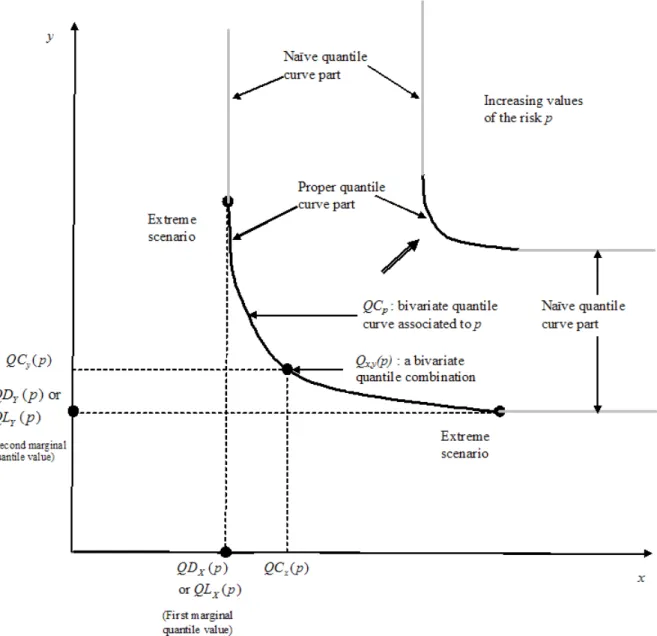
The usual univariate quantiles are special cases of the bivariate quantile curve given in (2) or (4). Indeed, Figure 1 illustrates that the univariate quantiles represent the extreme points of the proper part of the bivariate quantile curve.

The following notations are employed throughout the paper and are illustrated in Figure 1:

p

QC is the bivariate quantile curve associated to a risk p of the non-exceeding event on variables

X and Y which corresponds to QC_{X Y,} ( ,p ε − − of equation (2) (we may denote it by )

, ( )

X Y

QC p if it is necessary to make the emphasis on the variables);

, ( )

x y

Q p represents a point (a combination) of the curve QC ; _p

( ) x

QC p and QCy( )p are the coordinates of the point Qx y, ( )p , that is

(

)

, ( ) ( ), ( )

x y x y

Q p = QC p QC p .

The univariate quantiles are denoted as QD_X( )p and QD_Y( )p when directly evaluated and ( )

X

QL p and QL_Y( )p when deduced as extreme values from the bivariate quantile curve. A complete list of the notations used in the paper is presented at the end of the document.

We close this section by summarizing some key facts that are related to the notion of bivariate quantile in local FA (for more details see Chebana and Ouarda, 2008b):

1. The quantile curves, for practical reasons, are composed of two parts: naïve part and proper part (central part). The naïve part is composed of two segments starting at the end of each extremity of the proper part. These segments are parallel to the axis. The points that define the extremities correspond to the maximum value for each of the variables x and y in the empirical version of the quantile curve or in the case where the marginal distributions are bounded (right or left according to the considered event). In the case of quantiles corresponding to the parent distribution when the margins are not bounded, there are two options to identify the extremities of the proper part. It is possible to take the extremities to

be related to those of the empirical version. It is also possible to select the extremities to be as close as needed to the asymptotes. The first option is useful for the comparison of the empirical and true quantiles. For simplicity, Figure 1 presents the case where the margins are right-bounded.

2. The marginal quantiles correspond to the extreme scenarios of the proper part related to the event.

3. For a given sample, univariate estimation results should be used cautiously since the combination of the univariate quantile values of each variable does not correspond to the desired risk and hence may lead to wrong conclusions.

4. Some events, relating both variables, cannot be expressed in the univariate context.

5. The number of bivariate quantile scenarios in the proper part decreases, when the risk p increases, and hence the proper part of the quantile curve becomes shorter.

These key statements are illustrated in Figure 1. In the remainder of the paper, if it is not specified, the quantile curve refers to the proper part of the full curve.

Generally, explicit or analytical expressions of bivariate quantiles are not available. Hence, bivariate quantiles are obtained numerically by resolving equations (2) or (4). Some difficulties may arise when solving these equations, especially for values of p that are very close to 1 and/or for complex distributions (margins and copula). The procedure employed to obtain multivariate quantile curves is parametric. That is the joint distribution F is shown to belong to a class of parametric distributions with unknown parameters to be estimated. The class of parametric distributions is identified using goodness-of-fit tests. The parametric estimation approach is commonly used in hydrologic FA. In the univariate context some nonparametric approaches have been employed in hydrologic FA (see e.g., Adamowski and Feluch, 1990; Ouarda et al., 2001)

but these methods are of limited use for hydraulic design of major structures as indicated by Singh and Strupczewski (2002).

3 MULTIVARIATE INDEX-FLOOD MODEL

The following procedure represents a complete multivariate version of regional FA. It includes the two main steps: delineation of a homogeneous region and estimation of the extreme event. The step dealing with the delineation of a region is treated in Chebana and Ouarda (2007) who proposed multivariate discordancy D and homogeneity H statistical tests based on multivariate L-moments. The statistic H is also employed as a heterogeneity measure for a given region. The development of the estimation step is the object of the present paper. It consists in extending the index-flood model to the multivariate framework. For notation clarity and computation simplicity, the procedure is presented for the bivariate setting. Nevertheless, the procedure can be conceptually extended to higher dimensions. However, some theoretical and practical elements need to be developed such as copula modeling, parameter estimation and computational aspects. These elements are discussed at the end of the present section.

Given a set of N sites with record length n at site i, i =1,…, N, the problem is to estimate, at the _i target-site

l

, the quantile of interest corresponding to a given risk p, 0< < (or equivalently a p 1 return period T). The data are of the form (x y_ij, _ij) for j = 1,…,n and i = 1,…, N where x and y _i represent realisations of the considered variables. Let qC be the regional growth curve which _p represents a quantile curve common to every site in the region. It can be seen as a “regional quantile curve” and can be obtained on the basis of the standardized data of the whole region. The procedure is described as follows:

1. Identify the set of sites (region) to be used in the estimation as follows (Chebana and Ouarda, 2007):

1.1. Apply the multivariate discordancy test D to identify discordant sites to be removed from the region,

1.2. Check the homogeneity of the remaining sites by applying the multivariate homogeneity test H. Assume these sites are indexed from 1 to N ′(with N′ ≤N).

2. For each site i, i = 1,…, N ′:

2.1. Assess the location parameters μˆ_{i X,} and μˆ_{i Y,} ,

2.2. Standardize the sample (x y_ij, _ij) to be

(

x'_ij =x_ij μˆ_{i X,} , y'_ij = y_ij μˆ_{i Y,}

)

,

3. Select a family of regional multivariate distributions to fit the standardized data of the whole region (x y_ij′ ′ for j = 1,…,, _ij) n and i = 1,…, _i N ′: this includes the marginal distributions as well as a copula. In the present context, assume that the regional distribution depends upon s parameters denoted θ₁,...,θ_s.

4. Estimate the parameters of the distribution obtained in step 3:

4.1. Obtain an estimator θ of the kˆ_k( )i th parameter from the standardized data of the ith site, k = 1,…, s and i = 1,…, N ′. The maximum likelihood method or the L-moments-based method can be used for the estimation.

4.2. Obtain the weighted regional parameter estimators:

' ( ) ( ) 1 ' 1 ˆ ˆ _{, 1,...,} N i i k R i k N i i n k s n θ θ = = =

∑

=

∑

(5)

5. Evaluate, for a given value of p, different combinations of the estimated growth curve

,

ˆ_{x y}( )

q p from (5) using the fitted multivariate distribution with the corresponding weighted

6. Multiply component-wise each growth curve combination by the location parameter of the target-site _{l ,} μˆ_l,X and μˆ_l,Y:

(

)

, , , , ˆ ˆ _{( ) ˆ ( ) 0 1} ˆ X x y x y Y Q p μ q p p μ ⎛ ⎞ =_{⎜ ⎟} < < ⎝ ⎠ l l l (6)

Hence the obtained result in (6) is an estimate of the local quantile curve corresponding to the target-site.

Note that μˆ_l,X and μˆ_l,Y, representing the indices of the target-site_{l , are generally assumed to be} location parameters. Particular values of these indices can be the sample median or the sample mean. Furthermore, for an ungauged site, they can be obtained from its meteorological and physiographical features, for instance, through a linear model. Since the classical index-flood model is based on the non-exceedance probability ( )F x =P X( ≤ x), we have considered, in this procedure, the probability of the event

{

X ≤x Y, ≤ y

}

. However, if another event is of interest, appropriate changes can easily be brought to the proposed model.

To deal with step 3 in the described procedure, goodness-of-fit tests are required for copula as well as for marginal distributions. Such tests are well-known in the literature for univariate distributions. For instance, the empirical cumulative distribution function given by Cunnane (1978) can be used. Recently some statistical tests (numerical or graphical) have been developed to test copula’s goodness-of-fit (see, e.g. Fermanian, 2005 or Genest et al., 2009).

We end this section by stating the required elements to define the above procedure in a multivariate setting. Let

(

X₁,...,X_d

)

be a random vector defined on R , d d ≥1, with joint

distribution F and marginal distributions

1,..., d

X X

F F . On the basis of Sklar’s theorem, there exists

a copula C such that

(

)

1 1 1 1 ( ,..., ) ( ),..., ( ) for real ,..., d d X X d d F x x =C F x F x x x .

Assume that we are interested in the event

{

X₁≤x₁,...,X_d ≤x_d

}

. Then the corresponding multivariate quantile is given by:

{

}

1 1 ,..., _d( ) ( 1,..., ) such that _j ( ); [0,1], 1,..., : ( ,...,1 ) d X X d j X j j d Q p = x x ∈R x =F − u u ∈ j = d C u u = p

For d = 3 the multivariate quantile represents a surface in a three-dimensional space. For the target-site _{l , equation (6) of the index-flood model becomes:}

(

)

1 1 1 , ,..., ,..., , ˆ ˆ _{( ) ˆ ( ) 0 1,} ˆ d d d X x x x x X Q p q p p μ μ ⎛ ⎞ ⎜ ⎟ =_{⎜ ⎟} < < ⎜ ⎟ ⎝ ⎠ l l l M

Therefore, all the theoretical elements required to define the procedure in a d-dimensional space are available. However, in practice, some difficulties arise. A key point is related to the effective modeling of the multivariate copula. Even though some well-known classes of Archimedean copulas and extreme value copulas are available in the multivariate setting, they are not convenient to model when the dependence structure is complex. Fitting other kinds of copulas is a topic of continuous development. The number of parameters to be estimated (related to each marginal distribution and to the copula) grows quickly with the dimension d. The numerical difficulties encountered in the bivariate setting become even more important.

4 PERFORMANCE EVALUATION USING SIMULATION

In order to evaluate the performance of the proposed model, a simulation study is carried out. Before starting the simulation procedure, it is required to define the regions to be simulated and convenient evaluation criteria. Note that these evaluation criteria are also employed in Chebana and Ouarda (2008b) and are adapted in the present work to the regional context. Recall that the variables X and Y are selected to be respectively the flood volume and flood peak (Figure 2).

4.1 Simulated regions

As it was already underlined, to apply the index-flood model, the region should be homogeneous. However, to be more realistic, the region can also be “possibly homogeneous” rather than “exactly homogeneous” (see Hosking and Wallis, 1997). In that case, the value of the corresponding heterogeneity statistical measure H should be between 1 and 2. Since, the present study is a continuation of the work by Chebana and Ouarda (2007), the same regional distribution can be considered, namely, a bivariate distribution with Gumbel margins and Gumbel logistic copula given respectively by:

(

)

{

}

( ) exp exp X , real, 0 and real

X x

X X X

F x = − − _α−β x α > β (7)

{

1/

}

( , ) exp ( log ) ( log ) , 1 and 0 , 1

C u v_γ = − −_⎣⎡ u γ + − v γ_⎦⎤ γ γ ≥ ≤u v ≤ (8)

By replacing each x by y in (7), we obtain the expression of the marginal distribution of the variable Y. The case where γ = in (8) corresponds to complete independence of the two 1 variables.

The corresponding parameters of the bivariate distribution when the region is homogeneous are: 300.22, 1239.80,

X X

α = β = = α_Y 15.85, 51.85β_Y = and γ =1.414 (9)

This value of γ is equivalent to the correlation coefficient ρ =0.5 and the Kandall’s tau coefficient where τ =0.3 τ =4E F X Y

[

( , )

]

− . Indeed, the parameter 1 γ is related to respectively ρ and τ according to the following expressions (see Gumbel and Mustafi, 1967 and Genest and Rivest, 1993):

1 , 0 1 1 γ ρ ρ = ≤ < − (10) 1 1 τ γ τ = + − (11)

The parameter values in (9) are those of a real data treated in Yue and Rassmussen (2002) and concern the Skootamatta River in Ontario, Canada.

Three kinds of regions are considered as follows:

- The first region is homogeneous (Homog): all sites have the same distribution with the same parameters given above.

- The second one is a 30% completely heterogeneous region (HetCo30): the scale and dependence parameters (α_X,α_Y and γ ) increase linearly from the first to the last site in the 30% range centered around the homogeneous region parameters, e.g., for a given value of α_X the variation is in the range

[

α_X(1- 0.3 / 2), (1 0.3 / 2)α_X +

]

.

- The third one is a 50% heterogeneous region on the marginal parameters (HetMa50): it is the same as the above region but the dependence parameter γ is fixed and the variation is on the marginal parametersα_X and α_Y.

The representative simulated regions are composed of a number of sites N = 15 and each site contains n =n_i=30 observations where γ =1.414 (in the remainder of the paper other values of γ are also considered). For the regions HetCo30 and HetMa50, the corresponding mean values of the heterogeneity statistical measure H are respectively 1.30 and 1.36. Hence they can be considered effectively as “possibly homogeneous” regions. These values are obtained following the procedure defined in Chebana and Ouarda (2007). Note that the location parameters β_X and

Y

β are considered to be fixed in the generated regions at the values given in (9). These parameters have no effect on the heterogeneity measure H since we are interested in the variability aspect (see also Hosking and Wallis, 1993 or Chebana and Ouarda, 2007).

According to the linear variation of the parameters in the regions HetCo30 and HetMa50, the corresponding sites are ranked from 1 to N. That is, for instance, the smallest parameter values and the largest ones are associated respectively to the first site and to the last site whereas the parameters in (9) correspond to the middle site.

For comparison purposes, and to study the effect of various factors on the estimation results, other regions than the representative ones are generated:

i. Regions Homog and HetMa50 in the independence case (γ = 1 in the Gumbel logistic copula (8) with n_i = =n 30and N = 15 for each region.

ii. Regions Homog, HetCo30 and HetMa50 in the dependence case ( =1.414γ ) where n = 30 and 60 with N = 15 for each region.

iii. Regions Homog, HetCo30 and HetMa50 in the dependence case ( =1.414γ ) where N = 10, 15, 20, 50 and 100 with n = 30 for each region.

iv. Regions HetCo60 and HetCo80 (similar to HetCo30 with 60% and 80% instead of 30%) in the dependence case where γ =3.162 (equivalent to ρ =0.9) with n = 30 and N = 15 for each region.

The values of n and N are selected on the basis of situations commonly encountered in RFA (e.g. Hosking and Wallis, 1997 or Chebana and Ouarda, 2007). Note that the region HetCo30 cannot be considered in the independent case (i) where the parameter γ is fixed at γ = 1. The regions in (iv) are heterogeneous with heterogeneity mean measures H = 2.48 and 5.29 respectively. They are considered to show the effect of the heterogeneity of the region on the estimation performances. The value of =3.162γ is considered to ensure that γ ≥ for each site in the 1 region. There are some intersections between the above considered cases, for instance, both cases (ii) and (iii) contain the region HetMa50 with n = 30, N = 15 and γ = 1.414. These repetitions are kept for the coherence of the result presentation.

Ghoudi et al. (1998) developed an algorithm for the generation of samples of a bivariate variable

(

X Y,

)

according to the extreme value copula. This algorithm is used in the present case since

the Gumbel logistic copula (8) is also an extreme value copula. The algorithm is summarized in Chebana and Ouarda (2007).

4.2 Performance evaluation criteria

In the present multivariate context, the bivariate quantile is a curve. Hence, the estimation result is a curve instead of a real value as in the univariate framework. Consequently, the usual performance evaluation criteria are not adapted and should be defined differently. To evaluate the performance of the method, given the true quantile curve, an estimation of the corresponding quantile curve is obtained. Then, the evaluation consists in the assessment of the distance between the true and estimated curves.

In the present context the quantile curve is a function. Consequently, we can adopt the notations: ( , ( ))x g x for the regional growth curve and ( , ( ))x G x for the at-site quantile curve. These notations will ensure the clarity of the definition of the evaluation criteria. Let M be the number of simulation repetitions, and let gˆ[_pm]( )x and Gˆ[_pm i], ( )x be the ordinates, respectively, of the mth repetition of the estimated regional growth curve and site-i quantile estimate for non-exceedence probability p ( 0< < ). Then, the corresponding coordinate-wise relative errors are given by: p 1

[ ] [ ], ˆ ( ) ( ) ( ) ( ) m i p p m i p i p g x g x r x g x − = and [ ], [ ], ˆ ( ) ( ) ( ) ( ) m i i p p m i p i p G x G x R x G x − = (12)

for fixed x component along the proper part of the curve where gip( )x and ( )

i p

G x are respectively the true at-site growth curve and quantile curve ordinates. Note that the differences in the numerator represent vertical distances between points of the underlying curves. As indicated in Section 2.2, the points that define the extremities of the proper part correspond to the maximum value for each of the variables x and y in the estimated quantile curve. Since the Gumbel distribution is not right-bounded, in order to obtain the values in (12), we select the extremities of the true curve according to those of the estimated curve.

In the coordinate-wise relative errors (12), there are three index dimensions: the index i is related to sites, the index m is related to the simulation replications and the last index x is related to the quantile combinations. Therefore, it is necessary to summarize the relative errors (12) to be interpretable. To avoid repetition, we focus on the relative errors related to the quantile and those of the growth curve can be obtained in a similar manner.

To summarize errors (12) with respect to x, we consider distances or norms in functional spaces. In such spaces, some possible criteria are known as the Lr distances withr≥ . They are defined 1 between functions f1 and f2 on a given space S with a positive measure λ as

1 1 2 1 2 r r r S f −f =⎛⎜ f −f dλ⎞⎟

⎝

∫

⎠ (see, e.g., Jones, 1993, Chapter 10). The particular cases L 1

, L2 and

L∞ are the most commonly used. Note that the L1 distance is more intuitive and more representative than L2 and L∞, but is more complex to handle in theoretical proofs because of the presence of the absolute value. Furthermore, when using the L1,the bias can not be evaluated since, as a metric, it is always positive. For this reason, and to keep the same commonly employed performance criteria in frequency analysis, we proceed as follows. Let i

p

L be the length of the proper part of the true quantile curve QCi_p, then the relative integrated error is :

*[ ] 1 [ ], ( ) ( ) , 1,..., , 0 1, 1,..., i p m m i i i p p QC RIE p R x dx i N p m M L =

∫

= < < = (13) Note that the integral *[ ]

( ) m i

RIE p is similar to L1 but it is not a distance in the formal sense, since it may have negative values. To be differentiated from L1, the “pseudo-distance” associated to

*[ ]

( ) m i

appropriate for the variance evaluation since it may have some null values whereas the estimation is poor. For this reason, the root-mean-square errors are evaluated on the basis of the L1 distance. In the present context, the corresponding L1 distance is given by:

[ ] 1 [ ], ( ) ( ) , 1,..., , 0 1, 1,..., i p m m i i i p p QC RIE p R x dx i N p m M L =

_∫

= < < = (14)

In order to evaluate the estimation error for a site i, on the basis of RIE_i*[m]( )p and RIE_i[m]( )p , the bias and root-mean square errors are given respectively by:

*[ ] 1 1 ( ) 100 ( ) M m i i m B p RIE p M = =

∑

and

(

)

2 [ ] 1 1 ( ) 100 ( ) M m i i m R p RIE p M = =

∑

(15)

To summarize these criteria over the sites of the region, it is possible to average them to obtain the regional bias, the absolute regional bias and the regional quadratic error respectively given by: 1 1 ( ) ( ) N R i i RB p B p N = =

∑

, 1 1 ( ) ( ) N R i i A RB p B p N = =

∑

and 1 1 ( ) ( ) N R i i RRMSE p R p N = =

∑

(16)

The role of each one of these criteria is explained, for instance, in Hosking and Wallis (1997), in the univariate setting. The RB measures the tendency of quantile estimates to be uniformly too R high or too low across the whole region; the ARB measures the tendency of quantile estimates to R be consistently high at some sites and low at others; and theRRMSE measures the overall R deviation of estimated quantiles from true quantiles.

4.3 Simulation procedure

Once the regions and the evaluation criteria are identified, the simulation procedure can be defined. It is mainly based on the general procedure given in Section 3. In the simulation procedure, there is no need to apply the discordancy test. The distribution is known a-priori. Hence step 3 in Section 3 is omitted. The repetition and evaluation steps are only for the simulation procedure and do not concern the general procedure. The simulation procedure consists of the following steps:

1. Generate a region as described in Section 4.2 with data denoted as (x y_ij, _ij),j=1,...,n_i and i=1,...,N.

2. For each site i, 1,...,i= N:

2.1. Evaluate the sample mean on both variables: μˆi X, and μˆi Y, ,

2.2. Standardize the sample to obtain

(

x'_ij = x_ij μˆ_{i X,} , y'_ij = y_ij μˆ_{i Y,}

)

, 1,...,j= n_i,

2.3. Estimate the parameters of the standardized sample related to the bivariate distribution of the generated region:

- For the marginal Gumbel distribution, the estimators α α βˆ( )_Xi , ˆ_Y( )i , ˆ_X( )i and βˆ_Y( )i are obtained using the L-moment method given by Hosking and Wallis (1997).

- The parameter γ of copula is estimated by γˆ( )i

using expression (11). 3. Obtain the regional parameters using the weighted mean given by (5).

4. Obtain the combinations of the bivariate regional growth curve qC using (7) and (8) _p replaced in (4), on the basis of the standardized data, for a fixed value of the risk p (here we take p = 0.9, 0.99 and 0.995).

5. Apply the index-flood model (6) using the growth curves obtained in step 4 and location estimators obtained from step 2.1.

6. Repeat steps 1 to 5 M times where M is a large number, say M = 2000.

7. Evaluate for each site the true quantile curves QC using the parameters of the parent _p distribution according to the type of region (e.g. Homog, HetMa50 and HetCo30).

8. Evaluate the true bivariate growth curves qC using the parameters of the parent distribution _p for each site as follows:

8.1. Find the population means μ_Xand μ_Yfrom the distribution parameters on each variable. In the present case, for the Gumbel distribution, we have : μ_X =β_X +0.5772α_X and

0.5772

Y Y Y

μ =β + α ,

8.2. Divide each component of the true quantiles QC (from step 7) by the corresponding _p population mean (from step 8.1).

9. Evaluate the performance criteria described in equations (13) and (14), then (15) and finally (16).

Step 8 is introduced to evaluate the performance of the estimation of the growth curve. In addition, note that step 8 produces a true growth curve for each site which is required for the simulation of heterogeneous regions. However, these growth curves are identical for homogeneous regions as it is assumed by the index-flood model. This is similar to the univariate setting employed, for instance, by Hosking and Wallis (1997).

After the bivariate procedure, the univariate estimation procedure is also applied for comparison purposes. Note that some elements of the present simulation procedure are inspired by Hosking and Wallis (1997) and by Chebana and Ouarda (2007).

5 RESULTS

The application of the described simulation procedure leads to the results presented herein. This section is divided into three parts: in the first one we present the preliminary simulations, in the second we present and analyse the main results and in the last part we study the effect of some factors on the performance of the proposed model.

5.1 Preliminary simulations

Before analysing the results, three preliminary simulations are produced to explain some of the previously introduced notions. The first one corresponds to one repetition (M = 1) of the simulation procedure on the region HetMa50 with p = 0.9 where n = 30 and N = 15. Figure 3a shows the true and estimated quantile curves of the first, the middle and the last sites in the region. Table 1 presents estimation relative errors related to the first, the middle and the last sites in the same simulated region. Relative errors for bivariate quantiles, as curves, are evaluated using (13). The univariate quantiles are evaluated directly or as extreme scenarios of the proper part of the bivariate quantile curves. The univariate estimations are evaluated on the basis of the usual relative errors (e.g. Hosking and Wallis, 1997). Based on criteria (13), from Table 1, we observe that the middle site, defined with parameters (9), of the homogeneous region, is the one best estimated. The estimation of the first site is acceptable whereas the estimation of the last site is the worst. The values in Table 1 reflect the evaluation criteria being used (13) for the bivariate quantile estimation. For instance, it is clear from Figure 3a that the bivariate quantile curve of the last site is underestimated with a high negative value (-20.94 %), the univariate quantiles are both underestimated and the relative error related to Y is negative with high magnitude. In addition, for

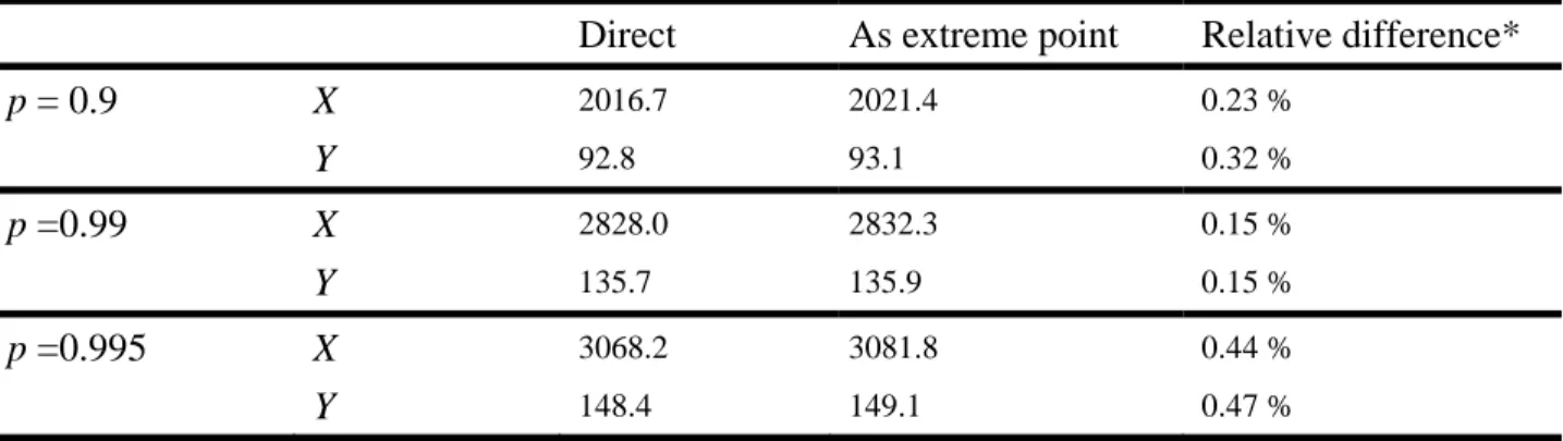
each site, similarity is observed between the estimation errors of the univariate quantiles evaluated both directly and as extreme scenarios even when only one sample is considered. Note that similar errors do not imply similar estimated values. Table 2 presents the true values of the univariate quantiles evaluated directly and as extreme scenarios of the bivariate curve. Table 2 provides also an indication about the relative difference between the two estimates. These relative differences are very low (less than 0.5%). Therefore, one can consider that values obtained by the two different methods are almost the same.

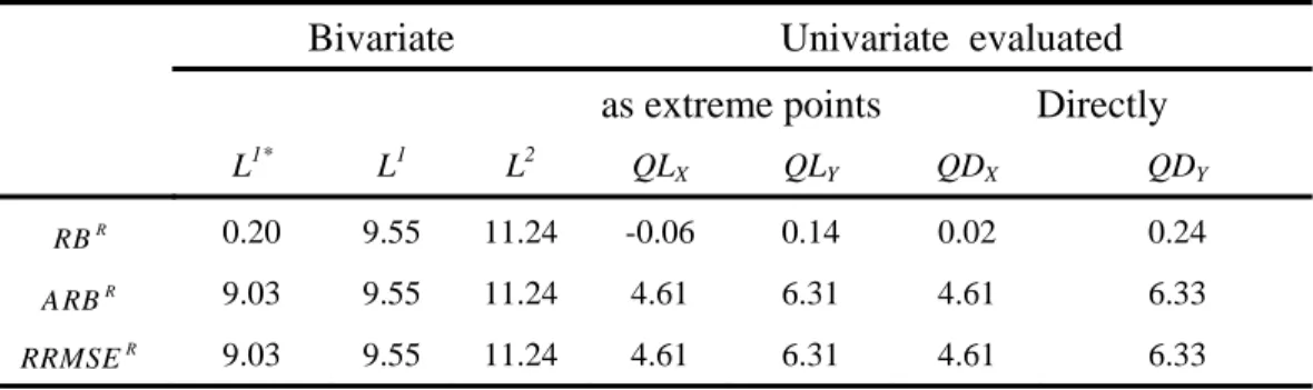
The second preliminary simulation results are presented in Table 3 which summarises the values of the criteria related to the same previously generated region for the bivariate as well as the univariate estimation. For the bivariate case we opted to present all possible combinations of criteria (RBR, ARBR and RRMSER) and “norms” (L1*, L1 and L2).. Note that the values in Table 3 represent the whole region while values in Table 1 represent only particular sites. Bivariate results show, as expected, that it is appropriate to use L1* for the RBR and ARBR evaluation and L1 for the RRMSER evaluation. The values associated to L2 are given only as an indication. Hence, and in order to save space in the remainder of the paper, they are omitted. Furthermore, the regional averages of the univariate quantile errors estimated directly or as extreme scenarios are similar. Figures 3b,c show the true and estimated quantile curves, respectively, for all sites of the generated region. It can be seen that the true quantile curves are well ordered whereas the estimated ones intersect. This is because in the first case the parameters are known and ordered whereas in the second case the parameters are estimated and do not necessarily keep their order. Nevertheless, the whole view of the region, composed by the two groups of curves (true and estimated), shows a good agreement as a region and not for each site alone. The curves in Figures

3b,c are also in agreement with the values corresponding to L1* in Table 3. The agreement here concerns the whole region (all sites together) rather than site by site.

As it was previously indicated, univariate quantiles can be either estimated directly using the index-flood model or deduced from the bivariate estimation as extreme scenarios (extreme points of the quantile curve). Hence, in this third preliminary simulation, it is valuable to compare univariate quantiles obtained from both estimations. Table 4 shows, on the basis of M = 2000 generated HetMa50 regions with p = 0.9, 0.99 and 0.995, relative errors corresponding to univariate quantile estimation. These results combined to those in Table 2 indicate that, for a given variable X or Y, directly evaluated quantile estimates are very similar to those obtained as extreme points of the bivariate quantile curves for all values of p and for each criterion. This result remains valid for the outputs of the main simulations. Consequently, results related to the univariate quantiles when evaluated as extreme points are omitted from the next simulation results. This result shows that values provided by multivariate FA are very similar to those obtained by the univariate FA and also with an equivalent accuracy.

5.2 Main results

The main simulation results are presented in Tables 5a,b for all the considered regions. Even though, the focus is on quantile curve estimation, the evaluation of growth curve estimation qC _p is also reported in order to explain the quantile results. From both tables, three apparent elements can be observed:

- In general, the values of the performance criteria increase with respect to the risk p in both univariate and bivariate settings. This behaviour, well known in the univariate FA, is not

systematic in the bivariate estimation, especially in terms of RRMSER. The usual explanation is that generally in FA, a quantile associated to a risk p is more accurately estimated than another one associated to a risk p′ if p < p′ (when p and p′ are close to 1). The reason is that for a small risk, the corresponding quantile is close to the central body of the distribution, and hence, an important part of the data contributes to its estimation. However, in the bivariate setting, the situation is not similar. Indeed, in the multivariate context, the central part of a distribution contains little probability mass compared to the univariate setting. This is very obvious in higher dimensions; see Scott (1992) for more details and examples.

- The relative bias RBR is very small in all regions and for all values of p. However, bivariate RBR’s are larger than those of each one of the univariate but without exceeding 1.17%. The RBR low values are due to the symmetry regarding the parameters of the simulated regions. - The growth curve qC results, for each value of p, are very similar for both variables _p

separately (univariate) and also jointly (bivariate), especially in terms of RRMSER. However, this is not the case for quantile QC estimation where differences are noticeable between _p bivariate and univariate results. This can be explained by the errors induced from the estimation of the index μ. That is, if one variable has a high error in its index μ, then, when multiplying it by the growth curve qC , the final estimation result is affected accordingly. _p Note that the uncertainty related to the mean has more effect on the variability of the quantiles (through the RRMSER) than on the bias (RBR) because of error compensation in the RBR.

In the homogeneous regions (Table 5a), the variability expressed in terms of the RRMSER in the growth curve estimation qC is small compared to that of _p QC for a fixed p. Hence, in _p

homogeneous regions, the variability in QC estimation originates essentially from the _p estimation of the index μ in equations (1) and (6). However, with respect to p, the variability in

p

qC estimation increases faster than the variability in QC . This result may be explained by the _p

fact that the mean has more influence on the central part of the distribution than on the tail. Hence, the contribution of the index variability decreases for large values of p.

Table 5b presents results of Homog and HetMa50 when the variables X and Y are assumed to be independent, that is γ = 1 in copula (8). From Tables 5a,b, the comparison of the dependent and independent cases reveals two principal elements. First, there is no significant difference in the univariate results: The results of univariate estimation quantiles remain almost the same in both dependent and independent cases. The reason is that, intuitively, the marginal distributions are not affected by the copula, and mathematically, the copula has always the same values in the extreme points, that is C(u, 1) = u and C(1,v) = v for all u, v in [0,1] (see e.g. Nelsen, 2006). Second, in bivariate quantile estimation, the criteria values are slightly smaller in the independent case than in the dependent one. This may be justified by the presence of an extra parameter to be estimated in the dependent case (the parameter γ ). This parameter in the independent case is not estimated and is fixed at γ = 1. We conclude that univariate estimation ignores the dependence structure of the event.

Figure 4 shows the quantile estimation performance with respect to the 15 sites within the same simulated regions HetMa50 presented in Table 5a. The Bi and Ri, defined in (15), represent respectively the RB and the RRMSE for a site i. Similar results are obtained for the other types of regions and hence they are omitted. From Figure 4 the behaviours of both the RB and the RRMSE, obtained from the bivariate or univariate models are similar. It is observed that for each

value of p, the bias is positive for the first half of the sites (from the 1st to the 8th site) and negative for the other half (from the 9th to the 15th site). This fact is observed in the univariate setting as well as in the bivariate one. It may be explained as follows: In the first half, the true quantile Q is smaller than the average quantile over the region Q , Q ≤ , since small values of Q the scale parameter α reduce quantile values in regions like HetMa50. Furthermore, the average quantile value should be very close to the estimated one ˆQ (Q ≈ ). Therefore, the quantile Qˆ relative error is positive since it is greater than the negligible difference error between the estimate and the average quantiles ( ˆQ − ≥ − ≈ ). The other half of the sites, where the Q Qˆ Q 0 bias is negative, can be treated similarly. Furthermore, we note that the RRMSE is small for sites with parameters close to those of the homogeneous region given in (9) and it increases according to the deviation of the site parameters from the central one. This is more apparent for high values of p. This behaviour of the RB and RRMSE with respect to site number is also observed in the univariate index-flood model (Hosking and Wallis, 1997).

5.3 Effect of various factors on the estimation results

The proposed estimation model (6) may be affected by several factors. In this section, we present a short study dealing with the impact of the record length n, the region size N as well as the degree of region heterogeneity. Table 6 presents estimation results for the Homog, HetCo30 and HetMa50 regions when the variables are dependent where N = 15 and n = 30, 60 and 100. To facilitate comparisons, results for n = 30 are taken from Table 5a. We observe that when n increases, the main improvement is related to the RRMSER for each value of p. However, the RBR and the ARBR remain almost constant. Note that the values of the RBR and the ARBR are very low and their variations can be considered as proportionally similar to those of the RRMSER. On the

one hand, the improvement of the RRMSER, with respect to n, is related to the heterogeneity degree of the region. That is, the improvement decreases slightly from Homog to HetMa50. On the other hand, the improvement for the bivariate estimation is slightly more important than for the univariate estimation in all considered regions.

Similarly to Table 6, Table 7 presents estimation results of 0.99-quantiles for Homog, HetCo30 and HetMa50 regions when the variables are dependent where n = 30 and N = 10, 15, 20, 50 and 100. In order to simplify the comparison, results for N = 15 are taken from Table 5a. We observe, for a given type of region, a very slight improvement (less than 1%) of the RRMSER in both univariate and bivariate estimations whereas the RBR and the ARBR are almost constant but with a variability proportionally similar to the variability of the RRMSER. This behaviour with respect to N is similar for the three region types although the values are different. The results corresponding to the 0.9- and 0.995-quantiles lead to similar conclusions and hence are not presented.

An important assumption of RFA (and the Index-flood model) is the homogeneity of the region which is checked in the delineation step. To study the effect of the heterogeneity degree of a region, we consider five regions with different heterogeneity degrees: one homogeneous region, two possibly homogeneous regions and two heterogeneous regions. The corresponding results are presented in Table 8. They indicate that, for each fixed value of p in the univariate as well as the bivariate settings, the quantile and the growth curve estimation errors increase with respect to the heterogeneity degree expressed through the mean values of H. It can be concluded that the heterogeneity degree has a negative effect on the performance of the estimation procedure.

We conclude from Tables 6 and 7 that the impact of n and N is not significant on regional quantile estimation. Note that, in the hydrological context, the variations of n and N are generally

small. However, as concluded in Chebana and Ouarda (2007), the effect of n and N is very important in the delineation step. Hence, the impact of the record length n and the region size N is indirect on the estimation step through the homogeneous region selection in the delineation step. Even though the estimation is not greatly affected by increasing values of N, there is still significant gain for carrying out the regionalisation (transfer of information from other sites in the region). Indeed, when N = 1, if the target-site contains enough data, then quantile estimation can be obtained directly by local FA. The regional methodology is of interest when the target-site is ungauged or partially ungauged so that the local estimation is not possible or not efficient. The homogeneity or the possible homogeneity of regions are important conditions to the good performance of the procedure. The above conclusions are similar to those obtained by Hosking and Wallis (1997) for the univariate model.

In the previous results, univariate and bivariate estimates were shown to be different in terms of values but similar in terms of behaviour. The explanation lies partially in the difference in the criteria employed to evaluate the performances of each model. Furthermore, the main differences between univariate and bivariate models are conceptual. The univariate estimation results are presented only to be compared to the extreme points of the bivariate quantiles.

6 CONCLUSIONS AND FUTURE WORK

In the present paper we proposed an extension of the index-flood model to the multivariate context. The proposed estimation procedure with the multivariate discordancy and homogeneity tests constitute a complete multivariate RFA procedure. Even though the procedure is shown to be valid in the multivariate setting, the present paper focuses on the bivariate case. The proposed model is based on copulas and on a bivariate quantile version. The bivariate quantile version employed is a curve composed by several statistically similar combinations, since they lead to the same risk. The univariate estimated quantiles, correctly combined, are particular cases corresponding to the extreme scenarios of the bivariate quantile curve. According to the available resources and the nature of the project, one or more convenient scenarios may be selected. Hence, the bivariate setting offers more flexibility to designers than the univariate framework.

Simulation results of the bivariate version of the index-flood model are similar to those of the univariate model in terms of behaviour of the corresponding performance criteria. The results of univariate FA are provided (as extreme points) by the multivariate FA, and with an equivalent accuracy. The proposed model performs better when the region is close to homogeneity. Its performance is not significantly affected by small variations of the record length of sites or the region size. However, the whole regionalization procedure is affected by these factors through the delineation step. On the other hand, the univariate estimation results remain almost unchanged if the variables are dependent or independent. Hence, the univariate quantile estimates do not take into account the dependence structure of the variables characterizing the event.

In the present study several elements of multivariate RFA are treated. Nevertheless, the following issues, among others, should have the merit to be developed in future efforts:

- Adaptation of the model for the estimation of other events of interest such as the simultaneous exceedence event expressed as

{

X ≥x Y, ≥ y

}

,

- Estimation of the multivariate index-flood μ for ungauged sites using their physiographical characteristics,

- Definition of sharp criteria to measure the model performances. Indeed, if other phenomena and other types of copula are considered, then “distances” will be between sets instead of functions, since generally a quantile curve is a “set of points” and not necessarily a function (which is a particular case),

- Development of confidence bands associated to the regional estimates of the quantile curves. This is of interest to evaluate the amount of variation in the curve estimation. - A thorough sensitivity study of the impact of different factors that may affect the

performances of the model, separately or combined. Such factors include: the estimation method of the distribution parameters, the fitted regional distribution including copula, as well as the effect of a misspecification of the bivariate distribution.

ACKNOWLEDGMENTS

Financial support for this study was graciously provided by the Natural Sciences and Engineering Research Council (NSERC) of Canada, and the Canada Research Chair Program. The authors wish to thank the Editor, Associate Editor and three anonymous reviewers whose comments helped improve the quality of the paper.

NOTATION LIST

, , ,

X X Y Y

α β α β _{Parameters of the marginal Gumbel distributions} γ _{Dependence parameter in the Gumbel logistic copula}

ρ _{Correlation coefficient}

τ _{Kendall tau coefficient} , _X and _Y

F F F Joint distribution and marginal distributions for the random variables X and Y (.,.)

C_γ Gumbel logistic copula with parameter γ D Bivariate discordancy test

H Bivariate homogeneity test n or n_i Site record length (of site i) N Number of sites in a region

M Number of replicates for the simulations p

QC Bivariate quantile curve associated to a risk p of the non-exceeding event

, ( )

x y

Q p A point (a combination) of the curve QC_p ( )

x

QC p and ( )QCy p

Coordinates of the point Q_{x y,} ( )p , that is Q_{x y,} ( )p =

(

QC p QC_x( ), _y( )p

)

( )

X

QD p

and ( )QD_Y p Univariate quantiles when directly evaluated ( )

X

QL p and ( )QL_Y p

Univariate quantiles when deduced as extreme values from the bivariate quantile curve

[ ],

(.)

m i p

R Coordinate-wise relative errors of the proper part of the quantile curve of site i corresponding to the replication m and for a risk p

i p

L Length of the proper part of the true quantile curve QCi_p of site i and for a risk p

*[ ]

( ) m i

RIE p Relative integrated error related to R[_pm i], (.)

[ ]

( ) m i

RIE p Relative integrated error related to Rp[m i], (.) ( )

i

B p Bias for a site i evaluated on the basis of RIE_i*[m]( )p ( )

i

R p Root-mean square error for a site i evaluated on the basis of RIEi[m]( )p ( )

R

RB p Regional bias evaluated as a mean over the region of B p _i( ) ( )

R

A RB p Regional absolute bias evaluated as a mean over the region of B pi( )

( ) R

RRMSE p Regional quadratic error evaluated as a mean over the region of R p _i( )

The notations employed for the quantile curve are valid for the growth curve quantile by replacing Q by q

BIBLIOGRAPHY

Abdous, B. and Theodorecu, R. (1992). Note on the spatial quantile of a random vector. Statist. Probab. Lett., 13, 333-336.

Adamowski, K. and Feluch, W. (1990). Nonparametric flood frequency analysis with historical information. ASCE J. Hydraul. Engng., 116, 1035–1047.

Alila, Y. (1999). A hierarchical approach for the regionalization of precipitation annual maxima in Canada. J. Geophys. Res., 104, 31,645-31,655.

Alila, Y. (2000) Regional rainfall depth-duration-frequency equations for Canada. Water Resour. Res., 36, 1767-1778.

Ashkar, F. (1980). Partial duration series models for flood analysis. PhD thesis, Ecole Polytechnique of Montreal, Montreal, Canada.

Belzunce, F., Castaño, A.; Olvera-Cervantes, A. and Suárez-Llorens A. (2007). Quantile curves and dependence structure for bivariate distributions. Comput. Statist. Data Anal., 51, Issue 10, 5112-5129.

Bocchiola, D., De Michele, C. and Rosso, R. (2003). Review of recent advances in index flood estimation. Hydrol. Earth Syst. Sci., 7, 283-296

Burn, D. H. (1990). Evaluation of regional flood frequency analysis with a region of influence approach. Water Resour. Res., 26, 2257-2265.

Chaudhuri, P. (1996). On a geometric notion of quantiles for multivariate data, J. Amer. Statist. Assoc., 91, 862-872.

Chebana, F. and Ouarda, T.B.M.J. (2007). Multivariate L-moment homogeneity test. Water Resour. Res., 43, W08406, doi:10.1029/2006WR005639.

Chebana, F.and Ouarda, T.B.M.J. (2008a). Depth and homogeneity in regional flood frequency analysis. Water Resour. Res., 44, W11422, doi:10.1029/2007WR006771.

Chebana, F. and Ouarda, T.B.M.J. (2008b). Multivariate quantiles in hydrological frequency analysis. Research report, R-1021. INRS-ETE, Québec, Canada. 47 pp.

Cunnane, C. (1978). Unbiased plotting positions—a review. J. Hydrology, 37, 205–222.

Dalrymple, T. (1960). Flood frequency methods. United States Geological Survey Water-Supply Paper, 1543 A, 11-51.

De Michele, C., Salvadori, G., Canossi, M., Petaccia, A. and Rosso, R. (2005). Bivariate Statistical Approach to Check Adequacy of Dam Spillway. J. Hydrologic Engrg., 10, 50-57. Durrans, S.R. and Tomic, S. (1996). Regionalization of low-flow frequency estimates: an

Alabama case study. Water Resour. Bull., 32, 23-37.

Einmahl, J. H. J. and Mason, D. M. (1992). Generalized quantile processes. Ann. Statist., 20, 1062-1078.

Fermanian, J-D. (2005). Goodness-of-fit tests for copulas.J. Multivariate Anal., 95, 119-152. Genest, C. and Rivest, L-P. (1993). Statistical Inference Procedures for Bivariate Archimedean

Copulas.J. Amer. Statist. Assoc., 88, 1034-1043.

Genest, C., Rémillard, B. and Beaudoin, D. (2009). Goodness-of-fit tests for copulas: A review and a power study. Insurance: Mathematics and Economics, 44, In Press.

Ghoudi, K., Khoudraji, A. and Rivest, L-P. (1998). Propriétés statistiques des copules de valeurs extrêmes bidimensionnelles. Canad. J. Statist., 26, 87-197.

GREHYS (1996a). Presentation and review of some methods for regional flood frequency analysis. J. Hydrology, 186, 63-84.

GREHYS (1996b). Inter-comparison of regional flood frequency procedures for Canadian rivers. J. Hydrology, 186, 85-103.

Gumbel, E.J. and Mustafi, C.K. (1967). Some analytical properties of bivariate extreme distributions. J. Amer. Statist. Assoc., 62, 569–588.

Hamza, A., Ouarda, T.B.M.J., Durrans, R. S. and B. Bobée (2001). Development of scale invariance and tail models for the regional estimation of low-flows. [French] Can. J. Civ. Eng., 28, 291—304.

Hettmansperger T. P., Nyblom, J. and Oja, H. (1992). On multivariate notions of sign and rank, in: Y. DODGE (ed.), L1-Statistical analysis and related methods, North-Holland, Amsterdam, 267–278.

Hosking, J. R. M. and Wallis, J. R. (1993). Some statistics useful in regional frequency analysis. Water Resour. Res., 29, 271-282.

Hosking, J. R. M. and Wallis, J. R. (1997). Regional Frequency Analysis: An Approach Based on L-Moments. Cambridge University Press. 240 pages.

Jones, F. (1993). Lebesgue integration on Euclidean space. Jones and Bartlett Publishers, Boston, MA, 588 pages.