HAL Id: hal-00757189
https://hal-agrocampus-ouest.archives-ouvertes.fr/hal-00757189
Submitted on 26 Nov 2012
HAL is a multi-disciplinary open access
archive for the deposit and dissemination of
sci-entific research documents, whether they are
pub-lished or not. The documents may come from
teaching and research institutions in France or
abroad, or from public or private research centers.
L’archive ouverte pluridisciplinaire HAL, est
destinée au dépôt et à la diffusion de documents
scientifiques de niveau recherche, publiés ou non,
émanant des établissements d’enseignement et de
recherche français ou étrangers, des laboratoires
publics ou privés.
Cognitive Maps and Bayesian Networks for Knowledge
Representation and Reasoning
Karima Sedki, Louis Bonneau de Beaufort
To cite this version:
Karima Sedki, Louis Bonneau de Beaufort. Cognitive Maps and Bayesian Networks for Knowledge
Representation and Reasoning. 24th International Conference on Tools with Artificial Intelligence,
2012, Greece. pp.1035-1040, �10.1109/ICTAI.2012.175�. �hal-00757189�
Cognitive Maps and Bayesian Networks for
Knowledge Representation and Reasoning
Karima Sedki
1. AGROCAMPUS OUEST, UMR6074 IRISA, F-35042 Rennes, France 2. Université européenne de Bretagne, France
Email: [email protected]
Louis Bonneau de Beaufort
1. AGROCAMPUS OUEST, UMR6074 IRISA, F-35042 Rennes, France 2. Université européenne de Bretagne, France
Email: [email protected]
Abstract—Cognitive maps are powerful graphical models for knowledge representation. They offer an easy means to express individual’s judgments, thinking or beliefs about a given problem. However, drawing inferences in cognitive maps, especially when the problem is complex, may not be an easy task. The main reason of this limitation in cognitive maps is that they do not model uncertainty with the variables. Our contribution in this paper is twofold : we firstly enrich the cognitive map formalism regarding the influence relation and then we propose to built a Bayesian causal map (BCM) from the constructed cognitive map in order to lead reasoning on the problem. A simple application on a real problem is given, it concerns fishing activities.
I. INTRODUCTION
To solve a given decision problem, there is often need to firstly provide knowledge and judgment analysis of the problem. This task is not easy, especially when the elicitation process includes several domain experts where each one has his own view of the problem. The difficulty appears namely in used variables (factors, events, etc.), the type of relationships between variables (dependencies, causality, correlation, etc.), the nature of data (uncertain, incomplete, etc.), etc. So, it is important to choose a model that allows to respond to the targeted objective. Graphical Models, such as cognitive maps (CMs) [5], Bayesian networks (BNs) [6], are powerful models for representing domain knowledge. They have been widely used for solving various problems [3], [2], [7].
In this paper, the studied problem concerns the analysis of shells fishing activity in the west region of France (rade de Brest). The objective consists to study the views of fishermen about their activity. Namely, the goal is to determine the variables or factors that may impact fishermen in their activity and environment (for example, analyze the impact of environmental conditions, material and human means in the fishing activity). We first use a cognitive map (CM) formalism to represent the perception of the interviewed actors. CM is a directed graph which represents variables and causal relations between the variables in a decision problem. They have the advantage to describe and capture the decision makers knowledge in a more comprehensive and less time-consuming manner than other methods [11].
As we mentioned above, the elicitation step is important for solving and modeling decision problems. However, another important step is also required. It concerns inference process which consists in obtaining new facts or conclusions from other information. However, drawing inferences in CMs, especially when the problem is complex, may not be an easy task [9]. The first reason of this limitation in CMs is that they do not model uncertainty with the variables. In addition, the variables in cognitive maps are represented in a static way. Namely, the way in which the beliefs of decision-makers about some target variables change when they learn additional information about the concepts of the map is not represented. In the other hand, although BNs are a well-established method for reasoning under uncertainty and making inferences, the elicitation of the structure and parameters of the network in complex domains can be a tedious and time-consuming task. Moreover, the notion of probability is often not perceived or understood by domain experts. The task is therefore more tedious and time-consuming for generating conditional probabilities.
It is clear that in our problem, using the cognitive map model is not sufficient to analyze and understand the impact of the different variables of the problem and using the Bayesian network (BN) for generating the conditional probabilities from fishermen is not also an easy task. However, despite the limitations of each model (BN and CM), combining them is possible. The combined model is called Bayesian causal map (BCM) [10]. To construct a BCM, the procedure consists firstly in constructing a cognitive map and then convert it into a Bayesian causal map. In [10], the authors use the initial CM only to construct the structure of the BCM. They define the parameters (local probabilities) of the BCM from experts knowledge. This means that domain experts are in a first step solicited for the construction of the CM and second in the definition of the conditional probabilities.
In this paper, our proposition consists firstly in an extension of the CM formalism by enriching the causal relation with additional information (for example, information about the influence of each causal concept when the premise variable
increases and decreases). Secondly, we propose to transform the constructed CM into BCM. Concerning the structure of the BCM, we follow the procedure described in [10]. Concerning the parameters of the BCM, we propose to take into account the causal values associated to the relations of the constructed CM. Namely, the elicitation step of the BCM will be less tedious since the structure and the parameters of the BCM are defined from the constructed CM. Finally, we propose to built a BCM in order to analyze the problem of shells fishing activity. The CM is constructed from judgments and beliefs of several actors (fishermen) and then we transform it into a BCM following the proposed approach.
The rest of the paper is organized as follows: In section II, we present some important issues related to BNs and CMs. In Section III, we present the new CM formalism. Section IV proposes a procedure to construct a Bayesian causal map. Section V presents the studied problem with some simulation cases. Section VI concludes the paper.
II. COGNITIVE MAPS ANDBAYESIAN NETWORKS
In this section, we provide a brief description of cognitive maps and Bayesian networks.
A. Cognitive maps
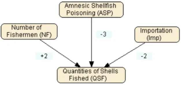
A cognitive map, also called causal map, is a directed graph that represents the knowledge of decision makers. It expresses individual’s judgments, thinking or beliefs about a given problem [5], [1]. Figure 1 gives an example of a CM.
Fig. 1. A simple example of cognitive map.
We distinguish three principal components in a CM 1) Concepts: A node in a cognitive map represents a
concept which corresponds to a variable (attributes, factors or events) of the studied problem.
2) Causal relations: An arc between two concepts in a cognitive map represents a causal relation. It depicts a cause-effect (or cause-consequence) relation between two concepts. If we have a causal relation from concept Atowards a concept B, then A is called a causal concept and B is called an effect concept. We distinguish two forms of causal relations:
a) A positive relation between two concepts indicates that an increase in the causal concept leads to an increase in the effect concept.
b) A negative relation indicates that an increase in the causal concept leads to a decrease in the effect concept or decrease in the causal concept leads to increase in the effect concept.
For example, in Figure 1, a causal relation between Number of fishermen (NF) and Quantities of shells fished (QSF) is positive which denotes that the higher the NF, the higher will be the QSF. On the other hand, the causal relation between the concept Importation (Imp) and Quantities of shells fished is negative, it establishes that the higher the Imp, the lower the QSF. 3) Causal values: Each positive or negative relation can
be associated with a numerical value, called a causal value. It represents the strength of the causal relation. When the continuous values of the CM are in the interval [−1, +1], they represent fuzzy cognitive maps [8]. In this paper, the considered causal value can be Low (−1 or +1) (resp. M edium (−2 or +2 ), High (−3,+3), N ull (0)). These values are used in drawing CMs since this is easier and more intuitive for elicitation. CM allows only deductive reasoning (predicting an effect given a cause). Thus, we can get responses about the effects of a given cause but we can’t answer why effects are produced. B. Bayesian Networks
Bayesian networks [6] are widely used in decision making mainly for problems that contain uncertain information. They are probabilistic models specified by two components:
1) A qualitative component: It represents independence relations by a directed acyclic graph (DAG), where each node xi represents a variable, and arcs represent the
corresponding relationships between these variables. 2) A quantitative component: It quantifies the uncertainty
of the relationships between variables. Each variable contains the states of the event that it represents and a conditional probability table (CP T ). The CP T of a variable contains probabilities of the variable being in a specific state given the states of its parents. The joint probability distribution for X = {x1, x2, ..., xn} is given
by the chain rule :
P (x1, x2, ..., xn) =
Y
i=1...n
P (Xi|P ai) (1)
where P ai represents the parents of xi.
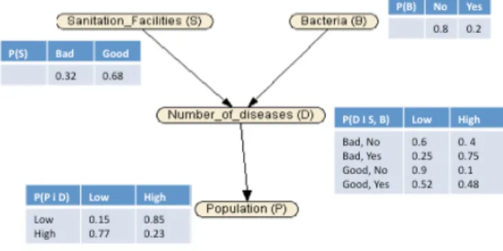
In Figure 2, we have an example of a BN which contains four variables (B, S, D and P ). B has two states (No, Yes) and has no parents. S and B are two parents of D which is a parent of P . For each variable, there is need to specify a conditional probability distribution table. In Figure 2, we observe these tables: P(B), P(S), P(D | S, B) and P(P | D). In Figure 2, there is no arc between the variables B and S, so these two variables are independent; there is arc from B and S to D, this denotes that D is dependent of B and S. There is also
no arc between B and P and no arc between S and P , this means that P is conditionally independent of B and S given D (conditional independence assumption in BNs).
Fig. 2. An example of Bayesian Network.
Another important notion in BN is the one of probabilistic inference. It allows to compute the probability of any variable given some observed variables. Inference in BN is based on the notion of propagating evidence. We can use BN to perform abductive reasoning (diagnosing a cause given an effect) and deductive reasoning (predicting an effect given a cause).
III. THE NEW FORMALISM OF COGNITIVE MAP
In the original cognitive map formalism, each positive or negative relation is assigned with only one value which can be positive or negative. The causal relation is symmetric, this means that an increase of the causal concept has symmetric impact on the effect concept than decreasing of the same causal concept. For example, in case where the causal relation between two concepts x and y is negative, if an increase of the causal concept x causes high decreasing in the effect concept y, then decreasing of x causes high increasing of y. In the example of Figure 1, increasing of ASP causes high decreasing of QSF (-3). The influence of decreasing of ASP is supposed to be symmetric, namely it causes high increasing of QSF (+3) which is not correspond to judgment of fishermen. In this paper, we propose to enrich the formalism by assigning two values to each causal relation. Namely, the new formalism informs us about the impact of increasing and decreasing of the causal concept which is not necessarily symmetric. So, in the new formalism:
• Each causal relation is assigned two values represented by [V1, V2].
• V1 represents the influence degree on the effect concept
when the causal concept increases.
• V2 represents the influence degree on the effect concept
when the causal concept decreases.
• V1 and V2 are numerical values, each one can be either
positive, negative or null. Each of V1and V2can be Low
(−1 or +1) (resp. M edium (−2 or +2 ), High (−3,+3), N ull (0).
• V1is positive if the increase of the causal concept causes
increasing in the effect concept.
• V1 is negative if increasing the causal concept causes
decreasing in the effect concept.
• V1is null if increasing the causal concept has no impact
on the effect concept.
• V2 is positive if decreasing the causal concept causes
increasing in the effect concept.
• V2 is negative if decreasing the causal concept causes
decreasing in the effect concept.
• V2is null if decreasing the causal concept has no impact
on the effect concept.
The difference between the new formalism and the original one is that the causal relation is not necessarily symmetric in the extended formalism. For example, in the new formalism, if increasing the causal concept leads to increasing in the effect concept (suppose that the impact is high), then decreasing of the causal concept can lead to increasing or decreasing the effect concept (the impact can be low, medium or high), the influence on the effect concept can have also no impact on the effect concept. An example of the new formalism is given in Figure 3.
Fig. 3. An example of the new cognitive map formalism.
The information [+2, −3] between the causal concept N umber of f ishermen (N F ) and the effect concept Quantities of shells f ished (QSF ) means that an increase of N F causes an increase of QSF (+2) and decreasing of N F causes a decrease of QSF (−3). The information [−3, 0] between the causal concept ASP and the effect concept QSF means that an increase of ASP causes a decrease of QSF (−3) and decreasing of ASP has no impact on QSF (0) (while in the original formalism as observed in Figure 1 increasing of ASP causes decreasing of QSF (−3) and decreasing of ASP causes increasing of QSF (as the relation is symmetric, the value is by default equal to +3)).
IV. FROM A COGNITIVE MAP INTOA BAYESIAN CAUSAL MAP
As mentioned previously, CMs have the advantage to describe and capture the decision makers knowledge in a comprehensive manner, hence the modeling is closer to natural language. However their limitation is that they do not model uncertainty with variables. So, they allow only limited forms of causal inferences. On the other hand, defining the conditional
probabilities in BNs from experts is not an easy task, especially when the domain of variables is large. Thus, in order to reduce the complexity of the elicitation step to solve a decision problem and make inferences in the model, we propose to use the new cognitive map formalism for the elicitation step and to transform it into a Bayesian causal map (BCM) for the reasoning step. To construct the BCM, the procedure is the following:
1) Derive the CM of the concerned problem. In the studied problem, the CM is derived from the judgments and beliefs of several actors (fishermen) following the new formalism.
2) Construct the structure (Qualitative component) of the BCM which should be a directed acyclic graph (DAG). As the semantic of the arcs in the two models is the same, the structure of the BCM is based on the constructed cognitive map.
3) Define the associated parameters (Quantitative compo-nent) which correspond to probability distributions. This step requires some operations in order to capture the semantic of causal values.
We describe the procedure to construct the structure and parameters of the BCM in the following two subsections. A. Construction of the structure of the BCM
The structure of the BCM describes the relationships between the variables of the problem. It is represented by a DAG. As we construct the BCM from a cognitive map, its structure corresponds to the structure of the CM with some modifications. The authors in [10] proposed a procedure to obtain the structure of the BCM from a cognitive map. This procedure concerns particularly the following points:
1) Conditional independencies: In a CM, the existence of a relation between two variables induces that these variables are dependent. However, the absence of a relation between two variables does not imply independence (i.e., lack of dependence) between these two variables. In BN, the absence of a relation between variables induces that some variables are conditionally independent on other variables. If we have a sequence of variables, an absence of an arrow from a variable to its successors in the sequence implies conditional independence between the variables. Thus, when defining the structure of the BCM from the constructed CM, it is important to ensure the nature of relations between variables of the studied decision problem because this allows to specify the relevant information in making inferences.
2) Direct and indirect relationships: Generally, experts draw direct links between concepts even if they are influenced through another concept. Namely, they take into account the fact that the concepts are linked but not how (this is also observed in our problem where
fishermen use often direct links). In BN, a relationship between variables is direct if they are directly linked with an arrow and is indirect if the variables are conditionally independent. So, distinguishing between direct and indirect relationships is important namely in order to determine the conditional independencies between variables of the problem. If a given variable affects a second variable only through a third variable, then an arrow from the first variable to the second is redundant and increases the complexity of the representation.
3) Circular relations: Contrary to BNs, which are acyclic graphs, in a CM, the relations can be circular. The existence of circular relations can be due to two main reasons [4], [11]. First, they may represent mistakes that need to be corrected (in this case, users are reasoning deductively, i.e. from causal to effect concepts and abductively on some concepts, i.e. form effects to causal concepts). Second, they may represent a dynamic structure of the map. Namely, they represent dynamic relations between variables over time. The solution in such cases consists to separate the variables into two different time frames. Namely, some relations in the cycle (or loop) belong to the present time frame while others belong to a future time frame [11].
In Section V, we give some examples concerning theses elements when we define the structure of the BCM of the case study.
B. Constructing the parameters of the BCM (generating CPT) Once the structure of the BCM is defined, we have to build the conditional probabilities tables (CPT) associated for each variable. In [11], the authors ask experts about the elicitation of the CPTs. They do not consider the causal values of the CM and therefore requires another elicitation step from experts. In this paper, we propose to take advantage of the causal values in the CM to generate directly the probabilities of the BCM. Avoiding a time consuming and tedious work especially as the notion of probability may be not intuitive of understand.
Deriving the conditional probabilities tables from causal values requires some operations in order to keep the semantic of these later on the one hand and to respect the conditions of probability theory on the other hand. Assume that Z is an effect concept and X, Y are the causes ones, i.e., X and Y are the parents of Z. When defining the CPT of the BCM, the semantic of the causal values should be preserved. For example if the positive effect of parents of Z is greater than the negative one, this should be traduced as P (Z = + | X, Y )> P (Z = − | X, Y ). The proposed procedure is described in the following:
1) Associate to each variable in the BCM its corresponding states: This consists in determining the domain of each variable. In our case, we consider that
each variable has two states (Decrease (−), Increase (+)). Theses two states allow to represent the negative or positive causal relation given in the constructed cognitive map. Namely, the objective in the BCM is to compute the probability that an effect variable (or child variable) increases or decreases given the cause variable (or parent variable) decreases or increases. 2) Associate a priori probabilities to variables without
parents: If we have informations about the problem, we can introduce them in the model and they will be represented as probabilities. In our case, as there is two states for each variable, the associated a priori probability for each state is 0.5 by default (there is no reason to specify another distribution). In addition, although we do not associate any distribution, there is no impact on the inference process since regarding theses variables, we can introduce any observations. 3) Building CPT for variables having parents: In our
method, causal values of the cognitive map are elicited from the experts. Thus, we directly use these values to obtain the CPT. The procedure is described in the following:
Let x a variable for which we compute the CPT and let yijthe parents of x. For each configuration (for example,
the variable having 3 parents, the corresponding CPT contains 8 configurations):
• yi− : are parents with a negative effect. E−
corre-sponds to the sum of the negative effects concerning yi−.
• yj+ : are parents with a positive effect. E+
corresponds to the sum of positive effects concerning yj+.
To compute P (x | yij), we define P (x = − | yij) and
P (x = + | yij).
For each configuration, if |E−|>|E+| (resp. if
|E+|>|E−|) then P (x=−|yij) > P (x=+|yij) (resp.
P (x=+|yij) > P (x=−|yij)). This means that
P (x=+|yij)=α*P (x=−|yij) with α = |E+| / |E−|
(resp. P (x=−|yij) = α*P (x=+|yij) with
α = |E−| / |E+|), 0<=α <=1.
Applying the condition of sum of probabilities is equal to 1, we have: P (x=−|yi−) + P (x=+|yj+)=1.
Hence P (x=−|yij)+α*P (x=−|yij)=1 (resp.
P (x=+|yij)+α*P (x=+|yij)=1 ). Then
• P (x=−|yij)=1/(1+α)
(resp. P (x=+|yij)=1/(1+α)) • P (x=+|yij) =1−P (x=−|yij)
(resp. P (x=−|yij) =1−P (x=+|yij))
Example 1: Let us consider the cognitive map of Figure 1 where the variable QSF has three parents (ASP , Imp and N F ). The aim is to generate CPT of QSF regarding its parent variables. Namely, we have to compute the probability that QSF increases or decreases given the 8 possible configurations of ASP , Imp, and N F (for example, the configuration where ASP , Imp, N F all increase or all decrease).
We illustrate the calcul with the configuration ASP , Imp and N F all increase. So, we have to compute P (QSF |ASP =+, Imp=+, N F =+). Namely, we compute P (QSF =+|ASP =+, Imp=+, N F =+) and P (QSF =−|ASP =+, Imp=+, N F =+).
Concerning this configuration (i.e. ASP , Imp and N F all increase), we have yi− = (ASP , IM P ) and yj+ =
(N F ). So, E− = -3 +-2 = -5 and E+ = +2.
We obtain | E− | > | E+ |, hence P (QSF = −
|ASP =+, Imp=+, N F =+) > P (QSF = + |ASP =+, Imp=+, N F =+) and α = 2/5 = 0.4. P (QSF = - | ASP = +, Imp = +, N F = +) = 1/(1+0.4) = 0.71 and
P (QSF = + | ASP = +, Imp = +, N F = +) = 1-0.71=0.29.
The results concerning the CP T of variable QSF concerning the 8 configurations are given in Table I.
ASP Imp NF P(QSF =+ ) P(QSF = - ) - - - 0.4 0.6 - - + 1 0 - + - 0 1 - + + 0.5 0.5 + - - 0.25 0.75 + - + 0.57 0.43 + + - 0 1 + + + 0.29 0. 71 TABLE I
THECPTOF THE VARIABLEQSFREGARDING HIS PARENTS
V. THE CASE STUDY:SHELLS FISHING PROBLEM
In this section, we apply our approach on a real problem which concerns the shells fishing activities. We firstly give the constructed CM and then we transform it into a BCM following the proposed procedure.
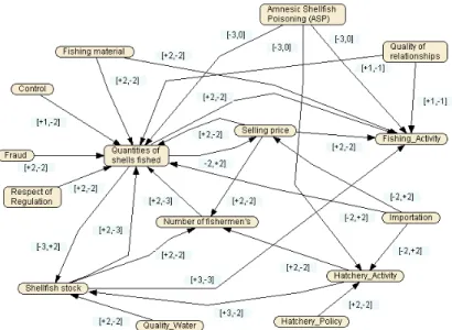
A. A cognitive map for the shells fishing problem In order to construct the CM, interviews are conducted with fishermen. These latter are asked to identify the concepts that might influence negatively or positively the fishing activities. The CM concerning this problem is given in Figure 4. The map contains 15 variables representing fishing activities (Shellfish stock (QSS), Quantities of fished shells (QSF), Hatchery Policy (HP), Hatchery Activity (HA)which appears to be an important
parameter for the dredging activity, Fishing Activity (FA)), environmental factors (Quality of Water), Fishing Conditions (Fishing Material, Quality of relationship between fishermen, Importation, Number of Fishermen, Control, Respect of Regulation) and other variables as Fraud, Selling Priceand the presence of a toxin called Amnesic Shellfish Poisoning (ASP) which influences negatively the fishing activity in general.
Fig. 4. The cognitive map for the shells fishing problem.
B. Construction of the BCM for the studied problem In order to analyze and study the impact of the variables on the fishing activities, the original map, shown in Figure 4, was used to construct a BCM. We first explain how the structure (i.e., the qualitative component) of the BCM is obtained and then we provide the final BCM with associated conditional probabilities tables to variables.
1) The structure of the BCM: As we observe in Figure 4, the constructed CM contains some circular relations, direct and indirect relations, etc. In order to construct a BCM from this CM, some relations are added and others are removed. We give here some examples of relations that are changed in the constructed BCM (Figures 5 and 6).
The first example of change concerns direct and indirect relationships between variables which implies that an arc between two variables in the network should represent a direct cause-effect relation only. Hence, in the constructed BCM, we consider that the variables Control, Fraud and Respect of Regulation do not have a direct effect on Quantities of fished shells. We modify this relation where Control has a direct effect on Fraud, which affects Respect of Regulation and then Quantities
of fished shells. In the original map, Importation affects directly Quantities of fished shells and there is also a direct link from Selling Price to Quantities of fished shells. In the modified cognitive map (see Figure 5), the relation between Importation and Quantities of fished shellsis indirect since the influence is obtained through Selling Price. Thus, the arrow from Importation to Quantities of fished shells is removed.
The second example of change concerns conditional independencies: in the constructed BCM (see Figures 5, 6), the arrow between Hatchery Activity and Number of Fishermen is removed. This implies that Hatchery Activityimpacts Number of Fishermen through Shellfish stock. Number of Fishermen is conditionally indepen-dent on Hatchery Activity given Quantities of shells in stock. If we have complete information about shellfish stock, any additional information on Hatchery Activity would be relevant in making inferences for Number of Fishermen. We have also the same change concerning the variable Quality of relationships where the arrow from this variable to Fishing Activity is removed because the influence between these two variables is presented through Quantities of fished shells. The arrow from ASP to Fishing Activity is also removed, they are considered as conditionally independent variables given Quantities of fished shells.
Another example of change concerns circular relations where a new concept (Shellfish stock (t+1)) was added to the constructed BCM in order to solve the problem of circularity and represent the dynamic relations between the variables across time frames. The dynamic relation is represented from Shellfish stock (t) to Quantities of fished shells and then to Shellfish stock (t+1).
As we observe in the BCM of Figure 5, some variables are also added (Fishing conditions) in order to simplify generating the CPTs. But we point out that this do not change the result if these variables are not added. Once the map is modified and re-organized, the conditional probability tables have to be determined. The CPT were generated using the weight (negative or positive) of links in the CM by applying the procedure described in Subsection IV-B. We use Netica software [12] to construct the model, introduce the probabilities associated with each variable and make probabilistic inferences. Figures 5 and 6 show the constructed BCM with different observations for each case.
C. Some scenarios analysis
The objective of building the BCM consists firstly to evaluate the fishing activities by analyzing the state of some variables (for example Quantities of fished shells, Shellfish stock, Hatchery Activity) regarding
observations about some facts (for example Fishing conditions, existence or no of ASP, Importation, Quality of relationships between fishermen, etc.). And secondly to diagnose causes given an effect. For example, what are the factors that cause increase or decrease in Fishing Activity.
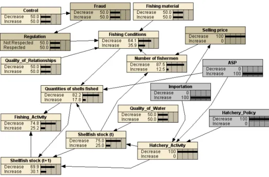
First scenario: Figure 5 shows the first scenario regarding some observations (variables on grey color). Applying propagation in the BCM, the probabilities of the rest of variables are updated.
Results of the first scenario show that when ASP and Importation increase and Hatchery Policy decreases, the probability that all the variables related to Fishing Activity(i.e., Quantities of fished shells (QFS), Fishing Activity (FA), Hatchery Activity (HA), shellfish stock (QSS(t) and QSS(t+1)) decreases is more than 0.5. Which explains the importance of these variables in the Fishing Activity. The obtained result in the BCM means that the impact concerning these observations is negative on some variables (the probability of each of the influenced variable decreases is more than 0.5) which is also represented in the original cognitive map (when ASP increases, the impact on some variables is negative (−3), when Imp increases, the impact is also negative (−2), and when HA decreases, the impact is also negative (−2)).
Second scenario: In the second scenario which concerns the diagnosing case. We introduce only one observation about the Fishing Activity where P (F ishing Activity=Decrease)=1. The probabilities of the rest of variables are updated (see Figure 6).
As it is shown in Figure 6, the probabilities associated to the state (Increase) of all the variables that influence negatively on most variables are greater than 0.5. And the probabilities associated to the state (decrease) of all the variables that influence positively on most variables are greater than 0.5. For example, when ASP increases, it influences negatively (-3) on Hatchery Activity and Quantity of shells fishing. After introducing observation about Fishing Activity, we obtain P (ASP = increase) >0.5, which confirms that the higher the ASP the lower the Quantity of fishing shells. This shows that the constructed BCM represents the initial judgments of the cognitive map, and it allows reasoning (diagnosis, inference).
Introducing different observation in the model regarding some variables as ASP, Importation, the model seems well established. We conclude that the proposed method is efficient, and this allows to analyze and understand the impact of the different variables.
VI. CONCLUSION
Solving a given decision problem using the CM or BN requires expert knowledge and judgements to determine the variables of the problem and influences between theses variables. However, using a CM to construct the model seems more natural than using BN because the modeling process consists only in providing the list of variables and the nature of influence (positive or negative). Using a BN requires more efforts from experts since they should take into account the uncertainty concerning the states of variables and the probabilistic nature of influences. Once the model is built even if we use the CM or BN, the objective is reasoning about the problem. BNs are a well established method and they offer efficient algorithm’s for applying inferences, learning and tools for the construction of the network. However, CMs present some limitations since they allow only some forms of inferences because of not modeling uncertainty. In order to facilitate of the modeling process and making inferences, we propose in this paper to take advantage benefits of the two models, i.e., BNs for the reasoning process and CMs for the elicitation process. We propose to firstly build the CM and then transform it into a BCM which combines causal modeling techniques and Bayesian probability theory. The structure of the obtained BCM corresponds to the one of the constructed CM from experts with some modification regarding the direct, indirect relations, circular relation and dependency between variables. The parameters of the BCM are obtained from the associated causal values in the CM.
We illustrated the proposed approach on a real decision problem which concerns the analysis of shells fishing problem. We conclude that using cognitive map is important because it allows to have the perception of fishermen. However, concerning the reasoning process, the BCM allows to analyze their perception. BCM also allows to revise the model in terms of variables, their influences and acquire some experience for elicitation. A future work concerns the fusion of cognitive maps because in our studied problem, several fishers can be interviewed about the same problem and each one has its own view about it.
REFERENCES
[1] B. Chaib-draa. Causal maps : Theory, implementation and practical applications in multiagent environments. In IEEE Transaction On Knowledge and Data Engineering, 2001. [2] Tina Comes, Michael Hiete, Niek Wijngaards, and Frank
Schult-mann. Decision maps: A framework for multi-criteria decision support under severe uncertainty. Decision Support Systems, 2011. doi:10.1016/j.dss.2011.05.008.
Fig. 5. The BCM concerning the first scenario for the shells fishing problem.
Fig. 6. The BCM concerning the second scenario for the shells fishing problem.
[3] Veronique Delcroix, Mohamed-Amine Maalej, and Sylvain Piechowiak. Bayesian networks versus other probabilistic mod-els for the multiple diagnosis of large devices. International Journal on Artificial Intelligence Tools, 16(3):417–433, 2007. [4] Ackermann F. Eden, C. Making Strategy. Sage Publications,
UK, 1998.
[5] Colin Eden and Steve Cropper. Cognitive mapping - a user’s guide. In Working paper, February 1990.
[6] Finn V. Jensen and Thomas D. Nielsen. Bayesian Networks and Decision Graphs. Springer Publishing Company, Incorporated, 2nd edition, 2007.
[7] D.F. Klein, J.H. Cooper. Cognition maps on decision workers in complex games. The Journal of the Operational Research Society, 33:63–71, 1982.
[8] Bart Kosko. Fuzzy cognitive maps. International Journal of Man-Machine Studies, 24(1):65–75, 1986.
[9] M. Laukkanen. Comparative cause mapping of organizational cognition. Meindl, J.R. Stubbart, C. Porac, J.F. Cognition Within and Between Organisations, pages 1–45, 1996.
[10] Shenoy P. Nadkarni, S. A bayesian network approach to making inferences in causal maps. European Journal of Operational Research, 128:479–498, 2001.
[11] Sucheta Nadkarni and Prakash P. Shenoy. A causal mapping approach to constructing bayesian networks. Decision Support Systems, 38:259–281, 2004.
[12] Norsys. Netica application, norsys software corp., http://www.norsys.com. 1998.