UNIVERSITÉ DE MONTRÉAL
WIDEBAND LINE/CABLE MODELS FOR REAL-TIME AND OFF-LINE
SIMULATIONS OF ELECTROMAGNETIC TRANSIENTS
OCTAVIO RAMOS LEANOS
DÉPARTEMENT DE GÉNIE ÉLECTRIQUE ÉCOLE POLYTECHNIQUE DE MONTRÉAL
THÈSE PRÉSENTÉE EN VUE DE L’OBTENTION DU DIPLÔME DE PHILOSOPHIAE DOCTOR
(GÉNIE ÉLECTRIQUE) AVRIL 2013
UNIVERSITÉ DE MONTRÉAL
ÉCOLE POLYTECHNIQUE DE MONTRÉAL
Cette thèse intitulée:
WIDEBAND LINE/CABLE MODELS FOR REAL-TIME AND OFF-LINE
SIMULATIONS OF ELECTROMAGNETIC TRANSIENTS
présentée par: RAMOS LEANOS Octavio
en vue de l’obtention du diplôme de : Philosophiae Doctor a été dûment accepté par le jury d’examen constitué de : M. KOCAR ILHAN, Ph.D., président
M. MAHSEREDJIAN JEAN, Ph.D., membre et directeur de recherche
M. NAREDO VILLAGRAN JOSE LUIS, Ph.D., membre et codirecteur de recherche M. DUFOUR CHRISTIAN, Ph.D., membre et codirecteur de recherche
M. MARTINEZ VELASCO JUAN A., Ph.D., membre M. GAGNON RICHARD, Ph.D., membre
DEDICATORY
AKNOWLEGMENTS
To my friend and advisor Jose Luis Naredo Villagran. Thank you for your patience, time and guidance.
To my advisor Jean Mahseredjian. Thank you for the opportunity and for letting me know that knowledge can be acquired from every situation.
To Christian Doufour. Thank you for the trust.
To Alberto Gutierrez for your friendship and invaluable help To my family the best thing I have in my life.
To CONACYT for financial support. To God for making all of this possible.
RESUMÉ
Cette thèse présente le développement d’un modèle mathématique pour les lignes et câbles de transmission de puissance. Ce modèle est utilisé pour la simulation des transitoires électromagnétiques en temps réel et en temps différé. La contribution est particulièrement utile à la simulation en temps réel car ce type de modèle n’existait pas avant. Le modèle permet d’améliorer la vitesse des calculs et contribue aussi à la recherche sur la stabilité numérique.
Le modèle proposé est basé sur le modèle WideBand (WB) aussi appelé “Universal line model (ULM)”. Il permet de prendre en compte la dépendance en fréquence des paramètres de ligne et câble. Le modèle ULM est donc reformulé et restructuré dans cette thèse pour répondre aux exigences strictes des simulations en temps réel.
La structure du nouveau modèle facilite la séparation des réseaux en sous-blocs qui peuvent être simulés en parallèle par un ensemble de processeurs. Une caractéristique de l’ULM qui a été préservée dans le nouveau modèle, est la représentation rationnelle des matrices d’admittance caractéristique et de fonction de propagation. Ces matrices sont obtenues directement dans le domaine des phases en utilisant les méthodes “Vector Fitting“ (VF) ou mieux “Weighted Vector Fitting” (WVF). Une question nécessitant une considération particulière, est la manipulation des variables d’état complexes produits par les pôles complexes lors de l'utilisation de WVF. L’approche standard pour répondre à cette question est l’approche directe consistant à traiter tous les états internes comme complexes. Dans le cas des états réels, les parties imaginaires sont simplement nulles. Dans le cas des états complexes, les parties imaginaires doivent s’annuler entre elles car les pôles complexes et les états complexes se produisent en paires conjuguées. Clairement, cette approche standard applique un grand nombre d'opérations triviales et redondantes et inefficace. L’alternative proposée dans cette thèse est la manipulation de toutes les variables d’état en arithmétique réelle. Pour ce faire, deux méthodologies sont développées, implémentées et testées dans cette thèse.
La méthode 1 consiste à éliminer un des états de chacune des paires conjuguées, puisqu’il est démontré dans cette thèse que les deux états transmettent la même information. Chacun des états complexes restants est ensuite traité comme une paire d’états réels mutuellement couplés. En faisant cela la performance numérique du modèle est augmentée de presque quatre fois. Le nouveau modèle basé sur cette méthode est implémentée sur la plateforme RT-Lab/Artemis de la
compagnie Opal-RT permettant d’effectuer des simulations en temps réel. Ce modèle amélioré est aussi implémenté dans le logiciel EMTP-RV qui fonctionne en temps différé.
La méthode 2 consiste à grouper chaque paire de variables d’état dans un seul état décrit par une équation différentielle ordinaire (ODE). Puisque les variables d’état complexes conjugées sont groupées, toutes les ODEs de second ordre sont dans le domaine réel. Le modèle basé sur cette approche obtient un gain additionel de 20% en temps de calcul.
Le manque de passivité des modèles MIMO (“Muliple Input-Multiple Output”) synthétisés, comme l’ULM, est un problème récurant et un sujet de recherche actuel. Trois causes importantes de ce problème sont identifiées et rapportéss dans cette thèse et des lignes directrices d’évitement sont présentées. Une des causes est le regroupement des fonctions de propagation modales selon les délais de propagation. L’objectif de ce regroupement est la réduction des temps de calcul, mais on constate pour la première fois dans cette thèse que ce regroupement peut causer des problèmes de stabilité et on propose une nouvelle approche.
La précision et la performance du modèle proposé ont été testées par comparaison avec le logiciel EMTP-RV.
ABSTRACT
The development of a mathematical model for the electromagnetic simulation of power transmission lines and cables is described in this thesis along with its hardware and software implementation. This model is intended for real-time and accelerated-time simulation of electromagnetic transients (EMTs) occurring in power-supply networks. The developed model fills an existing gap in real-time simulation practice and, in comparison with those ones currently available to power-system analysts; it represents a substantial improvement in terms of stability and of computational-efficiency.
The proposed line model is based on the Wide Band (WB) or Universal Line Model (ULM) which, because of its accuracy and generality, is widely adopted as the referent. These two features of the ULM follow from its ability to account completely and effectively for all the frequency-dependent effects of line parameters. Nevertheless, the original ULM has been reformulated and restructured here to meet the stringent requirements for real-time simulations.
The structure of the new model facilitates the partition of large networks in sub-blocks that can be simulated in parallel on a multiprocessor cluster. One feature of the ULM that is preserved in the new model is the rational representation of the characteristic admittance and the propagation function matrices, both obtained directly in the phase domain by using the Vector Fitting (VF) or the Weighted Vector Fitting (WVF) software utilities. One issue requiring special consideration is the handling of the complex state variables produced by complex poles that often arise when using VF or WVF. The standard approach to this is the direct one consisting in the treating of all internal states as complex. In the case of real states, the imaginary parts simply are zeros. In the case of complex states, the imaginary parts must cancel each other since complex poles and complex states occur in conjugate pairs. Clearly, form the computational standpoint this standard approach reports a large number of trivial and redundant operations and thus, from the computational standpoint, it is deemed here as highly inefficient. The alternative proposed in this thesis is the handling of all state variables in real Arithmetic. Two methods for doing this are developed, implemented and tested in this thesis.
Method 1 consists in discarding one state out of each conjugate pair, since it is demonstrated in this thesis that both states convey the same information. Each of the remaining complex states is then treated as a pair of mutually-coupled real states. By doing this, the
numerical efficiency of the line model is increased in about four times. The line model version based on this method is already implemented in the RT-Lab/Artemis platform to conduct parallel and real-time EMT simulations. This line model is implemented as well in the EMTP-RV with the purpose of speeding up off-line EMT simulations.
Method 2 consists in grouping each pair of state variables into a single state ruled by a second order ordinary differential equation (ODE). Since the complex state variables are paired among conjugates, all the second order ODEs are in Real Domain. The model based on this method provides an additional 20 % improvement of computational efficiency.
The lack of passivity of synthesized MIMO (Multiple Input-Multiple Output) models, such as the ULM, is a recurrent problem and an ongoing research topic. Three important causes for this problem are identified and reported here; moreover, guidelines to avoid it are provided here. One of the causes is the grouping of modal propagation functions in delay groups. The standard practice for the rational synthesis of line propagation matrices is to group line modal functions with nearly equal travel times. The purpose of this is to reduce computations. Nevertheless, it is found here that the grouping of modal functions with magnitudes differing beyond a certain threshold is a major cause for loss of passivity at synthesized line models.
The accuracy and the computational performance of the proposed line model have been tested by comparisons against the original ULM model available in EMTP-RV.
TABLE OF CONTENTS
DEDICATORY ... III AKNOWLEGMENTS ... IV RÉSUMÉ ... V ABSTRACT ...VII TABLE OF CONTENTS ... IX LIST OF FIGURES ... XIV LIST OF ACRONYMS AND ABBREVIATIONS ... XX LIST OF APPENDICES ... XXIICHAPTER 1 INTRODUCTION ... 1
1.1 Electromagnetic Transient Analysis for Modern Power Systems ... 1
1.2 State of the Art in Power Line and Cable Modeling ... 2
1.3 Problem Statement ... 3
1.4 Thesis Objectives ... 4
1.5 Contributions of this thesis ... 4
CHAPTER 2 TRANSMISSION LINE ANALYSIS ... 8
2.1 Electromagnetic Basis of Line Theory ... 9
2.1.1 Single-phase case: first line equation ... 10
2.1.2 Single-phase case: second line equation ... 14
2.1.3 Multiconductor case: first line equation ... 17
2.1.4 Multiconductor case: second line equation ... 22
2.2 Frequency-domain solution of multiconductor line equations ... 24
2.3 Two-Port Line Representations ... 27
CHAPTER 3 TRAVELLING-WAVE BASED LINE MODELS ... 32
3.1 Preamble ... 32
3.2 CP Model ... 33
3.3 FD (Frequency Dependent) Line Model ... 34
3.4 FDQ Cable Model ... 36
3.5 Universal Line Model (ULM) ... 38
3.6 WB Model vs CP Model ... 47
3.6.1 Real-Time WB (RTWB) ac 3-phase Cable ... 47
3.6.2 CP 3-phase aerial line ... 50
3.6.3 RTWB 6-phase underground cable ... 53
3.6.4 Transmission Network ... 55
3.7 WB Model vs FD Model ... 57
3.7.1 Double Circuit Aerial Line ... 58
3.7.2 BC HYDRO 9-Phase Aerial Line ... 62
3.8 Remarks ... 64
CHAPTER 4 RATIONAL REALIZATIONS ... 65
4.1 Vector Fitting ... 65
4.2 Weighted Vector Fitting ... 69
4.3 Fitting of the Characteristic Admittance Matrix ... 70
4.4 Fitting of the Propagation Function Matrix... 70
4.5 Causality, Stability and Passivity ... 71
4.6 Passivity ... 72
4.6.1 Passivity test ... 72
4.6.3 Effect of fit order on passivity ... 78
4.6.4 Effect of modal grouping on passivity ... 83
4.7 Remarks ... 92
CHAPTER 5 COMPUTATIONAL EFFICENCY IMPROVEMENT ... 94
5.1 First Order Realizations: Complex States with Real Arithmetic ... 95
5.2 Second Order Realizations ... 99
5.3 Higher Order Realizations ... 103
5.4 Application Examples ... 105
5.4.1 Example 1: aerial line ... 106
5.4.2 Example 2: underground cable ... 109
5.4.3 Example 3: 3-phase underground cable ... 112
5.4.4 Performance of proposed realizations ... 115
5.5 Remarks ... 115
CHAPTER 6 REAL-TIME WIDE-BAND (RTWB) LINE MODEL ... 117
6.1 Overview of Real-Time Platform ... 117
6.2 RTWB Using First Order Realizations with Real Arithmetic ... 119
6.3 RTWB Using Second Order Realizations ... 126
6.4 Limiting Factors in the RTWB Model ... 127
6.5 Test of RTWB in a Real-Time Platform ... 129
6.5.1 Test 1: RTWB ac 3-phase Cable ... 129
6.5.2 Test 2: BC HYDRO 9-phase aerial line ... 132
6.5.3 Test 3: RTWB 6-phase underground cable ... 135
6.5.4 Test 4: transmission network... 135
CHAPTER 7 CONCLUSION ... 138
7.1 Future Work ... 140
REFERENCES ... 142
LIST OF TABLES
Table 3.1 : RTWB ac 3-Phase Cable Provenance and Data ... 48
Table 3.2 : CP 3-Phase Aerial Line Provenance and Data ... 52
Table 3.3 : RTWB 6-Phase Cable Provenance and Data ... 54
Table 3.4 : Double Circuit Aerial Line Provenance and Data ... 58
Table 4.1 : RTE dc-Cable Provenance and Data ... 74
Table 4.2 : Mader ac-distribution 12-phase Cable’s Provenance and Data ... 79
Table 4.3 : EDF ac-Cable Data and Provenance ... 85
LIST OF FIGURES
Figure 2-1 : Single-phase line segment. ... 11
Figure 2-2 : Ampere’s law on conductor 1. ... 15
Figure 2-3 : Trajectory ABCDA and surface S unfolded. ... 15
Figure 2-4 : Gaussian surfaceSSS1S2. ... 16
Figure 2-5 : Multiconductor line segment. Application of Faraday’s law. ... 18
Figure 2-6 : Multiconductor line segment. Application of Ampere’s law. ... 22
Figure 2-7 : Multiconductor transmission line segment of length L. ... 28
Figure 2-8 : Circuit representation of multiconductor traveling-wave line model. ... 29
Figure 2-9 : PI line model. ... 31
Figure 3-1 : Traveling wave concept. ... 33
Figure 3-2 : CP model circuital representation. ... 34
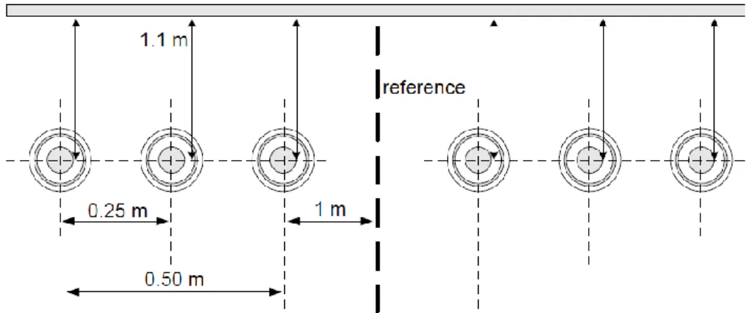
Figure 3-3 : RTWB ac 3-phase cable layout. ... 48
Figure 3-5 : RTWB ac 3-phase cable. Voltage waveforms at the sending end of the cores, comparison with the CP model. ... 49
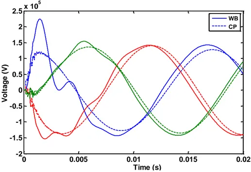
Figure 3-6 : RTWB ac 3-phase cable. Voltage waveforms at the receiving end of the cores, comparison with the CP model. ... 49
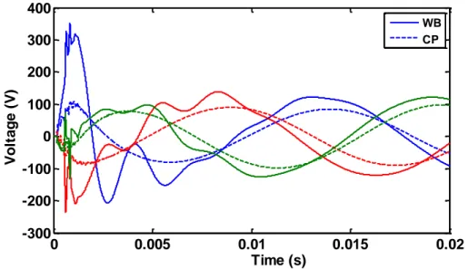
Figure 3-7 : RTWB ac 3-phase cable. Voltage waveforms at the sending end of the sheaths, comparison with the CP model. Insert; close up of the y and x axis. ... 50
Figure 3-8 : RTWB ac 3-phase cable. Voltage waveforms at the receiving end of the sheaths, comparison with the CP model. ... 50
Figure 3-9 : CP 3-phase aerial line circuit layout. ... 51
Figure 3-10 : CP 3-phase aerial line test circuit. ... 52
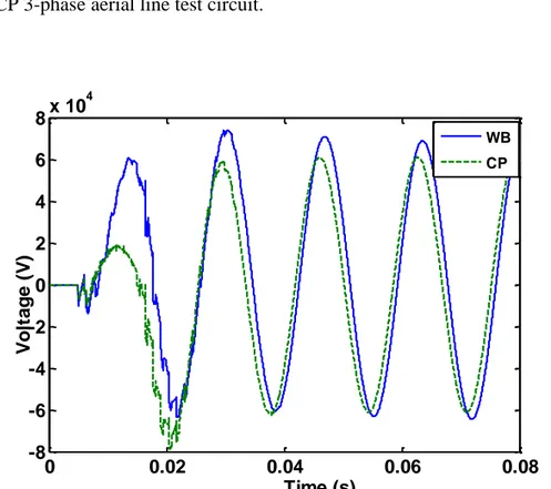
Figure 3-11 : CP 3-phase aerial line voltage waveform at phase b. ... 52
Figure 3-13 : RTWB 6-phase underground cable test circuit. ... 54
Figure 3-14 : RTWB 6-phase underground cable voltage waveform at receiving end of phase 1.54 Figure 3-15 : Transmission line configuration. ... 55
Figure 3-16 : Transmission network layout and data. ... 56
Figure 3-17 : Transmission network voltage waveform at phase b. ... 57
Figure 3-18 : Transmission network voltage waveform at phase b, close up. ... 57
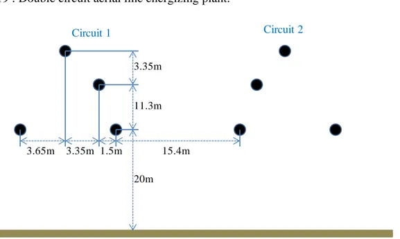
Figure 3-19 : Double circuit aerial line energizing plant. ... 58
Figure 3-20 : Double circuit aerial line layout. ... 58
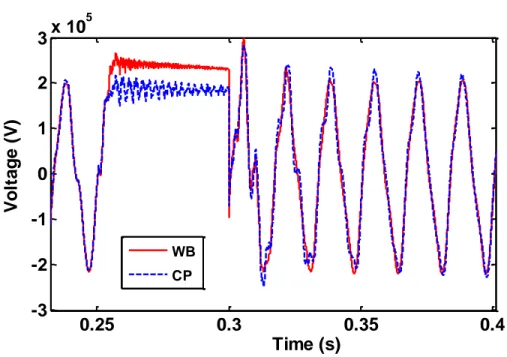
Figure 3-21 : Double circuit aerial line voltage waveforms at the consumption plant side of circuit 1, subplots correspond to phase a, b, c, close up on phase a, b and c, respectively. WB solid line, FD dashed line. ... 60
Figure 3-22 : Double circuit aerial line current waveforms at the consumption plant side of circuit 1, subplots correspond to phase a, b, c, close up on phase a, b and c, respectively. WB solid line, FD dashed line. ... 61
Figure 3-23 : BC HYDRO 9-phase aerial line layout. ... 62
Figure 3-24 : BC HYDRO 9-phase aerial line test circuit, WB vs FD. ... 63
Figure 3-25 : BC HYDRO 9-phase aerial line voltage waveform at the receiving end of the 5th phase, WB vs FD. ... 63
Figure 4-1 : RTE dc-cable system’s layout. ... 74
Figure 4-2 : RTE dc-cable real part of Yc diagonal elements. Solid line for results with 10 SPD, dashed line for results with 20 SPD. ... 75
Figure 4-3 : RTE dc-cable real part of H diagonal elements. Solid line for results with 10 SPD, dashed line for results with 20 SPD. ... 75
Figure 4-4 : RTE dc-cable test circuit (numerical test only). ... 76
Figure 4-5 : RTE dc-cable current waveforms at the sending end. Solid line are results with 20 SPD, dashed line are results with 10 SPD. ... 76
Figure 4-6: RTE dc-cable passivity test results for 10 SPD case. ... 77
Figure 4-7: RTE dc-cable passivity test results for 10 SPD case close up. ... 77
Figure 4-8: RTE dc-cable passivity test results for 20 SPD case. ... 77
Figure 4-9: Mader ac-distribution 12-phase cable layout. ... 79
Figure 4-10: Mader ac-distribution 12-phase cable test circuit. ... 79
Figure 4-11: Mader ac-distribution 12-phase cable. Real part of element (1,2) in matrix Hfitted with 2 poles. Solid line is the original value, dashed line is the fitted one. ... 80
Figure 4-12: Mader ac-distribution 12-phase cable. Passivity test result for a 0.01 level of absolute approximation error. ... 81
Figure 4-13: Mader ac-distribution 12-phase. Passivity test results close-up for the 0.01 level of absolute fitting. ... 81
Figure 4-14: Mader ac-distribution 12-phase cable. Real part of element (1,2) of Hmatrix fitted with 4 poles. Solid line is for original function values, dashed line is for fitted values. ... 82
Figure 4-15: Mader ac-distribution 12-phase cable. Passivity test results close-up for the 0.001 level of absolute fitting. ... 82
Figure 4-16: Mader ac-distribution 12-phase cable. Sending end current waveforms. Solid line corresponds to the 0.01 error level approximation case, dashed line is for the 0.001 error-level case. ... 83
Figure 4-17: EDF ac-cable layout. ... 85
Figure 4-18: EDF ac-cable traditional grouping case passivity test results. ... 85
Figure 4-19: EDF ac-cable no grouping case passivity test results. ... 86
Figure 4-20: EDF ac-cable, modal propagation function magnitudes. ... 87
Figure 4-21: EDF ac-cable test circuit. ... 87
Figure 4-22: EDF ac-cable nonpassive case receiving end voltage waveforms. ... 88
Figure 4-23: EDF ac-cable passive case receiving end voltage waveforms. ... 88
Figure 4-25 : BC HYDRO 9-phase aerial line. Voltage waveforms at the receiving end of circuit
1 nonpassive case. ... 89
Figure 4-26: BC HYDRO 9-phase aerial line traditional grouping case passivity test results. ... 89
Figure 4-27: BC HYDRO 9-phase aerial line traditional grouping case, passivity test results close-up. ... 90
Figure 4-28: BC HYDRO 9-phase aerial line, proposed grouping case, passivity test results, close-up around the low-frequency range. ... 91
Figure 4-29: BC HYDRO 9-phase aerial line, proposed grouping case, passivity test results, close-up. ... 91
Figure 4-30 : BC HYDRO 9-phase aerial line. Voltage waveforms at the receiving end of circuit 1 passive case. ... 92
Figure 4-31: BC HYDRO 9-phase aerial line, modal propagation functions magnitudes. ... 92
Figure 5-1 : RTWB 3-phase aerial line configuration. ... 106
Figure 5-2 : RTWB 3-phase aerial line test circuit. ... 107
Figure 5-3 : RTWB 3-phase aerial line receiving end voltage waveforms. ... 107
Figure 5-4 : RTWB 3-phase aerial line receiving end voltage relative errors. ... 108
Figure 5-5 : RTWB 3-phase aerial line receiving end current waveforms. ... 108
Figure 5-6 : RTWB 3-phase aerial line receiving end current relative errors. ... 109
Figure 5-7 : RTWB 2-phase underground cable layout. ... 110
Figure 5-8 : RTWB 2-phase underground cable test circuit. ... 110
Figure 5-9 : RTWB 2-phase underground cable receiving-end voltage waveforms. ... 111
Figure 5-10 : RTWB 2-phase underground cable receiving-end voltage relative differences. .... 111
Figure 5-11 : RTWB 2-phase underground cable receiving-end current waveforms. ... 112
Figure 5-12 : RTWB 2-phase underground cable receiving-end current relative differences. .... 112
Figure 5-14: RTWB 3-phase cable-sheath receiving-end voltage waveforms... 114
Figure 5-15: RTWB 3-phase cable-core relative differences. ... 114
Figure 5-16: RTWB 3-phase cable-sheath relative differences. ... 114
Figure 6-1: Discrete time-domain Norton equivalent of a multiconductor line. ... 120
Figure 6-2 : Flow diagram for RTWB implementation and its interface with SSN. ... 122
Figure 6-3 : Integer multiple buffer scheme. ... 125
Figure 6-4 : Interpolation buffer scheme. ... 125
Figure 6-5 : RTWB ac 3-phase cable sending-end core-voltages, real-time test. Solid line for EMTP-RV results dashed line for RTWB results. ... 129
Figure 6-6 : RTWB ac 3-phase cable sending-end sheath-voltages, real-time test. Solid line for EMTP-RV results dashed line for RTWB results. ... 130
Figure 6-7 : RTWB ac 3-phase cable receiving-end core-voltages, real-time test. Solid line for EMTP-RV results dashed line for RTWB results. ... 130
Figure 6-8 : RTWB ac 3-phase cable receiving-end sheath-voltages, real-time test. Solid line for EMTP-RV results dashed line for RTWB results. ... 131
Figure 6-9 : RTWB ac 3-phase cable sending-end sheath-voltages, solid line simulation with a 1s time step, dashed line simulation with a 10 s time step. ... 132
Figure 6-10 : BC HYDRO 9-phase aerial line test circuit, real-time test. ... 133
Figure 6-11 : BC HYDRO 9-phase aerial line circuit 1 receiving-end voltage-waveforms, real-time test. Solid line for EMTP-RV results dashed line for RTWB results. ... 133
Figure 6-12 : BC HYDRO 9-phase circuit 2 receiving-end voltage-waveforms, real-time test. Solid line for EMTP-RV results dashed line for RTWB results. ... 134
Figure 6-13 : BC HYDRO 9-phase circuit 3 receiving-end voltage-waveforms, real-time test. Solid line for EMTP-RV results dashed line for RTWB results. ... 134
Figure 6-14 : RTWB 6-phase cable voltage waveforms at the receiving end of phase a, real-time test. Solid line for EMTP-RV results dashed line for RTWB results. ... 136
Figure 6-15 : Transmission network voltage waveforms at Bus1, real-time test. Solid line for EMTP-RV results dashed line for RTWB results. ... 136
LIST OF ACRONYMS AND ABBREVIATIONS
BPA Bonneville Power AdministrationCP Constant Parameters
CTSS Continuous Time State Space DG Distributed Generation DTSS Discrete Time State Space EHV Extra-High Voltage
EMTP Electromagnetic Transients Program
EMTP-RV Electromagnetic Transients Program-Restructured Version EMTs Electromagnetic Transients
FACTS Flexible ac Transmission Systems
FD Frequency Domain
FDQ Frequency Domain Cable FFD Full-Frequency Dependent HIL Hardware in the Loop HVDC High-Voltage direct current RES Renewable Energy Sources RTWB Real-Time Wide Band
RTWB2B Real-Time Wide Band 2nd order Blocks TEM Transversal Electromagnetic
UHV Ultra-High Voltage ULM Universal Line Model
VF Vector fitting
LIST OF APPENDICES
CHAPTER 1
INTRODUCTION
1.1
Electromagnetic Transient Analysis for Modern Power Systems
Modern Power Systems are rapidly growing in complexity and size as they continue to incorporate new technologies. As a result, the time required for their study becomes excessive. For instance, HVDC interconnections, SVC, STATCOM, FACT devices, among others, each time are more popular. Distributed-generation (DG) devices and renewable energy sources (RES) are also current examples of new trends in power systems.
The aforementioned components and techniques usually are connected to the network using power electronic converters, giving as result a constantly changing network containing a broad range of frequencies. This situation can also be present in the case of power system faults. During normal operation, constant load and topology, electromechanical and electromagnetic energy exchanges are normally below the equipment rates. While, on the other hand, under switching events or system disturbances, the energy exchanges subject the circuit to higher stresses resulting from excessive current or voltage variations. These events often lead to equipment degradation or even total loss. The prediction of overcurrents and overvoltages is the main objective of Electromagnetic Transient Analysis.
Power system utilities and consultants rely each time more on digital simulators to test and to design electrical networks and apparatuses based on Transient Analysis results. For this reason, the use of real-time simulators is becoming more recurrent nowadays. Real-time simulators allow to test and verify equipment without using actual real networks because of their Hardware-in-the-Loop (HIL) capabilities. These analysis tools can perform simulations in a fraction of the time needed by their off-line counterparts.
Reliable and efficient power-network component-models are needed for real-time and parallel simulations. Power transmission power lines and cables are very important elements since they can represent up to 90% of the components in the Power System and provide natural time-decoupling between subsystems allowing parallel simulation. Transmission lines are often very difficult to simulate with the required accuracy. Inaccurate line/cable models may result into: 1) System overvoltage is underestimated, causing an underrating of the tested equipment which next can be the cause of a major blackout. 2) System overvoltage is overestimated, giving
as result an overrating of the equipment with the consequent overexpense. Thus, for economical and safety reasons is important to perform studies with the most accurate and efficient line/cable models.
This thesis focuses on line/cable models which are accurate, numerical efficient and suitable for real-time simulations.
1.2
State of the Art in Power Line and Cable Modeling
Presently, real–time and off-line simulators employ two types of line models: the Constant Parameters (CP) [1] and the Frequency Dependent (FD) [2] ones. The former is based on the assumption of line parameters being frequency independent and it is highly efficient, computationally speaking. It also is capable of simulating aerial lines and underground and submarine cables. Nevertheless, the assumption of constant parameters is correct only for steady-state analysis. At transient steady-state studies the CP model tends to overestimate voltage and current magnitudes, thus misrepresenting the transient phenomena mostly in underground cables where parameters are highly frequency dependent.
One of the most successful frequency-dependent line models perhaps was the FD-line one presented in [2]. The basic assumption in it is that modal transformations can be accurately attained through a real and constant matrix. The FD-line model is widely used because of its robustness. Its accuracy is also very good, except for cases involving underground and submarine cables, as well as highly asymmetric aerial lines. Recently, the FD line model has been reformulated to make it compatible with the Vector Fitting tool (VF) [3]. This results in a model with high numerical efficiency that is suitable for real-time simulations [4]. Since the late 1980s to present, a very active area of research has been the development of fully frequency dependent or wideband (WB) line models [3]-[7].
Nowadays, the most accepted WB model undoubtedly is the Universal Line Model (ULM) [5]. It is based on the traveling-wave principle and its parameters are obtained through the VF algorithm. ULM works well in most cases and, before the work being reported here, it was only available for off-line simulators. Nevertheless, the ULM still requires further development. In some situations one may not be able to achieve the desired accuracy with it or, if the fitting process delivers unstable poles, these have to be flipped to the stable region and this degrades its
accuracy. Moreover, there have been reports of cases where the fitting procedure fails to converge. Weighted Vector Fitting (WVF) [6] is a modification to VF that helps to overcome some of these problems and that can produce lower order realizations.
1.3
Problem Statement
For industrial-grade real-time simulators, the available line models are either of the constant parameters (CP) or of the frequency dependent (FD) class. CP line models are very efficient computationally speaking and are capable of simulating line and cables. However, this kind of model considers that line parameters are constant, i.e., they don’t vary with frequency. This assumption is correct only for steady-state analysis while, for transient analysis it is known that CP models tend to overestimate voltage and current magnitudes misrepresenting the transient phenomena mostly in underground cables where parameters are highly frequency dependent.
The FD line model is more accurate than the CP one since the former model takes into account the frequency dependence of line propagation functions. FD models work in the modal domain and perform the transformation between modal and phase domain by a single real constant transformation matrix. This feature makes the FD line model computationally efficient. Is also because of this feature that the model is inaccurate for simulating, highly-asymmetrical aerial-lines and underground and submarine cables.
Given the increasing use of underground/submarine cables for safety, environmental and economical reasons, the need for an accurate and reliable line/cable model, capable of performing simulations in real-time is evident. The lack of such model is thus the main motivation for the research reported in this thesis.
The Universal Line Model (ULM) or Wide Band (WB) line model is the most general, state-of-the-art line model presently available for off-line simulators. This model takes into account the full frequency dependence (FFD) of line parameters and works directly in the phase domain. This feature makes it highly accurate. At the same time also, its numerical efficiency is much lower than that of the CP line and FD line models.
Given the fact that the ULM is capable of accurately simulating aerial lines as well as insulated cables, its implementation in a time platform is highly attractive. However, real-time simulation imposes restrictions nonexistent in off-line simulations. In its current state the
ULM is not capable of completely meet those restrictions. It thus needs to be reformulated in order to meet the requirements imposed by real-time simulations. Furthermore, there are reports of cases where the ULM fails and results in unstable time-domain simulations [6] [7].
Thus, a major objective of this thesis is to overcome existing problems with the ULM. Other important objective is to achieve real-time performance while retaining accuracy and stability.
1.4
Thesis Objectives
General ObjectiveThe general objective of this thesis is to formulate and to implement a full-frequency-dependent (FFD) line/cable model for real-time and off-line simulators. This implementation should overcome most of the remaining limitations of the ULM. Major focus of this thesis is on the numerical efficiency, the accuracy and the stability of the implemented ULM or WB line model.
Specific Objectives
The obtained line/cable model must be solved much faster (at least two times) than existing full-frequency-dependent models. For this reason numerical efficiency must be dramatically increased.
The obtained line/cable model must be accurate and deliver comparable results to those obtained with already existing models. Nevertheless, in this thesis an acceptable compromise between speed and accuracy is searched.
The obtained line/cable model must be suitable for implementation in real-time platforms as well as in off-line simulators.
The obtained line/cable model must be stable and passive for all simulations. It must increase its level of generalization to solve existing problematic cases.
1.5 Contributions of this thesis
Because the main goal of this research is to develop and implement a full-frequency-dependent line model capable of simulating aerial lines as well as underground/submarine cables
for a real-time platform with the additional feature of being able to be implemented in offline platforms. The already existing WB model implemented in EMTP-RV is taken as the basis to develop more stable and faster line/cable models that not only improve upon the computational performance of its predecessor at offline simulations, but that also overcomes real-time restrictions while preserving accuracy. Passivity, stability and causality in the proposed models are also improved by identifying and curing several drawbacks within the fitting stage of the model.
The WB model basically consists in three main stages 1) line parameters calculation, 2) rational fitting or obtaining rational models and 3) time-domain iteration or solving line model equations in time domain. This research deals mainly with stage number three where the original WB model is modified to achieve a substantially increase in computational efficiency. In a lesser degree, this thesis deals with stage two where the fitting process is analyzed to obtain passive, stable and causal models.
At the original ULM, the VF tool or its modification WVF is used to obtain rational fits of the characteristic admittance and propagation functions matrices. One advantage of using this tool is that it delivers accurate and compact rational models. Nevertheless, an important disadvantage of this technique is that it may produce complex-conjugate pairs of poles thus forcing state variables and related equations to be declared as complex, even if obtained poles are real. This results in a loss of numerical efficiency, since the handling of real variables as complex increases the number of required sums at least by a factor of two and the number of real multiplications by a factor of four. In addition, all of the added sums and multiplications are trivial; that is, sums of zeros and multiplications by zeros. It is shown in Chapter 5 that for the case of complex conjugate state variables, the two states from a conjugate pair convey the same information and the computation of these two is redundant. This information leads to the development of a model here denominated “first order blocks” or “first order realizations” model. The proposed modification enables achieving a gain of up to 7 times in computational speed. This model is first implemented in Simulink and in EMTP-RV for offline simulations and, in the OPAL-RT real-time platform, for real-time simulations. The real-time version of the model is further named RTWB for real-time WB line model and is the first of its kind being implemented in a cluster-based real-time simulator.
It is also shown in Chapter 5 that complex-conjugate states are naturally eliminated by their combination into a single state ruled by a second order differential equation. The application of this idea results in a model that is called here as “second order blocks” or “second order realizations.” This modification permits achieving a gain of up to 8 times in computational speed with respect to standard implementations of the original ULM. The new model is further implemented in Simulink and in EMTP-RV for offline simulations. Even though, the second orders block model is not implemented yet in a real-time platform, this can be done with relative ease. This second model is here on called RTWB2B for real-time WB 2nd order blocks model.
RTWB and RTWB2B are not only several times faster than they predecessor they also provide accurate simulations. This is supported through several tests included in Chapter 5.
One problem encountered when using VF is that this tool does not guarantees passivity and therefore neither causality nor stability of the obtained rational models, thus leading to unstable or erroneous time-domain results.
At Chapter 4 several cases are analyzed and used to draw and overcome realized steps inside the fitting stage of the line model that if not well addressed may lead to nonpassive, unstable, or noncausal rational models. Such steps are 1) mode grouping, 2) representation of initial characteristic admittance and propagation factors matrices and 3) number of poles or fitting accuracy. The passivity test proposed in [8] is used to test for passivity inside the obtained rational models.
A general accepted practice on the modeling of multiconductor lines is that modes with nearly equal time delays and angles must be grouped in a single delay group for the sake of numerical efficency. It is shown at section 4.6.4 that the grouping of modes by taking into account angles and time delays only, can introduce stiffness into the fitting process ending up with a nonpassive, unstable and noncausal model. It is shown also in this section that by taking into account the mode magnitudes too, by means of a simple error comparison, the aforesaid problems are prevented.
It is also shown at Chapter 4 that by given a sufficiently large number of frequency points at the representation of the initial characteristic admittance and propagation matrices, nonpassivity problems can be avoided. The effect of the number of poles on passivity also is addressed at Chapter 4. It is reported there that the number of fitting poles is closely related to the
fitting error and that by increasing this number the fitting is improved and passivity violations are reduced to a small value as to obtain stable time-domain solutions.
The above mentioned three points are used as guidelines to avoid the lack of passivity in the obtained rational models, as well as to obtain accurate and stable time-domain simulations. These points are adopted with the models being proposed here. In consequence, these models are more stable than the original ULM. In sum the models proposed here not only are faster and accurate, but also are more stable than the original ULM.
CHAPTER 2
TRANSMISSION LINE ANALYSIS
Transmission line analysis has its basis on a pair of partial differential equations usually referred to as the Telegrapher’s Equations. For a lossless multiconductor line these equations are stated as follows: t x v L0 i (2.1) t x i C0 v (2.2)
where
v
and iare the respective vectors of conductor voltages and conductor currents, L0 is the matrix of self and mutual inductances of the line conductors and C0is the matrix of their self and mutual capacitances. Both, L0 and C0 are in per unit length units and are of order N×N for a line with N conductors.For the lossy-line case, the transmission line equations are stated more conveniently in the frequency domain: ZI V dx d (2.3) YV I dx d (2.4)
where V and I are the Fourier Transforms of
v
and i respectively, Z R jL is the matrix of self and mutual impedances of the line conductors, and, Y G jCis the matrix of their self and mutual admittances. Both matrices, Z andY , are in per-unit length units.The following equations often are used and correspond to an approximation of (2.3) and (2.4) obtained under the assumption of line-parameter matricesL,R,CandG being independent of the frequency
. Ri i L v t x (2.5)Gv v C i t x (2.6)
Nevertheless, the time domain equivalents of (2.3) and (2.4) should involve convolution operations. For instance, the following forms are due to Radulet, et.al. [9].
t t d t t x 0 ) ( ) ( r i i L v 0 (2.7)
t t d t t x 0v()g( ) v C i 0 (2.8)whereL0andC0 are as in (2.1) and (2.2), r(t)and g(t) are the respective matrices of transient resistances and transient conductances corresponding to the inverse Fourier transforms of
j R L L R 0 j G C C G 0
At most texts in the specialized literature, line equations usually are derived from well accepted circuit representations of transmission lines. Although this approach provides a rapid introduction to line analysis, it leaves out important aspects of the line transmission phenomena that are needed when developing a state of the art line model. Electromagnetic Theory, on the other hand, provides a complete description of line phenomena and this is the approach presented next.
2.1
Electromagnetic Basis of Line Theory
A transmission line essentially is a longitudinal array of parallel conductors. The purpose of this array is to guide electromagnetic (EM) waves along the line path. One basic assumption of Line Theory is that the transversal dimensions of a line (i.e., conductor cross-sections and distances) are smaller than one fourth the shortest wavelength involved in the wave propagation phenomenon. For a lossless line, this assumption implies that the only spatial mode supported by
the line is the transversal electromagnetic (TEM) one; that is, the mode in which the electric and magnetic fields are transversal to the line path.
For the case of lossy lines including imperfect conductors, a longitudinal component of the electric field appears and is associated to charge movement. A non-transversal component of the magnetic field can as well be produced by asymmetric distributions of currents inside the line conductors. In spite of the presence of those non-transversal EM-field components, transmission line analysis is extended to lossy lines under the assumption of these components being of much smaller magnitudes than those of their transversal counterparts. It is thus said that wave propagation is in quasi-transversal electromagnetic (or quasi-TEM) mode.
2.1.1 Single-phase case: first line equation
A one-conductor, or single-phase, transmission line actually consists of two parallel conductors being electrically insulated from each other. One of these conductors is taken as the reference one assigning to it a 0 V potential value all along the line. From here on, the reference conductor is labeled as the conductor 0. Figure 2-1 depicts a segment of a single-phase transmission line made of two cylindrical conductors. The actual transversal shape of the conductors is irrelevant for the analysis that follows. Included is in Figure 2-1 the oriented trajectory or pathABCDA which defines the rectangular surfaceS of width
z. Faraday’s Law being applied to the line segment states that the variations in the magnetic flux flowing through S will induce an electromotive force along the path ABCDA, that the magnitude of this force is proportional to the flux variation and that the force polarity is opposed to the flux changes. From the frequency-domain form of Faraday’s Law:
ABCDA s d j dl B s E (2.9)The closed-path integral at the left hand side (LHS) of (2.9) is decomposed next as the sum of the four line integrals along segments AB, BC, CD and DA:
DA CD BC ABCDA AB d d d d dl E l E l E l E l E (2.10)Figure 2-1 : Single-phase line segment. a) Lossless line
In the case of an ideal line, the line integrals along segmentsABandCDare zero, since there cannot be an electric field tangential to the surface of an ideal conductor. The line integral along segmentBCcorresponds to the voltage rise at point B with respect to pointC. Let this voltage be denoted asV(zz). The line integral along segment DA represents the voltage drop at point
A
with respect to point D which is denoted asV(z). Hence:
ABCDA z V z z V dl ( ) ( ) E (2.11)Consider now the right hand side (RHS) of (2.9) and assume that the width of rectangular surface S is sufficiently small as to permit neglecting of B-field variations along
z; hence:
A D y y s Bdy z j d j B s (2.12)B-field intensity is proportional to the currentI flowing through conductor 1 and returning through conductor 0. The following relation can thus be established:
x A B D C z y
I L Bdy A D y y 0
(2.13)The proportionality constant L0 in (2.13) is identified as the ideal line inductance in per unit of length. The subscript “0” is to indicate that this inductance accounts for magnetic fields outside the conductors, as (2.11), (2.12) and (2.13) are replaced in (2.9) the following relation is obtained: I L j z z V z z V 0 ) ( ) (
(2.14)On taking the limitz0, and on applying the inverse Fourier transform:
t i L z v 0 (2.15)
Expression (2.15) is the single-phase version of (2.1). a) Lossy line
For the case of a non-ideal line with imperfect conductors, the line integrals along segments AB and CD at (2.10) cease to be zero. Nevertheless,
z is taken sufficiently small as to permit neglecting E-field variations along it. Expression (2.11) is thus modified as follows:z E z E z V z z V d ABCDA ) ( ) 1 0 (
E l (2.16)where E1 and E0 are the respective longitudinal E-field components at segments AB and CD on the surfaces of conductors 1 and 0. From Ohm’s Law:
1 1 1 J E 0 0 0 J E
with1and 0 being conductor 1 and conductor 0 resistivities, and J1 and J0 are the respective current densities at segments
AB
and CD. Clearly both, E1 and J1 must be proportional to bulkcurrentIflowing through conductor 1. By the same token, E0andJ0must be proportional to bulk current Iflowing through conductor 0. The following relation can thus be established:
I Z E
E1 0 c (2.17)
with the proportional constant being
. ) ( 0 0 1 1 I J I J Zc
SinceJ1andJ generally are not in phase with 0 I, Zcis complex:
.
c c R j L Z c
Z represents an impedance due to the magnetic flux penetration inside imperfect conductors 1 and 0. Its real part R corresponds to the resistance of the two conductors in per unit of length. Lc is the internal inductance of the two conductors, also in per unit of length.
Let now expressions (2.12), (2.13), (2.15), and (2.16) be introduced in (2.9) and, after a rearrangement of terms: ZI z z V z z V ) ( ) ( (2.18) with ). (L0 Lc j R L j R Z
As the limit z0 is applied in (2.18), the following expression is obtained:
.
ZI dz dV
(2.19)
Note that (2.19) is the single-phase version of (2.3). Note also that the line inductance parameter L is the sum of Lc due to magnetic flux penetration inside the imperfect conductors and L0 due to magnetic flux outside at the insulation. The former term is strongly dependent on the frequency. As this dependence is neglected, the inverse Fourier transform of (2.19) yields:
t i L Ri z v
2.1.2 Single-phase case: second line equation
Figure 2-2 depicts a line segment as the one in Figure 2-1. This time, however, the rectangular surfaceS, of width
z and delimited by closed pathABCDA
, is wrapped around conductor 1. Consider further that trajectoriesAB and CD overlap. Figure 2-3 shows the surface S and its contourABCDA being extended. Ampere’s Law being applied to this contour states that the circulation of the H -field aroundABCDA is equal to the current passing throughS. This is stated mathematically as follows in the frequency domain:
S ABCDA d j d H l
E s (2.20)where
is the conductivity of the insulating material between the line conductors and
is its electric permittivity. The LHS integral of (2.20) is now decomposed in four terms:
DA CD BC AB ABCDA d H d H d H d H d H l l l l l (2.21)Since trajectoriesAB and CD are made to coincide in Figure 2-2 and one runs opposite to the other, the first and the third terms at the RHS of (2.21) cancel each other. Note in addition that points
B
and C coincide, same asD
and A. It is for this reason that the second and the fourth terms on the RHS of (2.21) are closed integrals. As Ampere’s Law is applied to the second term, the result isI(zz).The application of this law to the fourth term yieldsI(z). In sum:) ( ) (z I z z I d H ABCDA
l (2.22)Let the RHS of (2.20) be considered now. Figure 2-4 illustrates a closed surface S formed by surface S from Figure 2-2 and Figure 2-3 being wrapped around conductor 1, and by the two flat and lateral covers S1 and S2. If conductor 1 is perfect, the E-field passing through S1and
2
S is zero and the integral on the RHS of (2.20) can be replaced by the closed integral throughS :
S S d ds E s E (2.23)Figure 2-2 : Ampere’s law on conductor 1.
Figure 2-3 : Trajectory ABCDA and surface S unfolded.
x z y A B C D z E+jE
Figure 2-4 : Gaussian surfaceSSS1S2.
When conductor 1 is imperfect, but still a good conductor, the E-field at S1andS2 is negligible as compared to that at S and expression (2.23) is accurate. On applying Gauss’ Law in (2.23) enc S Q d
E sWith Qencbeing the total electric charge insideS. It is possible to think of Qenc as a linear charge densityq distributed alongl
z. By being
zshort enough, q can be considered constant land l S zq d
E s (2.24) lq is further related to V, the voltage of conductor 1 with respect to conductor 0, as follows
CV
ql (2.25)
where C is the line capacitance in per unit length. a) Lossless line x z y 2 S 1 S S 2 1 S S S S
Let be assumed in (2.20) that the line insulation is perfect (i.e.,
=0). The introduction of (2.22), (2.24) and (2.25) into (2.20) yields:CV j z z z I
( ) (2.26)Further application of the limit z0 and of the inverse Fourier transform in (2.26) results in the second Telegrapher equation:
t v C z i (2.27) b) Lossy line
Consider now that the line insulation presents a certain amount of conductivity (>0). As (2.22), (2.24) and (2.25) are replaced in (2.20) one obtains:
V C j G z z z I ) ( ) ( (2.28) where G
is the conductance in per unit length. On taking the limit z0
YV dz dI
(2.29)
withY G jCbeing the line admittance in per unit length. On neglecting the frequency dependence of G and C expression (2.29) can be approximated as follows:
t v C Gv z i
2.1.3 Multiconductor case: first line equation
Figure 2-5 depicts a short segment of a multiconductor line formed by N conductors plus the reference one labeled as 0. Note in the figure the oriented trajectoryABCDA defining the
rectangular area Si of width
z. Segment AB runs along the surface of the ith conductor, with Ni1,2,..., . Segment CD runs along conductor 0. As Kirchhoff’s currents law is applied in Figure 2-5, it follows that:
N k k I I 1 0 (2.30)Let the frequency-domain form of Faraday’s law be applied to trajectoryABCDA in Figure 2-5: i ABCDA j d
E l (2.31)with i being the total magnetic flux through surfaceSiproduced by currents Io,I1,...,IN. This total flux can be considered as composed byNpartial fluxes:
Figure 2-5 : Multiconductor line segment. Application of Faraday’s law.
x A B D C z y 0 I 1 I i I N I
N k k i i 1 ,
wherei,k is the kth partial flux produced by current Ik on conductor k, along with its return current Ik on conductor 0. Moreover, as each partial flux k is proportional to its associated currentIk :
N k k i z L ikI 1 0, (2.32)where the kth proportionality constant L0i,kis referred to as the mutual inductance (in per unit of length) between conductors i and k, or as the self inductance of conductor i when i=k. Note in (2.32) that the assumption has been made as toz being sufficiently small for neglecting variations of Ik and i,k along the z–axis.
a) Lossless line
Consider the line integral on the LHS of (2.31) and its expansion as in (2.10):
DA CD BC ABCDA AB d d d d dl E l E l E l E l E (2.33)Since conductors 0 and i are ideal, the integrals along AB and CD are zero, and the other two integrals amount to the voltage difference between points B and A on conductor i , both being referred to conductor 0:
ABCDA i i z z V z V dl ( ) ( ) E (2.34)As (2.33) and (2.34) are introduced in (2.32), and the limit z0 is taken, the following expression is obtained: N i I L j dz dV N k k i k i ; 1,2,..., 1 0,
or, in matrix-vector form:I
L
V
0
j
dz
d
(2.35)whereL0 is the matrix of line inductances (in p.u.l. units)
N N N N L L L L , 0 1 , 0 , 1 0 1 , 1 0 0 L
and V and I are the respective vectors of voltages and of currents at the N line conductors
. , 1 1 N N I I V V I V
Finally, application of the inverse Fourier transform in (2.35) yields (2.1); that is, the first of the Telegrapher Equations for multiconductor lines:
t
z
v
L
0i
b) Lossy lineConsider again the line integral on the LHS of (2.31) and its expansion. The values for line integrals along segmentsBCand DA have been previously established as V(zz) and V(z), respectively. As conductors 0 and 1 are not considered ideal any longer, the E-fields along
segmentsAB andCDare different from zero; still though,
z
is taken sufficiently small to neglect their variations with respect toz ; hence:z E z E z V z z V d AB CD ABCDA i i
E l ( ) ( ) (2.36)Since EAB is the value of the E-field along conductor i, this value must be proportional to currentIi: N i I Z EAB cnd i i i, ; 1,2,..., (2.37)
The term ECD, on the other hand, corresponds to the E-field alongECDconductor 0 being taken as reference. According to (2.30), currentI0is the sum of return currents
N I I
I
1, 2,..., . The value of ECD is thus composed by Nterms, each one being proportional to a return current: N i I Z I Z I Z
ECD ref ref ref N
N i i
i,1 1 ,2 2... , ; 1,2,...,
(2.38)
The application of (2.36), (2.37), (2.38) and (2.33) in (2.32), along with the limitz0, results in: N i I L j I Z I Z dz dV N k k k i N k k ref i cnd i k i i i ; 1,2,..., 1 , 0 1 , ,
(2.39)Expression (2.39) is further stated in matrix-vector form as follows:
ZI
V
dz
d
(2.40) with ref cnd GZ
Z
Z
Z
and , 0 L ZG j cnd N cnd cnd cnd cnd diag Z Z Z R j L Z ( ,1, ,2,..., , ) . , 1 , , 1 1 , 1 N refN refN N ref ref ref Z Z Z Z Z GZ often is called the matrix of geometric impedances as its elements depend, apart from the insulation permittivity, on the transversal line geometry [10].
2.1.4 Multiconductor case: second line equation
Consider the multiconductor line segment depicted in Figure 2-6 where the surface S defined by the closed trajectory ABCDA is wrapped around conductor i. In much the same way as in the single-phase case of subsection 2.1.2, Ampere’s law is applied toABCDA:
S ABCDA d j dl E s H (2.41)As in the single-phase case, the LHS of this expression amounts to the following currents difference: ) ( ) (z I z z I d i i ABCDA
H l (2.42)Figure 2-6 : Multiconductor line segment. Application of Ampere’s law.
Under the assumption of a perfect or a good conductivity for conductor i: x z y 0 0 V 1 V i V N V
encl S Q d
E s (2.43)The total charge being enclosed by the S-defined cylinder Qencl can be considered composed by N partial charges:
N i
encl q q q q
Q 1 2... ...
with each componentqkhaving its reciprocal qk at the kth conductor. Notice here that the reciprocal for qi is at conductor 0 (the reference one). Each component qk is, in addition, proportional toVi Vk, the voltage difference between conductors i and k, and the proportionality factor
zc
i,k is the capacitance between the two conductor segments i and k of length
z
. Hence:
N i k k k i k i i i i encl zc V z c V V Q 1 , , ( ) where
c
i,i
c
i,0. This last expression is further arranged as follows:
N k k k i encl z C V Q 1 , (2.44) with
c i k k i c C N m im k i k i 1 , , ,The introduction of (2.42), (2.43) and (2.44) into (2.41) yields
N i V C j z z z I z I N k k k i i i ,..., 2 , 1 ) ( ) ( 1 ,
![Figure 2-8 : Circuit representation of multiconductor traveling-wave line model. V0+-YcI0 + -ILVLYcH[I+Y V ]L C LH[I+Y V ]0C 0](https://thumb-eu.123doks.com/thumbv2/123doknet/2345384.34761/51.918.214.741.781.960/figure-circuit-representation-multiconductor-traveling-wave-model-ilvlych.webp)