Polar, Cluster and SuperDARN evidence for high-latitude merging during southward IMF: temporal/spatial evolution

HAL Id: hal-00329292

https://hal.archives-ouvertes.fr/hal-00329292

Submitted on 1 Jan 2003

HAL is a multi-disciplinary open access

archive for the deposit and dissemination of

sci-entific research documents, whether they are

pub-lished or not. The documents may come from

teaching and research institutions in France or

abroad, or from public or private research centers.

L’archive ouverte pluridisciplinaire HAL, est

destinée au dépôt et à la diffusion de documents

scientifiques de niveau recherche, publiés ou non,

émanant des établissements d’enseignement et de

recherche français ou étrangers, des laboratoires

publics ou privés.

Polar, Cluster and SuperDARN evidence for

high-latitude merging during southward IMF:

temporal/spatial evolution

N. C. Maynard, D. M. Ober, W. J. Burke, J. D. Scudder, M. Lester, M.

Dunlop, J. A. Wild, A. Grocott, C. J. Farrugia, E. J. Lund, et al.

To cite this version:

N. C. Maynard, D. M. Ober, W. J. Burke, J. D. Scudder, M. Lester, et al.. Polar, Cluster and

SuperDARN evidence for high-latitude merging during southward IMF: temporal/spatial evolution.

Annales Geophysicae, European Geosciences Union, 2003, 21 (12), pp.2233-2258. �hal-00329292�

Annales

Geophysicae

Polar, Cluster and SuperDARN evidence for high-latitude merging

during southward IMF: temporal/spatial evolution

N. C. Maynard1, D. M. Ober1, W. J. Burke2, J. D. Scudder3, M. Lester4, M. Dunlop5, J. A. Wild4, A. Grocott4, C. J. Farrugia6, E. J. Lund6, C. T. Russell7, D. R. Weimer1, K. D. Siebert1, A. Balogh8, M. Andre9, and H. R`eme10

1_{Mission Research Corporation, Nashua, New Hampshire, USA}

2_{Air Force Research Laboratory, Hanscom Air Force Base, Massachusetts, USA} 3_{Department of Physics and Astronomy, University of Iowa, Iowa City, Iowa, USA} 4_{University of Leicester, Leicester, UK}

5_{Rutherford-Appleton Laboratory, Didcot, UK}

6_{EOS, University of New Hampshire, Durham, New Hampshire, USA} 7_{IGPP, UCLA, Los Angeles, California, USA}

8_{Imperial College, London, UK} 9_{Uppsala University, Upsalla, Sweden} 10_{CESR, Toulouse, France}

Received: 10 January 2003 – Revised: 22 April 2003 – Accepted: 28 April 2003

Abstract. Magnetic merging on the dayside magnetopause often occurs at high latitudes. Polar measured fluxes of ac-celerated ions and wave Poynting vectors while skimming the subsolar magnetopause. The measurements indicate that their source was located to the north of the spacecraft, well removed from expected component merging sites. This rep-resents the first use of wave Poynting flux as a merging dis-criminator at the magnetopause. We argue that wave Poynt-ing vectors, like accelerated particle fluxes and the Wal´en tests, are necessary, but not sufficient, conditions for iden-tifying merging events. The Polar data are complemented with nearly simultaneous measurements from Cluster in the northern cusp, with correlated observations from the Super-DARN radar, to show that the locations and rates of merging vary. Magnetohydrodynamic (MHD) simulations are used to place the measurements into a global context. The MHD simulations confirm the existence of a high-latitude merging site and suggest that Polar and SuperDARN observed effects are attributable to both exhaust regions of a temporally vary-ing X-line. A survey of 13 mergvary-ing events places the location at high latitudes whenever the interplanetary magnetic field (IMF) clock angle is less than ∼150◦. While inferred high-latitude merging sites favor the antiparallel merging hypoth-esis, our data alone cannot exclude the possible existence of a guide field. Merging can even move away from equatorial latitudes when the IMF has a strong southward component. MHD simulations suggest that this happens when the dipole tilt angle increases or when IMF BXincreases the effective

dipole tilt.

Key words. Magnetospheric physics (magnetopause, cusp and boundary layers; magnetospheric configuration and dy-namics; solar wind-magnetosphere interactions)

Correspondence to: N. C. Maynard

([email protected])

1 Introduction

It is generally accepted that merging between the interplan-etary magnetic field (IMF) and the Earth’s magnetic field (Dungey, 1961) is the principal coupling mechanism for solar wind plasma entry to the magnetosphere. The nature, loca-tion, and temporal dependence of merging remain open ques-tions. The purpose of this paper is to provide evidence that merging often proceeds away from the equator.

Accelerated flows of magnetosheath plasma observed near the subsolar magnetopause (near the Earth-Sun line) provide in situ evidence of the merging process (Paschmann et al., 1979; Sonnerup et al., 1981). Minimum variance analyses of magnetic field measurements were employed to show that the magnetopause acted as a rotational discontinuity with a finite Bnormal, proportional to the merging rate. However,

establishing an unambiguous finite Bnormal can be difficult.

Jump conditions across the discontinuity satisfy the Wal´en relationship, indicating that the change in the ion velocity is proportional to the change in the magnetic field. Obser-vations of accelerated flows, often identified by “D-shaped” distributions in velocity space (Cowley, 1982), have been re-garded as standard signatures of merging (e.g. Gosling et al., 1982; Paschmann et al., 1986; Sonnerup et al., 1990).

X-type merging configurations with oppositely directed field lines (Levy et al., 1964) were generalized by Sonnerup (1974) to include merging between the antiparallel compo-nents of B, along a line that hinges about the subsolar point (Gonzales and Mozer, 1974). Crooker (1979) offered an al-ternate hypothesis in which merging occurs wherever magne-tospheric and magnetosheath field lines are aligned antipar-allel to each other. For most IMF orientations the antiparantipar-allel location is at high latitudes on the magnetopause. By high (low) latitudes, we mean in the general vicinity of the cusp (equator). Both hypotheses locate merging at the poleward

2234 N. C. Maynard et al.: High-latitude merging boundary of the dayside cusp during periods of purely

north-ward IMF. Merging has been definitively identified there by Scudder et al. (2002a).

One difficulty in locating the merging line relates to a lack of accelerated particles observed during magnetopause crossings. In fact, decelerated flows are encountered in the boundary layer (Eastman et al., 1976). Aggson et al. (1983) transformed electric fields measured by ISEE-1 at the magne-topause into a de Hoffman-Teller (H-T) reference frame (de Hoffman and Teller, 1950). Data measured by Polar were subjected to a Galilean transformation to a reference frame moving with a velocity VH T. In this reference frame the

electric field component perpendicular to the magnetic field transforms to zero. H-T reference frames exist for rotational but not for most tangential discontinuities. The transforma-tion will not remove the electric field internal in the layer in a tangential discontinuity (e.g. Lee and Kan, 1979). Thus, the identification of a H-T frame for ordering satellite mea-surements that holds internally in the current layer implies the traversal of a rotational discontinuity. In the H-T frame the plasma velocity is directed along the magnetic field and is equal to the local Alfv´en speed.

While increased velocities were observed during some ISEE-1 magnetopause crossings, Aggson et al. (1984) also reported decelerated flows. Moreover, they emanated from a merging site poleward of the satellite. Scudder (1984) calcu-lated that, as the merging site moved off the equator, the ex-haust velocity from the X-line should equal the sum from the merging acceleration and the local magnetosheath velocity at the merging site. Hence, the outflow velocity in inertial space may be significantly less than the Alfv´en speed. In a recent analysis of 69 magnetopause crossings, Phan et al. (1996) found that, of the 42 that “satisfied” the Wal´en test, 21 had velocity changes that produced normalized slopes on the av-erage of 0.6, which is less than unity predicted from a single component merging X-line. They concluded that (1) merg-ing sometimes occurs at latitudes higher than the satellite and (2) earlier studies that restricted merging sites to only equa-torial latitudes were biased to include only those events with significant acceleration (e.g. Scurry et al., 1994). Scudder et al. (1999) showed that the Wal`en test was better performed with electrons whenever currents were present. Under these conditions, the normalized slopes for the ion Wal´en test de-tected during the same crossings were often significantly less than 1, which does not match expectations. They showed that during many of these non-conforming crossings, the normal-ized slopes of the electrons were consistently near +/ − 1, as needed for a conclusive rotational discontinuity test.

In a recent study Maynard et al. (2001b) correlated rocket measurements of electric fields near the Northern-Hemisphere cusp with geoeffective interplanetary electric fields (IEF) measured upstream in the solar wind by the Wind satellite. They found that observed lag times were signifi-cantly less than those predicted for simple advection. The IMF was dominated by BXand the clock angle in the Y − Z

plane was near 90◦. The short lag time and the dominant BX

forced consideration of tilted phase planes of the IEF and

placed the location of merging at high latitudes in the South-ern Hemisphere. Whether merging followed the antiparallel hypothesis of Crooker (1979) or whether a small guide field was present could not be ascertained with the available data. Either way, a portion of the cusp in the Northern Hemisphere was responding to a merging source in the Southern Hemi-sphere. Within the same all-sky picture of the dayside cusp taken at Ny- ˚Alesund, responses to high-latitude merging in the Northern Hemisphere were also identified. Because of IMF BY, the cusp was bifurcated into source regions

origi-nating from high-latitude merging in the Northern and South-ern Hemispheres, while IMF BXcontrolled the timing of the

interactions in each hemisphere. Merging rates responded to small-scale variations of the IEF, as evidenced by elec-tric fields observed at the rocket and by 557.7 nm emissions captured in the all-sky images. Because of the strong BX,

the lag time was 14 min longer for the Northern Hemisphere merging site compared to the Southern Hemisphere site. The bifurcation of the cusp with BY and the need for

antiparal-lel reconnection under those conditions was also deduced by Coleman et al. (2001).

Weimer et al. (2002) utilized data from four satellites in the solar wind to show that lag times varied continuously and to construct the phase plane in an over-determined way. They demonstrated that the orientations of IEF phase planes change significantly on time scales of tens of minutes, and that the small-scale variations often remained coherent while propagating over 200 REin the solar wind. Both factors were

used by Maynard et al. (2001b) to reach the interpretation described above. Variable lag times from the shifting ori-entation of the phase plane of the IEF must be considered in any assessment of IMF influences on merging processes. Lag times do not, in general, remain constant.

Projections of the dayside cusp onto the ionosphere may be quite wide (Maynard et al., 1997). Plate 1 of Maynard et al. (2001b) indicates that signatures of high-latitude merg-ing in the local hemisphere may be significantly displaced from noon when IMF BY is large. Azimuthal plasma

ve-locity enhancements may be expected from the merging and subsequent J × B acceleration.

Cowley (1982) documented the ion signatures expected in the vicinity of rotational discontinuities that attend X-type merging lines. Near the outer separatrix, transmitted or celerated magnetospheric ions may be found, along with ac-celerated and incident magnetosheath ions. Near the inner separatrix, the incident or cold distribution is of magneto-spheric origin, while accelerated distributions from magne-tosheath sources may also be observed. Distribution-function isocontours in v||–v⊥phase space exhibit “D” shapes when

acceleration has occurred. Finding a “D” shaped isocon-tour displaced from the origin has been cited by Fuselier et al. (1991) as “strong evidence” that reconnection has oc-curred. Bauer et al. (2001) reported many magnetopause crossings that “satisfied” Wal´en tests using ion velocities but lacked clear “D”-shaped distributions. They attributed the missing “D” to pattern blurring by mirroring particles. By itself, a “D” shaped distribution is a necessary but not a

sufficient signature of merging, since ambipolar parallel elec-tric fields associated with electron pressure gradients can ac-celerate ions without merging (Scudder et al., 2002b).

A second signature of merging may be identified from wave Poynting fluxes (1E×1B)/µ0, where 1E and 1B are

the fluctuations as described below. When merging occurs, Alfv´en waves are launched to communicate information to magnetically connected regions (Atkinson, 1992). The as-sociated wave Poynting vector is directed away from the source since it represents escaping electromagnetic energy. This electromagnetic energy flux should be strongest along the separatrices. Again, this is a necessary but not sufficient condition for identifying merging events, since other mecha-nisms can generate Alfv´en waves that carry parallel Poynting flux.

Geotail was the first satellite to skim along the magne-topause, while moving parallel to the equatorial plane. Dur-ing multiple crossDur-ings, Nakamura et al. (1998) observed increased speeds accompanied by ion heating and inferred them to have come from distant merging sites. More recently, Kim et al. (2002) observed accelerated flows at the magne-topause near the subsolar equator. They interpreted changes in direction as evidence for component merging, with the separator moving north and south relative to the spacecraft. Phan et al. (2000) used Geotail and Equator S measurements on the dawn flank of the magnetopause to provide nearly si-multaneous observations of bi-directional flows from an X-line between the spacecraft in the equatorial region. This was for a nearly pure BZsouth condition.

In the 2000–2002 period, the 9 RE apogee for the Polar

satellite orbit has been close to the equator. On many days it spent long periods skimming along the magnetopause from south to north, roughly at quadrature to the Geotail orbital plane. Often the satellite either traversed the magnetopause very slowly, or failed to cross it completely. Thus, temporal variations may be clearly identified, but spatial scales are not as easily determined. If current layers are crossed slowly and merging occurs at high latitudes, one should not assume that observations of an inner separatrix near the equatorial plane will be followed by an observation of an outer separatrix. With the merging line located far from the spacecraft it is probable that only one separatrix will be observed. Merging may vary both temporally and spatially, occurring simulta-neously at multiple sites. High-latitude merging is expected to be more temporally variable, since an X-line will not be intrinsically stable when the tangential magnetosheath flow is super-Alfv´enic (Cowley and Owen, 1989; Rodger et al., 2001).

Evidence that merging proceeds away from the equator plane at high latitudes is seen in a number of the Polar skim-ming passes. In the following sections, we present time-varying observations from Polar, Cluster and SuperDARN acquired on 12 March 2002, to establish the temporal and spatial variability of the merging process. Using other events and comparisons to simulation results, we extend these ob-servations to show that high-latitude merging is more

com-mon than generally thought when the clock angle is less than 150◦_{and may occur at even greater clock angles.}

2 Measurements

Several Polar instruments contribute to this study. The Hydra Duo Deca Ion Electron Spectrometer (DDIES) (Scudder et al., 1995) consists of six pairs of electrostatic analyzers look-ing in different directions to acquire high-resolution energy spectra and pitch-angle information. Full three-dimensional distributions of electrons between 1 eV and 10 keV and ion fluxes with an energy per charge ratio of 10 eV q−1 to 10 keV q−1_{were sampled every 13.8 s. The electric field}

in-strument (EFI) (Harvey et al., 1995) uses a biased double probe technique to measure vector electric fields from po-tential differences between 3 orthogonal pairs of spherical sensors. In this paper we present measurements from the long wire antennas in the satellite’s spin plane. The Mag-netic Field Experiment (MFE) (Russell et al., 1995) consists of two orthogonal tri-axial fluxgate magnetometers mounted on nonconducting booms. Electric and magnetic fields were sampled at a rate of 16 s−1. Most of the presented data were spin averaged using least-squares fitting to sine waves.

The Advanced Composition Explorer (ACE) spacecraft is located in a halo orbit around L1 in front of the Earth to

monitor interplanetary conditions. The solar wind velocity was measured by the Solar Wind Electron, Proton, and Al-pha Monitor (SWEPAM) (McComas et al., 1998). A tri-axial fluxgate magnetometer measured the vector interplanetary magnetic field (Smith et al., 1998). We also use data from the Magnetic Field Investigation (Lepping et al., 1995) and the Solar Wind Experiment (Ogilvie et al., 1995) on Wind for cross-checks. Wind was executing a distant prograde orbit; hence, it generally had large Y coordinates in this interval.

On one of the studied days the 4 Cluster spacecraft passed through the cusp while Polar was skimming the magne-topause. Magnetic field measurements were made on each of the Cluster spacecraft by tri-axial fluxgate magnetometers (Balogh et al., 2001).

In addition to the measurements of the vector magnetic field, the configuration of the 4 Cluster spacecraft allowed estimates of ∇ × B to determine local current flows. The nominal separation distances between the s pacecraft at this time was ∼ 600 km. The electric field and wave instru-ment (EFW) monitored both electric field components in the ecliptic plane using biased double probes (Gustafsson et al., 1997). The Cluster Ion Spectrometer (CIS) experiment pro-vided 3-D ion distributions with mass per unit charge com-position using the Comcom-position and Distribution Function (CODIF) analyzer (R`eme et al., 1997). Ion measurements are available only from spacecraft 1, 3, and 4.

In addition to the satellite measurements, the Super-DARN coherent backscatter radar network provided infor-mation about ion convection in the high-latitude ionosphere over a wide range of local times (Greenwald et al., 1995). Single-component drift measurements from each of the radar

2236 N. C. Maynard et al.: High-latitude merging

Polar

Polar

0

0

10

10

-10

X

X

Y

Z

0

0

10

10

-10

Cluster

Cluster

Z

0

0

4

-4

5

-5

Y

0

0

-5

5

4

Z

X

d

a

b

c

Figure 1

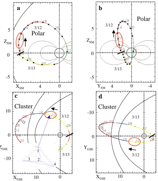
Fig. 1. Plots of the Polar orbit in the XZ and Y Z solar magnetospheric (SM)coordinate planes and of the Cluster orbit in the XZ and XY

geocentric solar ecliptic (GSE) planes for the 12 March 2001 event. The regions of interest are highlighted by the red ovals. The black line across the orbit track in each plot notes the start of the orbit trace. Nominal magnetopause and bow-shock configurations are indicted in panels a, c and d as appropriate. The circles at the origin represent the Earth. In panel c the insert shows the configuration of the 4 Cluster spacecraft, with Cluster 3 leading and Cluster 4 trailing. The tetrahedron configuration is maintained quite well during the interval of interest. Spacecraft separation is of the order of 600 km.

sites were iterated with an empirical model to estimate 2-dimensional vector drifts (Ruohoniemi and Baker, 1998).

3 Analysis methods

Our analysis concerns large-scale aspects of coupling be-tween the IMF and the magnetosphere-ionosphere system, from global- to meso-scale perspectives, where electron gy-rotropy applies and merging actually occurs (Scudder et al., 2002a). We do not consider the microphysics of the merg-ing process. Addressmerg-ing problems with simultaneous obser-vations from diverse locations properly constrains our inter-pretations. Analyzing Polar skimming passes presents chal-lenges and advantages. Since the magnetopause expands and contracts with changing solar wind conditions, multiple

crossings often occur. Polar sometimes remains in the vicin-ity of the magnetopause for hours. While this reduces our present knowledge about spatial structuring, it allows us to follow temporal responses to changes in the IMF and solar wind dynamic pressure, and thereby establish close correla-tions with external drivers. We correlate observed behaviors with temporal variations in other regions, such as in the iono-sphere as measured by SuperDARN, or in the outer cusp as measured by Cluster.

Interpretations of satellite measurements were tested for reasonableness through comparisons with predictions of sim-ulations using the Integrated Space Weather Model (ISM). ISM is a large-scale magneto-hydrodynamic (MHD) code developed by Mission Research Corporation to simulate the magnetosphere-ionosphere system from its front boundary

Merging location 1 1 1 1 Top view Dusk side view Front view 2 2 2 2 3 3 3 3 0 0 0 0 4 4 4 4 5 5 5 5

V_Y above the cusp initially positive Dawnward flow in cusp

J x B driven flow in cusp 2’ 3’ 4’, 5’ Merging location 0, 1 N H Potentials

a

b

c

d

e

f

Figure 2

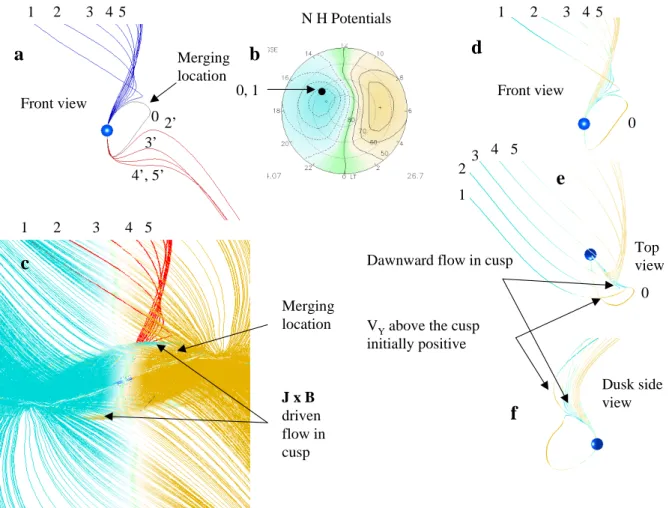
Fig. 2. Traced magnetic field lines from a MHD simulation using the Integrated Space Weather Model (ISM). Figure 2a shows a set of field

lines flowing away from a high-latitude merging site. Trace 0 is closed, and its origin in the Northern Hemisphere is shown in Fig. 2b to be between 15 and 16 MLT and 71◦latitude. All others are open. Figures 2d–f show three views of these same field lines colored with the Y component of the velocity. Figure 2c shows the complete set of first-open field lines traced from the ionosphere in each hemisphere and also colored with VY (see text).

40 RE upstream in the solar wind, to the base of the

iono-sphere near the Earth, and to deep in the magnetotail (White et al., 2001). Lacking the microphysics and resolution needed to accurately portray merging, ISM accomplishes the process through dissipation, either explicitly introduced by current dependent resistivity, or introduced by the code through the partial donor method (PDM) of Hain (1987), to maintain stability in the presence of steep gradients (see White et al., 2001, for more details). Through simulations of steady-state conditions or of responses to step-function driver variations, cause and effect relationships are easily iso-lated. This approach was used successfully by Maynard et al. (2001a; 2003a), to establish the sash (originally identi-fied in the simulations by White et al., 1998) as a reconnec-tion site, and to provide an explanareconnec-tion for short-lived, sun-aligned arcs emanating from the high-latitude open-closed boundary of the nightside auroral oval. Synergism between data analysis and the simulations provides a powerful tool for understanding the complex interactions of the solar wind with the magnetosphere-ionosphere system.

Polar often fails to traverse the magnetopause current layer

completely. Hence, we use two markers to identify occur-rences of merging. The first is to demonstrate the presence of accelerated parallel ion fluxes. Guidance comes from the interpretation of distribution functions given by Cowley (1982). Our second marker is the presence of parallel Poynt-ing flux. Active mergPoynt-ing must be communicated away from the site to other regions along the magnetic field lines by Alfv´en waves. Parallel Poynting flux, carried by waves prop-agating away from a source, can indicate where active merg-ing is proceedmerg-ing. Whereas the dc Poyntmerg-ing flux specifies the transport of energy by convective flow, the wave Poynt-ing flux, determined from 1E × 1B, measures energy flow carried by Alfv´en waves. To calculate the wave Poynting flux we subtract the average magnetic field (B0) and

elec-tric field (E0), determined using a sliding boxcar average of

3 min, from the measured field quantities. The above cross product is then taken. When the sharp changes in B occur as the magnetopause current layer is traversed, boxcar averages can allow variations from large-scale changes to contaminate the results. To avoid this problem we terminate the wave Poynting flux calculation at the edge of the current layer

2238 N. C. Maynard et al.: High-latitude merging

Figure 3

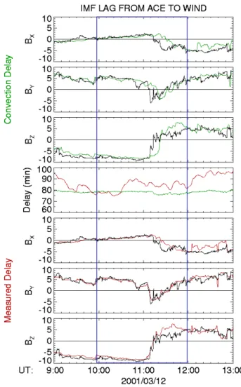
Fig. 3. Comparison of IMF data from ACE and Wind for 12 March

2001. (a)–(c) The comparison is made using the advection time (plotted in the green trace in panel (d). (e)–(g) The comparison is made using the variable lag time, calculated using the technique of Weimer et al. (2002) and shown by the red trace in panel (d). The region of particular interest is highlighted by the blue box. Note that the lag time is increasing prior to 10:40 UT, then levels off, and later decreases as the directional discontinuity is approached near 11:00 UT.

and resume the calculation when the major change in B has been completed. Calculations using spin-averaged data have a resolution of 6 s on Polar and 4 s on Cluster. Since there are other ways to generate Alfv´en waves, we look for the temporal concurrence of accelerated ions and parallel Poynt-ing flux, comPoynt-ing from the same direction, as the signatures of merging and indicators of its location with respect to the spacecraft.

To aid interpretation we establish the variable lag times for IMF features between ACE and Polar. The tilts of phase planes in the solar wind can change on short time scales (Maynard et al., 2001b; Weimer et al., 2002). The proper lags from ACE to Polar are adjusted by requiring that the IMF clock angle in the Y − Z plane be maintained across the bow-shock (Song et al., 1992). Whenever Polar is in the

Figure 4

Fig. 4. ACE magnetic field data between 10:00 and 13:00 UT in

minimum variance coordinates, where i is the direction of maxi-mum variance and k is the direction of minimaxi-mum variance.

magnetosheath, this technique can be used. When Polar is in the boundary layer or cusp, we must rely on the availability of at least two satellites in the solar wind, to apply the tech-nique described by Weimer et al. (2002) and to determine how lag times change.

Wherever possible we look for corroborating data from di-verse sites, such as SuperDARN or DMSP satellites in the ionosphere and/or Cluster in the cusp. An example in which data from all three sources can be utilized comes from the 11:00 to 13:00 UT interval on 12 March 2001.

4 Observations from 12 March 2001

4.1 Overview

On 12 March 2001, the Polar orbit skimmed the subsolar magnetopause while Cluster passed through the Northern Hemisphere cusp. Figures 1a and b show the X − Z and

Y − Z solar magnetospheric (SM) projections of the Polar orbit. Arrows indicate the direction of spacecraft motion. The region of interest lies inside the red ovals. Polar crossed it between 11:00 and 13:00 UT. At 12:00 UT the dipole was tilted tailward 0.3◦. Hence, the subsolar point is very close to the XSMaxis. Figures 1c and d present the X − Z and X − Y

projections of the Cluster orbits in GSE coordinates. Cluster crossed from the lobe to the magnetosheath above the cusp between 12:00 and 12:30 UT. Red ovals mark the period of interest. The insert in Fig. 1c depicts the tetrahedral config-uration of the Cluster satellites at 12:00 UT. Cluster 3 is in front, while Cluster 4 trails the other three. All spacecraft were located slightly post-noon. In addition, SuperDARN radar provided estimates of the ionospheric convection pat-terns. Thus, we can trace ionospheric responses to activity in the high-altitude cusp and on the dayside magnetopause, and from there to its sources in the solar wind.

Figure 2 provides a conceptual context for measurements acquired in the various regions. Traced field lines come from an ISM simulation using an IMF clock angle of 135◦, similar to the angle of 140◦for the 12 March magnetopause

cross-Magnetopause crossing Red

Figure 5

a

b

c

d

e

ACE data - Red: lag keyed to magnetopause; Blue: lag keyed to directional discontinuity

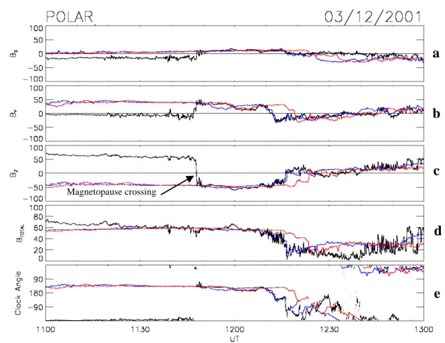
Fig. 5. Comparisons of the components, magnitude and clock angle of the magnetic fields measured at ACE (red and blue) and at Polar

(black). The lag time is set at 70.5 min for the red ACE traces, which is appropriate for the magnetopause crossing observed at 11:48 UT and the next 15 min. A lag time of 63.5 min (blue ACE traces) was used to bring into alignment the region around the directional discontinuities. The scale for ACE data is one-sixth of that marked.

ing. Last-closed field lines were found starting from the iono-sphere in each hemiiono-sphere. By moving poleward 10 km in the ionosphere from the trace point of each closed field line, we define a set of “first” open field lines. The last-closed and first-open field lines are labeled 0 and 1 in Fig. 2a. They map from the black dot in the potential pattern in Fig. 2b, near 15 MLT and 71◦magnetic latitude, and pass through the post-noon cusp. Field-line 0 also traverses the low-latitude region of the post-noon magnetopause. The closed field line maps to near the zero equipotential line between the two con-vection cells in the Southern Hemisphere.

To understand how the field lines change after merging, we have traced a number of field lines from a series of points along the Northern Hemisphere equipotential that passes through the origin of trace 0. The first 4 of these, labeled 2–5 in Fig. 2a, show how a field line evolves as it is dragged back over the magnetopause. A similar set of field lines was mapped from the equipotential contour in the Southern Hemisphere at the end of trace 0 and is labeled 2’–5’. Line 2’ probably pairs best with 2, although there is no way to trace the evolution of exact pairs from a merging site. A high-latitude merging site can be inferred to be located close to

where line 1 bends. Subsequent field lines show how they un-bend and traverse back through the cusp, as they are dragged antisunward by the solar wind.

Figure 2c shows the complete set of first-open field lines traced from each hemisphere. The field lines are colored ac-cording to VY. The Northern Hemisphere set of field lines

in Fig. 2a are colored red in Fig. 2c to show their position relative to the first-open field lines. The arrow points to the approximate locations of merging. Sharp bends in open field lines from the Northern Hemisphere indicate the general lo-cations where merging is occurring. Most pre-noon (post-noon) field lines have a negative (positive) VY. Exceptions

to this are in the cusp, where J × B forces from the currents associated with the curvature of newly-merged field lines to drive the flow westward (eastward) in the Northern (South-ern) Hemisphere (Siscoe et al., 2000). Note that the velocity separator is not the merging separator. The more vertical ve-locity separator results when the merging J × B forces over-come the normal hydrodynamic flow away from the nose. A faint line at about a 20◦tilt from the equator separates open field lines traced from the Northern Hemisphere from those traced from the Southern Hemisphere. The curvature of the

2240 N. C. Maynard et al.: High-latitude merging

Polar -- Hydra ions

Magnetosphere Boundary Layer Magnetopause Depletion layer Directional Discontinuity Northward IMF

e

a

b

c

d

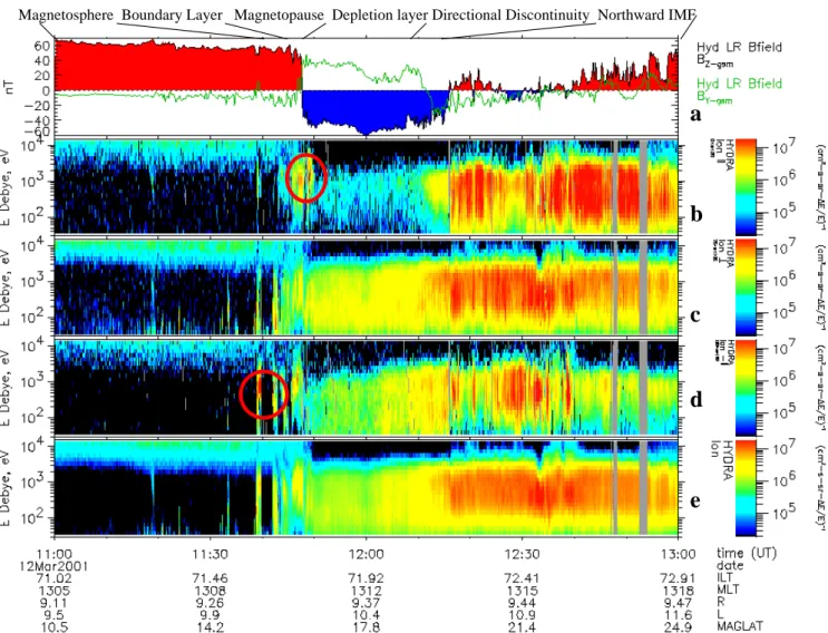
Fig. 6. Ion spectrograms and the magnetic field measured by Polar and plotted for the interval between 11:00 and 13:00 on 12 March 2001. (a) BZis shaded red (blue) for positive (negative) values. (b)–(e) Parallel, perpendicular, antiparallel and total ion energy spectra measured

by the Hydra instrument. The circles highlight parallel or antiparallel accelerated ion fluxes associated with a contact and a crossing of the magnetopause.

field lines in the upper left indicate that most are pulling away from high-latitude merging sites in the Southern Hemisphere. The fact that the velocity separator is so much different from the separation of traced field lines is further evidence that low-latitude component merging is not a dominant process in the simulation. Figures 2d–f display the front, top, and side views of the Northern Hemisphere’s closed and open field lines in Fig. 2a, colored with VY. Plasma flow in the

boundary layer on the closed field line (0) is toward dusk. Flow above (in) the cusp on line 1 is toward dusk (dawn). Subsequently, the flow is toward dawn, both above and in the cusp, as the field line is dragged back through the mantle.

The primary flow direction near the magnetopause and in the outer portion of the boundary layer is determined by the diversion of flow from pressure gradients away from the stag-nation region. Cowley and Owen (1989) have provided a

model of the flow, which combines the effects of the hydro-dynamic diversion of flow from a stagnation point with the magnetic tension effects from merging. Siscoe et al. (2002) argue that the stagnation point should, in fact, be a stagna-tion line along the magnetic field line that passes through the nominal stagnation point at the nose.

Thus, ISM suggests that with merging at high latitudes in the Northern Hemisphere, Polar should observe flow away from noon at its post-noon location. In the post-noon cusp, the open boundary layer can maintain movement toward dusk, corresponding to the flow in the magnetosheath. Due to merging, the outer separatrix should initially continue to move toward dusk (applicable to Cluster as it passes through the magnetopause above the cusp), while the inner separatrix (as well as the foot of the field line) is pulled toward dawn.

4.2 Interplanetary conditions

IMF measurements were made by the Wind and ACE space-craft located near (−37, −165, 8) and (227, −38, 4) RE,

re-spectively. Figures 3a–c show the three IMF components ob-served at the locations of the two spacecraft. Data are refer-enced to the UT of ACE measurements. Wind data (green) were lagged according to advection times based on the solar wind velocities measured at ACE (plotted as the green trace in Fig. 3d). The agreement between the traces in Figs. 3a–c is only moderate. This is especially evident beyond 10:00 UT. However, Weimer et al. (2002) showed that agreement could be improved by allowing for the lag time to vary on a minute-by-minute basis. Figures 3e–g show the same data (Wind data is colored red) using the calculated variable lag, which is plotted as the red trace in Fig. 3d. The variable lag reflects constantly changing tilts of IEF phase planes.

Our analysis focuses on the interval 10:00–12:00 UT. This interval is dominated by a large decrease in magnetic field strength between 11:12 to 11:50 UT (magnetic hole), shown in Fig. 4. A directional discontinuity occurs, probably ro-tational, during which GSM BY goes from positive to

neg-ative, and at 11:08 UT BZ becomes less negative,

preced-ing the sharp drop in B and reversal of BZ by a few

min-utes. The combined structure bears resemblance to a con-figuration observed in the interplanetary medium in front of a magnetic cloud on 24 December 1996, by Farrugia et al. (2001). The magnetic field decrease was interpreted as a slow shock, which, coupled with the preceding rotational discontinuity, could be the signature of an upstream recon-nection layer. The structure at ACE is approximately planar. Minimum variance analysis of the 3-h interval found a well-defined maximum variance plane with a normal component of −1.64±0.66, consistent with the reconnection interpreta-tion advanced by Farrugia et al. (2001) for the 24 December 1996 event. Figure 4 displays the three components and mag-nitude in principal axis coordinates. Polar observations at the magnetopause were acquired before and near the directional-discontinuity passage.

4.3 Polar observations

Polar encountered the magnetopause current layer several times before crossing the magnetopause at 11:48 UT. Vari-able lags help to establish the applicVari-able solar wind condi-tions at that time. Figure 5 compares the three components and magnitude of B, along with clock-angle measurements at ACE and Polar during the interval from 11:00 to 13:00 UT. Plot scales were adjusted to reflect the factor of 6 increase after traversing the bow-shock. The ACE data were lagged by 70.5 min (red traces). The lag was determined by best matching the Polar and ACE clock angles between 11:50 and 12:05 UT. Note that it is different from the lag between ACE and Wind, displayed in Fig. 3, because of the differ-ent locations. This lag is good through 12:08 UT, when the first of the two directional discontinuities seen in the ACE and Wind data were sampled by Polar in the magnetosheath.

Accelerated

magnetosheath Background_{magnetosphere}

a

b

c

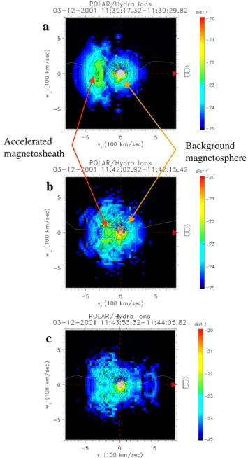
Fig. 7. Ion distribution plots for the interval of first contact with the

magnetopause indicated by the first circle in Fig. 5.

The lag time decreased as the directional discontinuity struc-tures approached. The variable lag time shown in Fig. 3d between ACE and Wind also was decreasing before the time of that structure, apparently due to the changed BX. In Fig. 5

the blue traces represent the ACE data with a 63.5-min de-lay, which is more appropriate for times at the arrival of the directional discontinuities. The decreased lag significantly improves the fit between 12:10 and 12:18 UT. The fit in the center of the magnetic hole has further variations in lag. The directional discontinuities have similar normals to those de-termined at ACE and at Wind, showing that they have main-tained coherence while passing through the bow-shock. Far-rugia et al. (1991) found that the planarity is maintained in the magnetosheath but the orientation may change somewhat

2242 N. C. Maynard et al.: High-latitude merging

Northward B; Southward Velocity

Southward B; Southward Velocity

Northward B; Northward Velocity

Southward B; Southward Velocity

Outside

Inside

Polar Magnetopause Crossing

Figure 8

a

b

c

d

Fig. 8. Ion distribution plots for the magnetopause crossing interval indicated by the second circle in Fig. 5.

on the passage through the bow-shock. Coherent passage through the magnetosheath is important for establishing the relative timing and interpretation of Cluster measurements. Note the presence of a magnetic hole centered at ∼12:30 UT, when the magnitude of B measured at Polar is less than the expected shocked and lagged magnitude from ACE. We note in Fig. 3 that B was also smaller at Wind in the middle of this structure, and suggest that ACE did not sample the mini-mum B within the magnetic hole. The clock angle at the time of the magnetopause crossing was approximately 140◦_,

sim-ilar to that of the ISM simulation discussed above relative to Fig. 2.

Figures 6b–e depict the energy spectra for the parallel, per-pendicular, antiparallel and total ion energy flux. To place these particle measurements in context, Fig. 6a shows Po-lar measurements of BZ (red for positive and blue for

neg-ative) and BY (green trace). The first contact with the

mag-netopause occurred at 11:39 UT, as indicated by a burst of

antiparallel ions (Fig. 6d). These fluxes occur while BY

re-versed to positive (Fig. 6a) and BZ(as well as the magnitude

of B) dipped. This is a good example of a partial entry into the magnetopause layer. Note too that bursts of parallel and antiparallel ion fluxes were seen during the magnetopause crossing at 11:48 UT. Both of these regions are highlighted by circles and are discussed in more detail below.

Two additional unique features of the spectrograms should be noted. First, there is a lack of plasma in the magne-tosheath just outside the magnetopause. In a separate pa-per, Maynard et al. (2003b) establish that this is a depletion layer. It is one of two types for southward IMF predicted by ISM simulations. Second, magnetosheath particles, includ-ing parallel and antiparallel fluxes, are also seen durinclud-ing the passage of the directional discontinuities. These fluxes are intense and have higher energies in the parallel components. Magnetosheath ions are often more biased toward perpen-dicular “pancake” distributions as the magnetopause is

ap-Red

Poynting Flux (black)

Magnetopause Directional Discontinuity

Figure 9

e

a

b

c

d

March 12, 2001

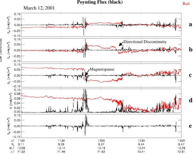
Fig. 9. Wave Poynting flux calculated from 1E × 1B and overlaid on the magnetometer traces (red), to provide context, for the 12 March

2001 interval.

proached. The dominance of the perpendicular fluxes is seen in low fluxes of the depletion layer region between 11:50 and 12:00 UT. The various regions are noted at the top of the plot. Figure 7 shows 3 ion-distribution plots accumulated be-tween 11:39 and 11:44 UT, within the first circle of Fig. 6d. The ion fluxes were shifted in velocity space by the perpen-dicular electron velocity, as the best proxy for the magnetic field line velocity. To create the distributions, symmetry was assumed around the parallel axis. Points of actual measure-ment are indicated by black dots (above parallel axis). No measurements exist between the white lines and the parallel axis, as this marks the closest approach of the particle detec-tors to the magnetic field direction in the analysis interval. For this time when Polar was on the magnetosphere side of the current layer, Fig. 7a shows a cold central core and an accelerated population, well displaced from zero, moving in the negative B direction, or coming from north of the space-craft. From expectations for locations on the inner separa-trix (Cowley, 1982), we interpret the accelerated population as being primarily of magnetosheath origin, but with a cen-tral core of reflected, accelerated, magnetosphere ions. Fig-ures 7b and c also show similar distributions but with smaller displacements. These distributions indicate a merging-line source to the north of Polar’s location.

Figure 8 displays 4 ion-distribution plots at the time of the 11:48 UT magnetopause crossing. Figures 8a and b were taken at locations on the inside of the current layer, while Figs. 8c and d are from locations on the outside of the cur-rent layer. Figures 8c and d indicate pancake-like magne-tosheath distributions, centered about the origin. An acceler-ated, cold magnetospheric population is seen along B, com-ing from poleward of the spacecraft. Observed perpendic-ular energies are comparable to the unaccelerated magneto-sphere distributions seen in Fig. 7. Figure 8a depicts an ac-celerated magnetosheath distribution with the cold magneto-spheric background. Again, the acceleration is from north of the spacecraft, which was located at ∼ 16◦magnetic latitude and 13:10 MLT. In Fig. 8b the distinctions are blurred; how-ever, we suggest that the ion acceleration was weaker and parallel to the magnetic field, or comes from a location equa-torward of the spacecraft. How far from the spacecraft is not discernable.

To strengthen our interpretation that these two magne-topause encounters reflect merging events located poleward of the spacecraft, the three components of the wave Poynting vector (S) are plotted in Fig. 9. The background magnetic-field components are provided as red lines for reference. Plots in Figs. 9a–d show the three GSM components and the

2244 N. C. Maynard et al.: High-latitude merging

Magnetosheath

Cusp

Mantle

Figure 10

Directional discontinuities

Current layer

a

b

c

d

Fig. 10. Cluster magnetic field measurements showing the components and magnitude during the passage of the satellites above the cusp.

Color codes for the traces are given at the top. Particular features discussed in the text are highlighted.

magnitude of the wave Poynting flux. Figure 9e shows the component of S parallel to B0. Between 11:39 and 11:44 UT SZ was negative (as was S||), in agreement with the

direc-tion of the ion acceleradirec-tion. In the traversal of the magne-topause current layer the calculation was interrupted to avoid contamination. The negative SZon the outside of the layer is

again in agreement with the direction of particle acceleration. Thus, these two encounters pass our empirical tests for merg-ing events at locations poleward of the spacecraft. In fact, we see enhancements in S at 11:39, 11:43, and 11:48 UT, sug-gesting intensification in the merging rate at those times.

The normal direction for the full magnetopause crossing was found using the minimum variance technique of Son-nerup and Ledley (1974). The normal component was small, but directed outward from the magnetopause, consistent with the merging occurring to the north of the spacecraft. As a further check on the rotational nature of this crossing, a suc-cessful Wal´en test across the full current layer using electrons (Scudder et al., 1999) resulted in a slope of nearly −1, indi-cating that the source of the rotation is above the spacecraft.

4.4 Cluster observations

Nearer to perigee, Cluster crossed spatial regions more quickly than Polar. Figure 10 presents the three GSM compo-nents, and the magnitude of the magnetic field measured by the 4 Cluster spacecraft between 12:00 and 12:30 UT. Cluster exited the mantle into the high-altitude cusp near 12:05 UT and crossed the magnetopause current layer out of the cusp into the magnetosheath between 12:13:50 and 12:15:00 UT. The magnitude of B increased as the satellites exited the high-altitude cusp. The biggest change during this crossing event was in the Y component. Each of the spacecraft saw the change at slightly different times, with Cluster 3 (Cluster 4) observing the change first (last), indicating that the change is primarily of a spatial nature. The order of crossing (3, 1, 2, 4) is consistent with the spacecraft configuration shown in Fig. 1c, showing Cluster 3 (4) leading (trailing). The subse-quent BYreversal between 12:16 and 12:17 UT did not result

from Cluster crossing back into the cusp. Rather, it reflects the encounters with the first of two IMF directional disconti-nuities observed earlier by Polar. Note that all four spacecraft

Polar Magnetopause Crossing

Cluster Magnetopause Crossing

Magnetic Hole IMF Reversal

IMF Reversal

Lag keyed to IMF reversal

Red

a

b

c

d

e

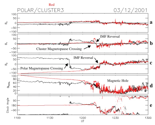
Fig. 11. Overlay of the Polar and Cluster 3 magnetometer data. The Cluster data is delayed −4 min. Note that once Cluster has exited the

current layer at the boundary the measured magnetic fields in the magnetosheath match in magnitude, direction and clock angle.

detected the negative shift in BY at nearly the same time,

in-dicating that this change is temporal. For a magnetosheath velocity of 100 km/s it would take 6 s for a feature to cross the satellite configuration. In fact, with a 4-min lag Clus-ter and Polar data are in excellent agreement afClus-ter 12:15 UT. Figure 11 compares Cluster 3 and Polar magnetic field data with this lag applied to the Cluster measurements. BZ

sub-sequently also reversed polarity as it did at the location of Polar. At that time the magnitude of B also decreased. Be-cause Polar saw the same directional and magnitude changes in the magnetosheath, we can safely conclude that these ex-hibit magnetosheath features rather than a reentry into the cusp. Key features of the combined data set are marked by arrows. As the constellation penetrated further into the mag-netosheath, the lag between Polar and Cluster observations decreased slightly. This fits expectations, since the obser-vations are made before the structure fully draped over the magnetopause. Minimum variance analysis of the magnetic field from each of the Cluster spacecraft at the magnetopause

crossing and the directional discontinuities provided normals that were stable between the spacecraft. They were also sta-ble between the magnetopause crossing and the BY reversal,

indicating that the discontinuity was draped along the mag-netopause orientation. All of the structure detected between 12:13 and 12:17 UT was planar on the scale of the spacecraft separation and aligned parallel to the magnetopause bound-ary. The normal to the BZreversal near 12:20 UT was

simi-lar, but slightly tilted.

Figure 12 presents spectrograms of ion energy fluxes measured in the antiparallel (140◦–180◦) and perpendicular (80◦–1◦) direction by CIS on Cluster 3, Cluster 1 and Clus-ter 4. In all cases the parallel flux (not shown) was much weaker. Three distinct features, which occur at staggered times, are highlighted by dashed lines. The first is an increase in energy seen at 12:06 UT by Cluster 3, 12:06:10 by Clus-ter 1 and 12:06:50 UT by ClusClus-ter 4. The increase is more pronounced in the antiparallel fluxes. The second feature is similar, occurring between 12:10:50 and 12:11:30. The

2246 N. C. Maynard et al.: High-latitude merging

Figure 12

Fig. 12. Ion energy spectrograms measured by the CIS instruments on Clusters 1,3 and 4. Antiparallel and perpendicular fluxes are shown

for each spacecraft. Cluster 3 is shown first as it is the lead spacecraft (see Fig. 1c).

third feature was seen in the perpendicular fluxes starting at 12:14 UT at Cluster 3. In this case the intensification starts at low-energies, then spreads to higher energies. From Fig. 10, we see that this increase started as each spacecraft exited the current layer. After this time ion fluxes are more typical of magnetosheath flowing away from the subsolar stagnation re-gion. Subsequently, measured energies were generally lower and the spectral width broader. Based on ion spectral charac-teristics, and the clear correlations of the magnetometer mea-surements with those from Polar, the features subsequent to 12:16 UT are of magnetosheath and solar wind origin. Be-tween 12:14 and 12:15 UT the antiparallel fluxes are intense

and higher in energy at Cluster 4, as expected from an active merging site located equatorward of the Cluster spacecraft.

Figures 13b–d show from Cluster 4 perpendicular H+

ve-locities (VH in blue) overlaid onto E × B velocities (VE in

magenta) in GSM coordinates for the interval between 12:00 and 12:20 UT from Cluster 4. The velocities compare very closely. A 1.5 mV/m sunward electric field offset has been subtracted from the GSE X-axis EFW electric field data to make this comparison. The magnitude of the offset was se-lected to maximize the correlation. Sunward directed er-ror fields are related to asymetries in the spacecraft sheath caused by photoemission (Cauffman and Maynard, 1974).

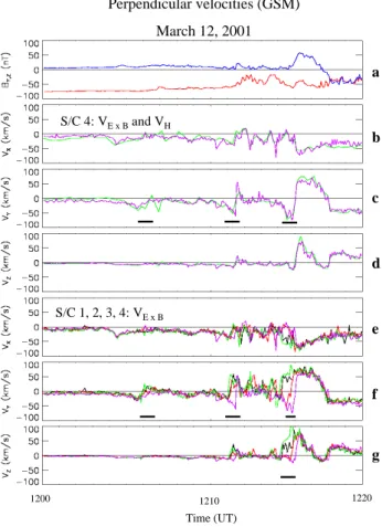
g a b c d e f Perpendicular velocities (GSM) March 12, 2001 S/C 4: V_{E x B} and V_H S/C 1, 2, 3, 4: VE x B Figure 13 1200 ₁₂₁₀ 1220 Time (UT)

Fig. 13. Velocity comparisons from Cluster. (a) The Y and Z

components of the magnetic field are shown for context. (b)–(d) The three perpendicular components of the ion velocity (blue) from Cluster 4 are compared with the velocity determined by E ×B. (e)–

(g) E × B velocities from all 4 spacecraft are overlaid (1 – black; 2

– red; 3 – green; 4 – magenta).

Figure 13a displays the Z (red) and Y (blue) magnetic field components for context. From Fig. 2 we expect that the ve-locity in the boundary layer was northward and toward dusk, except where active merging is occurring. Newly-merged field lines are pulled toward dawn soon after the merging takes place. Plasma velocities in the mantle have an anti-sunward component. Three regions of negative excursions in VH Y and VEY are seen and are marked by black

under-scores. Spacecraft 4 was the last of the Cluster spacecraft to traverse the boundary. VEfrom all four spacecraft are shown

in Figs. 13e–g. Similar offset corrections have been made on each of the other spacecraft. On Cluster 3 a negative excur-sion in VEY (green) was briefly seen just before 12:14 UT,

indicating that this apparent temporal enhancement in merg-ing lasted for over 1 min and had spatial scales on the or-der of the satellite separation. Other negative excursions in

VH Y occurred near 12:06 and 12:11 UT, in addition to the

larger one between 12:14 and 12:15 UT. Note also the signif-icant positive VZ, along with the enhanced VY that occurs as

the spacecraft exit the current layer into the magnetosheath. These velocities are consistent with the pictures in Fig. 2.

Figure 14

Poynting flux - Cluster - March 12, 2001

a b c d 1200 1210 1220 Time (UT)

Fig. 14. (a)–(c) The GSM components of the wave Poynting flux

overlaid from all four Cluster spacecraft for the interval between 12:00 and 12:20 UT. (d) The parallel Poynting flux overlaid for each of the spacecraft (1 – black; 2 – red; 3 – green; 4 – magenta).

Figures 14a–c present the GSM components of the wave Poynting flux in the same interval from the four Cluster spacecraft, calculated using the same method as with the Po-lar data. Figure 14d shows the parallel components. The wave Poynting flux is in the antiparallel direction, with peaks in the interval between 12:11 and 12:11:40, indicating that the satellite was above the source. Note the variability be-tween the 4 spacecraft, which indicates that the structure had dimensions of the order of the spacecraft separation. En-hancements are also seen after 12:13:50 UT, but the proxim-ity to the major current layer prevented the determination of the flux through the third region of velocity enhancement in Fig. 13. Small variations were also seen in the first inter-val of velocity enhancement. All three interinter-vals have been highlighted by the black bar for comparison to Fig. 13. The variability in both time and space suggests that the merging process is non-steady. Considering both the accelerated ions and the Poynting flux, we infer that Cluster is near the outer separatrix of an active merging site equatorward of the space-craft.

The Cluster configuration was favorable for determining the currents from curl B (Dunlop et al., 2002). Figure 15 displays local currents derived using a GSM coordinate sys-tem centered on Cluster 2. Also plotted are the divergence of B as a percentage of curl B and the magnitude of B at the locations of the four spacecraft. If the calculations were performed without error, Maxwell’s equations demand that

∇ ·B = 0. Currents determined where the divergence-to-curl ratio exceeds 50% should be treated with caution. In general, for this configuration, the expected error in J is at minimum 20%. Most of the large values of the divergence occur when the currents are small, highlighting their uncertainty. How-ever, when the currents are large, the divergence ratio is, in general, small, indicating where the calculated currents are

2248 N. C. Maynard et al.: High-latitude merging

Figure 15

a

c

b

d

e

Fig. 15. (a)–(c) Currents in GSM coordinates determined by the Curl B calculation. The calculation is centered on Cluster 2. (d) The ratio

of the divergence of B to the curl of B expressed in per cent. The ratio provides an indication of where the calculation is reliable (see text). The magnitude of B is given in the bottom panel for context.

reasonably valid. The curl B calculation integrates the cur-rents over the scale size of the tetrahedron (∼ 600 km). The largest current was detected between 12:14 and 12:15 UT and is primarily in the +Z and −X directions, noted by the green bars. It takes the four spacecraft over a minute to cross the main current layer, indicating its temporal stability. Thus, the center of this current should be well resolved. Coun-terclockwise Chapman-Ferraro currents on the dusk edge of the cusp have the anticipated direction. Note that between 12:16 and 12:17 UT, when the directional discontinuity was crossed, the current determination was less accurate; how-ever, the direction was −Z, opposite to the Chapman-Ferraro currents, confirming our interpretation that Cluster did not pass back through the boundary current layer.

JY is the most variable component showing both

polari-ties, although the strongest are currents in the −Y direction.

Some of the variability could occur if the current scale size was less than that of the Cluster configuration. Currents from structures of scale size less than 600 km may suffer from this error. Attention is directed to negative JY excursions

ob-served between 12:06 and 12:07, 12:11 and 12:11:40, and 12:14:30 and 12:15 UT, marked by red bars. There is also an associated smaller −JXexcursion. These correspond to

times when negative VH Yand VEY excursions were observed

by the Cluster spacecraft (black bars in Fig. 13). This sug-gests that these currents are related to temporally varying merging. Close to these times enhanced parallel ion and Poynting fluxes, our indicators of merging, were detected. The merging site must be south of the spacecraft, and the merging rate must be varying on minute scales to produce the observed three pulses. When we consider that Polar was showing temporally varying merging at high latitudes 20 min

previous, the implications are that this also involves time-varying high-latitude merging. The next section relates these enhancements to intensification of ionospheric plasma veloc-ities measured by SuperDARN radars.

4.5 SuperDARN measurements

Each SuperDARN radar measures the velocity component toward and away from the transmitter. To infer the large-scale flow pattern, the Ruohoniemi and Baker (1998) “map potential” technique was employed. Line-of-sight (l-o-s) ve-locity measurements from multiple radars are fitted to an ex-pansion of the electrostatic potential in spherical harmonics, to yield large-scale global convection maps. First, the l-o-s data are filtered and mapped to a polar grid. These “grid-ded” measurements are then used to determine a solution for the electrostatic potential distribution that is most consis-tent with the available measurements. Velocities should fall along plasma streamlines in the modeled pattern. Backscat-ter targets within the radar field-of-view are not always avail-able, and significant areas exist outside the reach of the radar system. The statistical model of Ruohoniemi and Green-wald (1996), parameterized by IMF conditions, is used to stabilize the solution in regions where no measurements are made. Figure 16 presents dayside Northern Hemisphere ionospheric convection patterns, each averaged over the in-terval given at the top. Dotted concentric semicircles indicate lines of constant magnetic latitude in 5◦_{increments. Noon is}

located at the top of each pattern. During the period from 11:00 to 12:15 UT, SuperDARN was observing velocity en-hancements in the 14 to 15 MLT region between 70 to 75◦. Figures 16a and b show these enhancements by comparing two consecutive patterns near the 11:48 UT Polar magne-topause crossing. The orange circle highlights the region of velocity enhancement, indicated by increased numbers of red drift vectors in the right pattern compared to the left. Note that the enhancement is localized, in the same region that the open-closed field line pair is mapped to in the simulation depicted in Fig. 2b, and occurs 1–2 min after the enhanced parallel fluxes were seen at Polar. We suggest that the delay is related to differences in Alfv´en travel times. The signature in the ionosphere should lag that in the outer cusp by the or-der of a minute, due to Alfv´en wave propagation time. The SuperDARN patterns show numerous increases in velocity in this general area over the hour-plus period.

To show the time variability, a search was made in the SuperDARN data for the largest velocity in the region and its location. The magnitude, the components, and the loca-tion are plotted in Fig. 17. The time of the three enhance-ments in merging observed at Polar are noted by the verti-cal red lines. The corresponding velocity peaks at Super-DARN are highlighted by the red dots. Within the interval that Polar was probing the magnetopause, these are the only peaks. Subsequent peaks starting at 12:06 UT correspond to the interval where Cluster observed evidence of merging. Figures 16c and d show SuperDARN potential patterns and vectors for intervals that contain the first 2 velocity and

cur-rent enhancements at Cluster, depicted in velocities in Fig. 13 and currents in Fig. 15. Returning to Fig. 17, the velocity and current enhancements observed by Cluster and noted by the blue dots correspond to three velocity enhancements seen at SuperDARN. Those periods are noted by the blue ovals in Fig. 15. Since Cluster observations come from above the cusp on the outer separatrix, while SuperDARN is looking at the response at the foot of the field line, we suggest that the difference in times from Alfv´en wave propagation may be less than those observed by Polar. Note that no peaks above 800 m s−1occur after 12:15 UT. The velocity enhancements are in the region predicted by the simulation as being tied to high-latitude merging. The correspondence with the Po-lar magnetopause merging encounters suggests that Super-DARN and Polar are observing the opposite exhaust regions of a time-varying active high-latitude merging line. Continu-ing the correlation with Cluster, we are able to relate 3 more peaks in the SuperDARN velocities to time varying merging. The implications from considering the 2-h period of Super-DARN velocities is that the rate of merging varies often and considerably. The location may be just as variable.

4.6 Summary of the 12 March observations

From the observations presented above we may conclude for this day when the IMF clock angle was about 140◦that:

1. Polar, while skimming the nose of the magnetosphere, observed the effects of merging at high latitudes. Ac-celerated ions and wave Poynting flux were used as dis-criminators for the existence of merging. While the ex-act location of merging is not discernable from the data, it was above the spacecraft, which, in turn, was well above the component merging line location of Gonza-lez and Mozer (1974).

2. The merging rate was temporally varying, as indicated by both Polar and Cluster measurements.

3. SuperDARN observed enhancements in the flow in the ionosphere associated with these time-dependent merg-ing events observed at Polar. Polar, near the subso-lar magnetopause and SuperDARN in the high-latitude ionosphere, monitored both exhaust regions. From Su-perDARN observations we may also infer that varia-tions in the merging rate occurred continuously for more than an hour.

4. Cluster continued the correlation, placing the merging location below the satellite, which was located above the cusp. Both SuperDARN and Cluster observed ef-fects of time-varying merging.

5. Flow in the boundary layer and adjacent magnetosheath was generally away from the sub-solar region unless specifically diverted by merging. In a time dependent process, boundary layer flows vary continuously. 6. Two directional discontinuities and an associated

2250 N. C. Maynard et al.: High-latitude merging

1148-1150 UT

1150-1152 UT

1206-1208 UT

1210-1212 UT

d

a

b

c

Figure 16

SuperDARN - March 12, 2001

Fig. 16. Potential patterns and drift vectors determined from SuperDARN measurements for 4 intervals related to merging observations at

Polar and Cluster. The regions of interest are highlighted by the orange circles.

from the solar wind. The effects of these were observed by both Polar and Cluster.

7. Adjacent to the magnetopause, Polar observed a deple-tion layer, implicadeple-tions of which are further discussed by Maynard et al. (2003b).

5 Other events

Table 1 summarizes all of the merging events investigated to date, using wave Poynting flux and accelerated ions as discriminators. The events are organized according to the applicable IMF clock angle (third column). The fourth col-umn lists our best estimates of the merging locations. Note that the measurements provide information about whether the site is to the north or south the spacecraft. For a number of events we calculated the difference between the spacecraft location and the component merging line of Gonzalez and Mozer (1974). The differences are listed in the last column. During periods when the ions and Poynting flux propagated from north of Polar and the differences are significant, we labeled the merging location as being at high latitudes. The last column also comments on special circumstances

prevail-ing durprevail-ing each pass. If the ions and Poyntprevail-ing flux originated south of Polar, we were unable to discern from the mea-surements alone, whether the merging line is near the equa-tor or at high southern latitudes. Question marks indicate instances when assigned merging locations are ambiguous. The event of 05:48 UT on 1 April 2001 is labeled “close” because Mozer et al. (2002) interpreted signatures obtained during this magnetopause crossing as indicating proximity to the separator. In some cases we relied on SuperDARN mea-surements and ISM predictions to identify merging locations. These are noted in column 5. The event at 05:05 UT on 16 April 2000 included episodic encounters with fluxes from the north and south of the spacecraft. We address this further in the discussion. During the two passes of 31 March 2001, Po-lar did not enter the dayside magnetosphere because of the high activity and very compressed conditions. In each case Polar crossed from the mantle to the magnetosheath above the cusp as noted in the comments.

For applicable clock angles of 150◦or less in the events of Table 1, merging generally occurred poleward of the space-craft and was inferred to be at high latitudes. This conclusion should be substantiated in the analysis of more events; how-ever, it is clear that one must consider high-latitude

merg-Cusp Mantle Cluster Polar

a

b

c

d

e

Fig. 17. The maximum velocities and

their locations determined by Super-DARN for the interval between 11:00 and 13:00 UT.

ing as an option when interpreting events driven by a signif-icant IMF BY. Our measurements suggest that low-latitude

or component merging is indicated only when BZ was the

dominant IMF component.

6 Discussion

We have used observations of accelerated particles and wave Poynting vectors as our primary indicators as to whether merging has occurred and, if so, where. As demonstrated above, both flux types provide necessary, but not sufficient, conditions for identifying merging events. Establishing that the boundary is a rotational discontinuity adds a third nec-essary indicator of merging. Since rotational discontinu-ities may be found in any magnetohydrodynamic flow, in-cluding those that do not involve reconnection, a success-ful Wal´en test, by itself, is not a sufficient test to conclude

that merging geometries have been encountered. However, the magnetopause-sheath interface is generally thought to in-clude such a structure to form a locally open boundary. In this spirit a successful Wal´en test (with electrons) with slope

±1 is associated with a potential merging site, whose X-line separator will, in general, be well removed from the space-craft’s trajectory. Successful Wal´en tests to establish the ro-tational discontinuities, in conjunction with observations of accelerated particles, have been the primary empirical cri-teria for identifying merging events. Recently, Scudder et al. (2002a) reported small-scale breaking of both ion and electron gyrotropy, as well as parallel electric fields within merging regions poleward of the cusp during an interval of northward IMF. In the events considered here, observations were made away from the separator region. Thus, we rely on signatures recognized as strong indicators, but not con-clusive proof, that merging has occurred. With this caveat in