HAL Id: pastel-00552045
https://pastel.archives-ouvertes.fr/pastel-00552045
Submitted on 5 Jan 2011HAL is a multi-disciplinary open access archive for the deposit and dissemination of sci-entific research documents, whether they are pub-lished or not. The documents may come from teaching and research institutions in France or abroad, or from public or private research centers.
L’archive ouverte pluridisciplinaire HAL, est destinée au dépôt et à la diffusion de documents scientifiques de niveau recherche, publiés ou non, émanant des établissements d’enseignement et de recherche français ou étrangers, des laboratoires publics ou privés.
To cite this version:
Victor Romero. Spiraling Cracks in Thin Sheets. Mechanics of materials [physics.class-ph]. Université Pierre et Marie Curie - Paris VI, 2010. English. �pastel-00552045�
de Santiago de Chili
THESE DE DOCTORAT DE L’UNIVERSITE PIERRE ET MARIE CURIE
Spécialité
Sciences Mécaniques, Acoustiques et Electroniques Présentée par
M. Victor ROMERO Pour obtenir le grade de
DOCTEUR de l’UNIVERSITÉ PIERRE ET MARIE CURIE
Sujet de la thèse :
SPIRALING CRACKS IN THIN SHEETS
Soutenue le 9 Décembre 2010 Devant le jury composé de :
M. BICO José Maître de Conférence M. CERDA Enrique Professor, Directeur de Thèse M. CLÉMENT Eric Professeur
M. GÉMINARD Jean-Christophe Directeur de Recherche M. HAMM Eugenio Assistant Professor
M. RICA Sergio Directeur de Recherche, Rapporteur M. VILLERMAUX Emmanuel Professeur, Rapporteur
M. ROMAN Benoit Chargé de Recherche, Directeur de Thèse
Université Pierre & Marie Curie - Paris 6 Bureau d’accueil, inscription des doctorants Esc G, 2ème étage
15 rue de l’école de médecine 75270-PARIS CEDEX 06
Tél. Secrétariat : 01 44 27 28 10 Fax : 01 44 27 23 95 Tél. pour les étudiants de A à EL : 01 44 27 28 07 Tél. pour les étudiants de EM à MON : 01 44 27 28 05 Tél. pour les étudiants de MOO à Z : 01 44 27 28 02 E-mail : [email protected]
Departamento de F´ısica
In Cotutelle with
Universit´e Pierre et Marie Curie
Spiraling Cracks in Thin Sheets
V´ıctor Manuel ROMERO GRAMEGNA
Advisor in Chile: Dr. Enrique CERDA VILLABLANCA
Advisor in France: Dr. Benoit ROMAN
Thesis submitted to the Faculty of Science of the University of Santiago and University Pierre et Marie Curie in partial fulfilment of the requirements for the
degree of Doctor of Philosophy.
Santiago, Chile December 9, 2010
V´ıctor Manuel ROMERO GRAMEGNA
Advisor professor in Chile:
Dr. CERDA Enrique
Advisor professor in France:
Dr. ROMAN Benoit
Committee:
Dr. BICO Jos´e
Dr. CL ´
EMENT Eric
Dr. G ´
EMINARD Jean-Christophe
Dr. HAMM Eugenio
Dr. VILLERMAUX Emmanuel
Dr. RICA Sergio
Thesis submitted for the degree of Doctor of Philosophy.
Santiago, Chile December 9, 2010
Opening a package made of a thin film is not always a satisfying experience. The crack is not easily controlled even though we try to guide it with our hands. This “freedom” for the crack propagation is connected with the many possibilities of thin sheets to deform. Indeed, deformation and fracture are highly related be-cause deformation is the source of the energy required to propagate a crack. In this way, finding and explaining regular crack paths in thin sheets improve our un-derstanding of the fracture of these objects. In previous scientific works, regular crack paths in brittle thin sheets have been reported. We can mention convergent tears obtained by peeling or tearing a flap of a thin sheet; also it is possible to find oscillatory cracks when a thin sheet is cut through by a moving blunt object. In this work we present two very robust, reproducible, divergent families of cracks paths in a brittle material (bi-oriented polypropylene, BOPP, usually used in pack-aging). These two final crack paths are characterized as similar logarithmic spirals although they are the outcomes of two very different set-ups. A first logarithmic spiral is the result of propagate only one crack by pushing an edge of a thin sheet, in this case the crack propagates because the material is been stretched and therefore the energy associated with the fracture propagation is “stretching en-ergy”. In the second spiral experiment, we propagate only one crack on the same material, but now we are tearing up in such a way that the energy, feeding the crack, comes from out of plane deformation. This last procedure not only results in a spiraling regular crack, but also in a beautiful and very complex out-of-plane structure of the tear.
Cette th `ese ´etudie la rupture de plaques ´elastiques fragiles dans deux configu-rations qui conduisent `a une propagation en spirale : soit `a la suite d’ ´etirement provoqu´e par le contact avec un indenteur qui pousse toujours sur la mˆeme l `evre de la fissure, soit en tirant une languette perpendiculairement au plan de la plaque. Dans le premier cas, on ´etudie exp´erimentalement la r´eponse ´elastique du syst`eme, et on pr ´edit les conditions pour la propagation, ainsi que la direction, `a partir du crit `ere du maximum du taux de restitution de l´energie. En suivant ces r´esultats, une propagation en spirale logarithmique est alors pr´edite, ce qui est confirm´e par les exp ´eriences.
Malgr ´e un chargement m´ecanique diff´erent, la deuxi`eme exp ´erience se ram`ene `a un probl`eme tr `es similaire, avec cependant un taux de croissance de la spirale logarithmique plus faible. Ce processus de rupture `a croissance exponentielle a fait lobjet dun d´ep ˆot de brevet pour l’ouverture facile d’emballage.
Dans les deux exp´eriences, on observe cependant que la forme des spirales est perturb´ee de fac¸on similaire par l’anisotropie des propri´et ´es du mat ´eriau. Une extension du mod`ele est propos´ee pour tenir compte de ces effets.
En este trabajo de tesis presentamos dos experimentos en que trayectorias de fracturas sumamente reproducibles son obtenidas en l´aminas delgadas fr´agiles. En ambos casos, a partir de configuraciones iniciales sumamente simples y peque˜nas, las trayectorias obtenidas son espirales logar´ıtmicas de gran tamao.
Nuestro primer experimento consiste en un crack que se inicia desde un corte recto hecho en una l´amina delgada y que es forzado a propagarse por medio de empujar con un objeto s´olido. Este procedimiento genera una espiral de gran tamao r´apidamente. Mostramos en este trabajo que la forma final no de-pende del movimiento del objeto con el que empujamos, siempre y cuando sea un solo borde de la l´amina el que se empuja. Bas´andose en teor´ıa cl´asica de fracturas hemos sido capaces de modelar y explicar esta trayectoria final de la fractura. Adem´as a trav ´es de una serie de experimentos hemos validado y probado nuestras suposiciones y predicciones. Finalmente, a partir de la carac-terizaci ´on geom´etrica de la espiral obtenida, mostramos evidencia del efecto de la anisotrop´ıa del material usado en el proceso de fractura.
El segundo experimento presentado en este trabajo se inicia con una configu-raci ´on inicial conveniente. Removiendo una pequea cantidad de material creamos un ”convex hull”, luego hacemos un pequeo corte y tiramos la ”lengeta” de ma-terial que se genera. Como resultado de este proceso solamente una fractura se propaga, dando lugar nuevamente a una trayectoria final en forma de espiral logar´ıtmica. En este caso la complejidad de la deformaci´on hace muy dif´ıcil mod-elar el fen´omeno, sin embargo, bas´andonos en simples argumentos geom´etricos hemos encontrado una relaci´on que conecta la fuerza requerida para forzar el crack y la energ´ıa que se requiere para romper la l´amina delgada.
el resultado final es similar. Este an´alisis nos entrega condiciones para que la fractura final sea divergente.
In this process many people and institutions have been very important. My first words of gratefulness are to my advisor professors, Enrique Cerda and Benoit Roman, for their guidance in the understanding of the physics, not only as a pro-fession but a way to observe every thing around us. Their advise and method-ology have been deeply inspiring. I can not forget to mention the great patience they have had with me, and my hope is that I did not dissapoint them. Thank very much to both of you.
Because of the way in which this work has been done, I have been very fortunate to met many people all around the world, who have help me in many different ways. I can not forget to mention John Bush, Pedro Reis and his lovely wife Ines, and Pascal Raux, who receive me in Boston, where I spend three months learning and working at the applied math group in MIT.
I have to thanks many people from the academics sphere, because in them I found many help in the develop of my work. Professors Eugenio Hamm, Fran-cisco Melo, Jos Bico, Juan Carlos Retamal, Dora Altbir, among many others, from which I learn not only formal academic contents, but also the big commitment with the develop in science.
In this process people who has always been next to me no matter what situation are my very good friend from both, Paris and Santiago. Juan Palma, Sebas-tian Michea, Juan Fuentealba, Fransico Santiabaez, Alejandro Pereira, Antonella Rescaglio, Daniela Briceo, Franco Tapia, David Mu˜noz, Gonzalo Quiroga and last but not less Miguel Pi˜neirua. I have counted with all this people to become the person I am, and I hope that I always will have them to my side.
expect to be for the rest of my life, I love you very much.
This work has not been possible without the financial support of Conicyt with their national PhD Grant, CNRS, Scat-alpha Project, Smat-C, and Anillo Project (Dy-namics, Singularities, and Geometry of matter out of Equilibrium).
Abstract i R ´esum ´e ii Resumen iii Acknowledgements v List of Figures xi 1 Introduction 1
1.1 Thin Sheets: Crumpling, Wrinkling, Folding and Creasing . . . 1
1.2 Fracture of Thin Sheets . . . 7
1.3 Convergent Versus Divergent (or Pulling versus Pushing) . . . 10
1.4 Spirals . . . 12
1.5 Thesis Outline . . . 13
2 Spiral Rupture With a Blunt Object 14 2.1 Spiral Experiment . . . 15
2.2 Tool path dependence . . . 18
2.3 Model . . . 21 vii
2.3.2 Fracture Propagation . . . 30
2.3.2.1 Geometrical Variation . . . 32
2.3.2.2 Griffith’s criterion and second Variation of the energy 34 2.3.2.3 Fracture Propagation Law. . . 35
2.3.2.4 Model Confirmation . . . 37
2.4 Three different stages in the Spiral . . . 40
2.5 Spiral Results . . . 47
2.5.1 Numerical Simulation of the Spiral Growth . . . 47
2.5.1.1 A Local Method to Find the Spiral Pole . . . 49
2.5.1.2 Global Method to Define a Pole of a Spiral . . . 50
2.5.1.3 Measuring β in the experiments . . . 51
2.5.2 Experiments . . . 51
2.6 Anisotropy. . . 57
2.6.1 Experiments with Highly Anisotropic Materials . . . 57
2.6.2 Anisotropic Model . . . 61
2.7 Conclusion . . . 67
3 Tearing Spiral 70 3.1 Experimental set-up . . . 71
3.2 Geometrical characterization of the Spiral . . . 74
3.3 Pulling forces . . . 81
3.4 Geometrical Characterization of the Initial Seed. . . 85
3.5 Easy Opening. . . 88
4 Conclusions 95
4.1 Spiraling Rupture With a Blunt Object . . . 95
4.2 Tearing Spiral . . . 97
4.3 General Conclusions . . . 98
Bibliography 99 A R ´esum ´e Franc¸ais 107 A.1 Introduction . . . 107
A.2 Chapitier 2 . . . 110
A.3 Chapitre 3 . . . 114
B Resumen Espa ˜nol 116 B.1 introducci´on . . . 116
B.2 Capitulo 2 . . . 119
B.3 Cap´ıtulo 3 . . . 123
C Basics Notions in Fracture and Elasticity Theories of Thin Sheets 125 C.1 Elasticity. . . 125
C.1.1 Elemental Relations in Elasticity . . . 125
C.1.2 Energy Storage in Thin Sheets . . . 127
C.2 Fracture Mechanics . . . 129
C.2.1 Fracture Modes. . . 129
C.2.2 Griffith Criteria . . . 131
C.2.3 Brittle, Quasi-static Crack Propagation, Stable . . . 131
1.1 Examples of crumpling, wrinkling, and creasing. . . 4
1.2 Illustration of converging tear experiment . . . 11
2.1 Pictures of the experiment “spiral rupture with a blunt object”. . . 15
2.2 Illustration of the possibles places where the blunt object can push the edge of the film . . . 16
2.3 Resulting experimental tear. . . 17
2.4 Tool tracking experiment . . . 18
2.5 Tool Trajectories and its respective resultant crack paths.. . . 19
2.6 Diagram of the configuration for energy storage in the system. . . . 21
2.7 Experimental diagram of the energy storage when a tool pushes a lip of a thin sheet.. . . 22
2.8 Data from experiments with different lengths and different thickness sheets. The penetration of the tool is given by the quantityd/L. . . . 23
2.9 Data from experiments with different lengthsL and sheets with dif-ferent thicknesses. The penetration angle of the tool is given by the quantityd/L. . . . 24
2.10 Exponent law for the energy storage process . . . 25
2.11 Non-symmetric experimental measure of force. . . . 29 xi
2.12 Force measurements in a non-symmetric experimental configuration. 29
2.13 Geometry of the system configuration. . . . 31
(a) Geometry before fracture. . . . 31
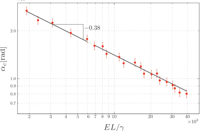
(b) Geometry after the crack, of lengths, propagates a distance δs. 31 2.14 Critical value of penetration angle αcas a function of the dimension-less quantity EL/γ plot with red dots. The black line corresponds to the linear fit of the logarithmic rectification of the collected data. . 38
2.15 Convex hull illustration.. . . 40
2.16 Initial stage for the spiral formation . . . 41
2.17 Second stage for the spiral formation . . . 42
2.18 Oscillatory crack path. . . 42
2.19 Final stage for the spiral formation . . . 43
2.20 Geometry in a logarithmic spiral. . . . 44
2.21 Numerical functionality betweencot φ and β. . . . 46
2.22 Illustration of the bases use to simulated the path formation. Top.-Example of the results of the simulation in the first stage of the spiral formation. Bottom Right.- Example of the results of the simulation in the second stage of the spiral formation. Bottom left.- Example of the results of the simulation in the final stage of the spiral formation. 48 2.23 Geometry in a logarithmic spiral. . . . 49
2.24 Diagram of the procedure to find the pole. . . . 51
2.25 Determination of the orientation of the Film. An illustration of the three experiments. . . . 52
2.26 Experimental measurements of the radius r, normalized with the initial sizero, from three experiments. Red and green circles are
ex-periments with a same initial orientation to the incision. Blue circles are data from an experiment initiated with a perpendicular orientation. 53
2.27 Crack propagation angle β as a function of the angle of the spiral, θ. inset The angle β as a function of the orientation in the film θg . . 55
2.28 Spiral made with a very anisotropic material. . . . 58
2.29 Illustration of the lines passing through the kinks intersecting in the pole. . . . 59
2.30 Radius (distance to the pole) as a function of angle, for two spirals initiated with perpendicular orientations in a very anisotropic material. 60
2.31 Case of a very anisotropic spiral. Crack propagation angle β as a function of the angle of the spiral, θ.inset The angle β as a function
of the global orientation in the film θg . . . 61
2.32 Illustration of the geometry used to compare the fracture energy and the direction of the crack. . . . 63
2.33 With red, blue and green circles, the values of β− "β#, are plotted. With black circles we present2(γ − "γ#)/γ. The inset presents the measures of γ(θ!
). . . . 65
3.1 Illustration of the initial cut. . . . 71
3.2 Illustration of the experimental set-up. . . . 72
3.3 Initial stages of the propagation. Note the 3D ”pine-tree” shape.. . . 74
3.4 Final tear from propagating a crack by pulling.. . . 75
3.5 Normalized distance from the pole O to all the points in two spirals initiated with perpendicular orientations. . . . 77
3.6 Measurements of β as a function of the spiral angle. Inset The
same data presented as a function of the absolute orientation in the film. . . . 78
3.7 Superimposed measurements of β collapsed in one period for both spiral experiments. With blue dots is plotted β from a pushing spiral, the dots in red are the measurements of β from a pulling spiral. . . . 79
3.8 Left.-The elastic pine-tree.Right.-The Internal structure of the
elas-tic pine-tree.. . . 81
3.9 Measurements of the pulling force versus time. The data for exper-iments with films of30µm (lower curve), 50µm (center curves) and 90µm (high curves) . . . 83
3.10 Initial Configuration. Geometrical frustration of the secondary crack. 85
3.11 Initial Configuration. Mechanical frustration of the secondary crack.. 86
3.12 Illustrations of an unsuccessful initial configuration: Left.- Initial
configuration made by removing a disk of material and a straight notch. Right.- Evolution of the morphology of the convex hull when
the crack advances. In this case the perimeter of the convex hull contains two discontinuities, hence two cracks nucleate at points T and B. . . . 88
3.13 Illustration of the optimal initial configuration for the spiral creation. . 89
3.14 Easy opening using our method to remove the packaging for a com-pact disk. . . . 91
3.15 The final shape of the crumpling structures in the elastic pine-tree. . 92
3.16 Sequence of pictures showing the formation of crumpled structures. 93
Introduction
1.1
Thin Sheets: Crumpling, Wrinkling, Folding and
Creasing
Thin sheets are defined as objects with one dimension (thickness,t) that is much
smaller than the other two. Thickness usually goes from some hundreds of mi-crons, as for example a sheet of paper, adhesive tape, normal packaging materi-als, etc., to a few nanometers, as in graphene sheets, lipids and nanoparticle films
and polymer coatings (these systems have a very small aspect rationt/a, where
a is the characteristic length for the width and length of the sheet). Mechanical
properties like bending and stretching stiffness (we useB for bending stiffness
andY for the two-dimensional stretching modulus) decrease with thickness,
mak-ing these objects flexible and soft; the ubiquitous examples of soft matter sys-tems. Behaviors typical of soft system, such as wrinkling, can be observed in a macroscopic flexible rubber sheet, but also in a semiconductor silicon crystal a few nanometers thick, usually associated as a stiff material due to its high Youngs
Modulus (102 GPa) [1].
The same thickness reduction explains why a smaller number of material con-stants are needed to describe a thin sheet (two for an elastic isotropic sheet, three
for an elastic isotropic body [2,3]). Similarly, when one dimension is reduced, a
strong coupling between geometry and mechanics is concomitant. Pure geomet-rical concepts, such as the Gaussian and mean curvature, or differential geometry theorems such as the Theorema Egregium play a significant role in describing a thin sheet [4,5]. Isometric deformations, preserving the first fundamental form, are observed in elastic sheets when confined. Lipids are assembled into membranes
of zero mean curvature to minimize surface area [6]. Thus, there are
geometri-cal constraints that need to be fulfilled independently of the specific nature of the sheet material.
In recent years, there has been growing interest to identify the specific modes of deformations in thin sheets satisfying these geometrical requirements. Phenom-ena like crumpling, wrinkling, creasing and folding are some examples of these possible modes of deformation that, although previously studied in works by Wag-ner, Reissner [7]. Mansfield [3], Sheppard [8], Biot [9], and others, have now been analyzed with new theoretical, numerical and experimental techniques. These research efforts are not only driven by a quest for knowledge. The interest in de-veloping technologies at smaller and smaller scales has posed new questions and challenges for engineers and scientists to understand and control the mechanical behavior of these objects.
Crumpling a paper sheet shows many of the geometrical and physical ideas that
are used in the analysis of thin sheets. In [10], Professor Thomas Witten has made
work to understand the localization of energy along ridges [11] provided a first glimpse of the complexity and richness of the phenomena involved in thin sheets. This complexity can be observed in a crumpled piece of paper: when it is un-folded it is possible to observe permanent deformations distributed randomly on it and a resulting structure characterized by sharp points connected by ridges. This permanent deformation indicates concentration of stresses in those points and ridges. The stress concentration distribution is not trivial nor intuitive, underlying a focusing mechanism of the energy that is intimately connected to geometry. Since resistance to membrane stretching is linearly proportional to membrane thickness
(t), and membrane bending goes with thickness cubed (t3), the ease of bending
versus stretching increases for thinner films [12]. As a result, thin films primarily
respond to loads by bending rather than stretching, and approximate geometri-cal solutions can be obtained by studying isometric deformations of the initial flat geometry. This purely geometrical view fails in regions of high curvature that are necessary to connect the four possible isometric deformations of a flat sheet: a plane, a cylinder, a cone and a tangent developable [4,5].
These isometric deformations and regions of high curvature have been studied
by several groups [13–16]. Ridges and point singularities show beautiful scaling
laws that are another characteristic feature in the study of thin sheets, for exam-ple, the mean curvature scales ast−1/3
in a ridge [11] and a point singularity [17]. These scaling laws have been checked by numerical simulations, indirect
experi-ments and theoretical arguexperi-ments [10]. There are no analytical solutions available
for these deformations due to the highly nonlinear nature of the equations describ-ing them.
These structures show some degree of randomness that have motivated theo-retical efforts to use probability distributions in the analysis of crumpling [18–20]. More modestly, but perhaps more applicable, other researchers have used the
same ideas of crumpling to evaluate the collapse of packaging structures [21].
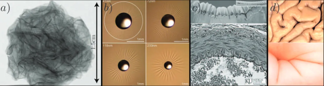
Figure 1.1: a.-Image extracted from a video made by D. Cambou and avaible in
the internet. It is a reconstruction of X-ray computerized tomography made of a1.5
cm crumpled aluminum foil. b.- Figure extracte from reference [22], in this figure
the number of wrikles depends of the thickness of the polystyrene thin sheet.
c.-Image extracted from reference [23], in the top image the controlled experiment is presented, the bottom image is a histological slide of a muscular artery cross-section, where it is possible to appreciate the resembles with biologycal systems.
d.- Image extracted from reference [24], in the top picture the sulci in a primate
brain is presented. In the bottom picture the arm of an infant. Representative sulcus structures.
The analysis of wrinkling patterns has been also an important area of research based on the possibility of using them in metrology. Beginning with the work of
Bowden et al. [25], who studied the wrinkling of a film on top of an elastic
sub-strate, we have seen the appearance of new techniques to measure the
these patterns is defined by the relation2πt(Ef/3Es)1/3 whereEs andEf are the
Young modulus of the substrate and film respectively. Thus, measuring the wave-length, thickness and Youngs modulus of the substrate gives Youngs modulus of the film. The same ideas have been used to take advantage of wrinkling patterns
generated by other mechanisms [27–29]. Wrinkling can also be observed when
a sheet is floating in a fluid or stretched from two boundaries. The determina-tion of the wavelength provides equivalent methods to measure the mechanical
properties of these films. Moreover, J. Huang et al. [22] introduced the idea of
also measuring the length of the wrinkles as an assessment tool for metrology in thin sheets. The wavelength and length of the wrinkles provide two independent measurements that can be used to obtain mechanical properties in thin sheets. This work has also opened new questions since there is no clear theoretical un-derstanding of the conditions that define the length of the wrinkles in this case. The experiments studying deformations in floating thin sheets have shown the ex-istence of buckling cascades near the boundaries where the wavelength of the
wrinkles adjusts to match the flat geometry of the fluid [30]. Similar cascades
have been observed by Y. Pomeau and S. Rica [31] when a rectangular acetate
sheet is clamped in one boundary and compressed in the same direction of that boundary. However, the cascade in this setup shows ridge and point singularities typical of crumpling deformations. Recently, Schroll et al. [32] have introduced the concept of smooth and focusing stresses to connect two different phenomena: crumpling and wrinkling. Geometrical parameters and boundary conditions then explain wrinkling or crumpling in a thin sheet.
More recently, there are several works showing how thin sheets on top of a fluid or an elastic substrate can localize wrinkles into folds [33–35]. This localization
is surprising since it does not require stretching of the thin sheet as in the case
of crumpling [10]. Experiments have been carried out in two-dimensional
config-urations similar to a Langmuir-Blodgett trough (LBT) configuration. Moreover, the wrinkling to fold transition is observed in different material sheets. It has been observed in lipid monolayers, nanoparticle films, polystyrene films, microparticles ranging from a few micrometers to hundred of micrometers, when resting on top of a fluid. It has also been observed in PDMS and polyester thin sheets resting on top of an elastic substrate and the stiff crust made by heating the surface of soft foam. It has been suggested that this transition provides an effective mecha-nism to obtain extensibility in biological interfaces, such as lung surfactant or the endothelial and epithelial linings of tissue [23,33].
The strong resemblance of folding observed on thin sheets to the creases ob-served in swelling gels gives another example of the deep connection between mechanics and geometry in thin sheets. Although creasing has been studied
since the beginning of the last century [8], it has been studied more extensively
in recent years [24,36,37]. There are some theoretical works that show the close
similarity between the theoretical explanations of these two phenomena [37],
1.2
Fracture of Thin Sheets
We have briefly described the importance and richness of the study of thin sheets and highlighted the fact that there is an intimate connection among these phe-nomena due to the strong coupling between mechanics and geometry. We now focus on one particular aspect, which is the core of this thesis work: fracture in thin sheets.
In the last century, fracture mechanics emerged and matured as an engineering discipline that is fundamental to understanding man-made structures. This has become even more important as societies increasingly rely on highly technologi-cal structures, such as tall buildings, planes or ships.
Dramatic examples of fractured systems are presented in introductory books to fracture mechanics. The most extensive and widely known examples are those that occurred in tankers and cargo ships that were built, mainly in the U.S.A.,
un-der the emergency shipbuilding programs of the Second World War [38]. Another
tragic example of ship fuselage failure is the Exxon Valdez oil spill described (from
the point of view of fracture) by Cotterell [39]. In 1989, the Exxon Valdez tanker
struck the Bligh Reef off the coast of Alaska. Millions of gallons of oil were spilled into the ocean with consequent environmental damage. Images of the torn hull of the tanker showed divergent tears (named concertina tearing) that prompted
several research studies [40,41]. Many others major disasters have occurred
throughout history that have forced engineers to focus on fracture. The seminal
works of Griffith, and later Irwin and Orowan [42], have provided the standard tools
to explain fracture in engineered structures.
in-plane or have a small out-of-in-plane displacement (compared to the system size or local radius of curvature). However, there are important examples that require in-cluding a strong coupling between large out-of-plane displacements and fracture. The tearing to open a package and concertina tearing are some examples. To our knowledge, the first research works focused on these types of problems were
conducted by Atkins [43]. He and coworkers studied the tearing of metal sheets
under two approximations: first, the material sheet behavior is dominated by plas-ticity, and second, the tear is initiated by using a rectangular flap with two cracks. Using different constitutive models, Atkins was able to show that the cracks always converge, so that tears form pointed shapes.
The complex geometries observed in fracture of thin sheets, was shown in the tearing of plastic wrapping sheets in [44,45]. In a classical traction configuration, these authors studied the wrinkles left by cracks due to different degrees of plastic deformation when moving from the edges to the interior of the sheet. These exper-iments opened new questions about the connection between in-plane stretched sheets and their out-of-plane, bent and stretched, counterparts.
More recently, Vermorel et al. [46] studied fracture in aluminum foil made by
push-ing a rigid object through a small hole. The stretchpush-ing produced when movpush-ing a cone perpendicular to the plane of the sheet generates equidistant cracks that propagate in divergent radial directions. These divergent tears are similar to the concertina-tearing mode, however the direction of propagation is now dictated by symmetry.
Recent works have been focused on studying fracture in brittle sheets where frac-ture propagation does not leave strong signs of deformation far from the edges.
belong to this category. They studied a rectangular film clamped at two borders, where an initial notch is made. When a cylindrical blunt object is put inside the notch to push and fracture the film, a crack propagates following an oscillatory path. The same oscillatory trajectory has been studied under different
geomet-rical and boundary conditions [49], and a theoretical model has been formulated
that successfully reproduces the fracture trajectory [47].
For the same brittle thin sheets, Hamm el al. has studied [50] the tearing of a thin film adhered to a solid substrate. A rectangular flap with two cracks was pulled at 180 degrees with respect to the film plane to propagate cracks. It was shown that the cracks always converge to a point, and the final shape is a perfect triangle. In this case, the angle at the vertex of the tear is related to elastic properties of the film and the adhesion between the solid substrate and the film. The authors suggested that this angle could be used in metrology as a tool for assessment of the material properties of the film and adhesion. The same idea was used in
reference [51] to study the mechanical properties of graphene.
Two other groups have reported a similar study where the same initial
configura-tion is made but there is no adhesion [52,53]. In this case, the two crack paths
are also convergent, but they propagate along curved trajectories. The width of the tongue depends on a power law with the distance to the vertex, a result that has not yet been explained theoretically because of the complexity of deformation of the pulled flap.
1.3
Convergent Versus Divergent (or Pulling versus
Pushing)
Although in most cases the tearing of a rectangular flap leaves a convergent tear,
the concertina mode [40], or the radial fracture reported by Vermorel et al. [46]
shows that divergent tears are also possible (although in plastic materials). These types of path are important in packaging and other applications where continual
tearing is needed. Reference [50] showed that under general conditions a
rectan-gular flap will propagate in a brittle material at an angle θ (see Figure1.2) given
by
sin θ = 1
γt∂WUE(W, G) (1.1)
Here UE(W, G) is the elastic energy of the flap, W is the length of the line
con-necting the flap with the film and γ is the work of fracture of the material. A
displacement controlled configuration is represented by the symbol G: there are
a set of geometrical parameters that need to be prescribed to store elastic energy
on the surface. For example, the pulling case studied in [50] where the elastic
en-ergy is stored in a cylindrical fold of widthW can be written as UE = 4BW/(2) − x)
where B is the bending stiffness of the film and ) and x represent geometrical
parameters defined in Figure 1.2). In the figure, we observe that2) − x > 0 has
a fold connecting the flap with the film, hence the right side of equation (1.1) is
always positive and the tear must converge. This is a rather intuitive result since we expect the elastic energy stored in a flap to be an increasing function of the
size of the region where elastic energy is stored. How then can ∂WUE(W, G) be
Figure 2.7 in section 2.3.1.1 shows a configuration inspired by the experiments made to produce an oscillating crack path. If two cracks are forced to propagate symmetrically instead of only one, the elastic energy stored when pushing the lip
can be written based on dimensional grounds asUE = Y W2u(d/W ) (in this case
stretching energy is dominant in the fracture process, see section2.3.1.1for more
details) whered is the distance that the lip is pushed and u(x) is a dimensionless
function. We expect the functionu(x) to be an increasing function of the in-plane
displacement d, so that for small displacement, the energy can be assumed of
the form UE = aY W2(d/W )n where n is an unknown positive exponent and a is
a dimensionless constant. Thus, ifn > 2, the elastic energy can be a decreasing
function of the width of the lip switching the sign in equation (1.1). Since
experi-ments show thatn > 2, this explains why concertina tearing is also observed in
brittle thin sheets.
x
Substrate
Film
Strip
Peeling Surfaceθ
F
Tearing Surface lt
h
W(b)
(c)
(a)
1.4
Spirals
This thesis proposes a different mechanism to obtain divergent trajectories in brit-tle materials based on simple geometrical conditions. Under these conditions, we show that the fracture path can be forced to propagate in a spiral trajectory with a very robust and reproducible divergent path. Moreover, the crack trajectory asymptotically approximates a logarithmic spiralr = r0eθcot φ [54] (in polar
coor-dinates r, θ) with a pole located in a position that depends on the starting seed”
made to initiate the fracture, and a constant angle φ, the spiral angle, that is fixed by the material properties of the film.
Spiral shapes are not unknown in fracture mechanics. Shrinkage of a sol-gel layer producing a stress field that cracks the film in a complex 3D conical spiral has been reported in the literature [55]. The drying of thin layers of precipitates shows millimeter size spiral paths that move inwardly by propagation of a desiccation front [56,57].
A first experiment presented in this work is connected to the oscillatory path
ex-periment described in a section1.2 and the pushing experiment described in last
section. In this case, the blunt object is not forced to push in the center of the lip, so that only one crack starts to propagates. As the object follows and pushes the lip, a spiral crack trajectory is observed.
A second experiment is connected to the pulling experiment described in the last
chapter3. We pull a flap of the film, taking care that only one crack is allowed to
propagate. It also generates a logarithmic spiral path.
Since most of the “easy opening” problems in packaging are related to the con-vergence of crack paths. We believe that our work could be very useful in
applica-tions based on brittle film enclosures. In fact we have deposited a patent with our
findings. This patent is in appendixD.
1.5
Thesis Outline
We present this work in the following order:
1. In Chapter 2, we present a complete description of the formation of a spiral crack path with a blunt object.
2. In Chapter 3, we present a second kind of spiral crack path produced by tearing.
Spiral Rupture With a Blunt Object
In this chapter we experimentally and theoretically characterize a very smooth and reproducible spiraling crack path in a brittle thin sheet. In the experiment, a single crack is forced to propagate in a thin sheet of brittle material using a blunt object (tool). We found that the final crack shape is independent of the details of the movement of the tool, and the fracture trajectory is a spiral.
We have developed a simple model to explain the main characteristics of the pro-cess and the final shape, based on an energetic approach of fracture, and clas-sical thin-sheet elasticity. With some help from basic geometry, we prove that the crack path obtained is a logarithmic (or equiangular) spiral.
Our model is supported by a separate quantitative experiment, which enabled us to measure the stored elastic energy in the system. It is also corroborated by mea-surements made of the predicted functionality for the fracture parameter. Finally, we present evidences in the geometry of the spiral path of the role of material anisotropy.
2.1
Spiral Experiment
A brittle thin sheet (Bi-Oriented polypropylene, BOPP, thicknesst from 30 to 90µm)
is carefully attached to a100x80cm2aluminum frame, so that it is not pre-stretched,
and there are no visible elastic structures, such as wrinkled zones.
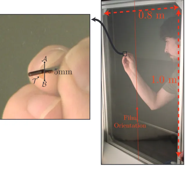
Figure 2.1: Pictures of the spiral experiment.Right: The whole experiment is
presented; the red line in the center of the picture is the universal orientation of the film. In this case, the initial incision has been made parallel to the film orientation.Left: Zoom centered on the initial incision, the points A, B, and T
Far from the edges of the thin sheet, we make a small straight cut with a knife,
typically of ∼ 5mm. We place a slim cylindrical1 in the incision perpendicular to
the plane of the film. Using this tool we nucleate and force to propagate a crack at point B, by pushing one lip of the initial incision. By continually doing this, a curved path appears. At the beginning of the experiment it is important to keep the tool closer to the crack tip than to the other end of the incision because this
asymmetry determines which crack will start to propagate (In Fig. 2.1 points T
and A respectively), however this will be important only while there is another po-tential nucleation point (In this case point A), and later in the experiment, it is not longer necessary.
Figure 2.2: In the figure we diagram the wide range of possibilities we have to
push the lip at the beginning of the experiment (red arrows), within rule R. In this case we only draw arrow close to point T to ensure that the propagation occurs at this point.
Note that we are careful to maintain the orientation of the film (the effect of
orien-tation will be discussed later in section2.6), so we use pieces from a single very
long rolled sheet and define a universal orientation across all the experiments.
1The shape of the tool is not be important in the fracture process, however it is important to use
Throughout the experiment, we move the blunt tool according to only the following rule: R:“always push the same lip”. This rule is rather loose, and leaves the free-dom to push anywhere in the lip as we illustrate in Fig.2.2.
However, following this process, we obtain a smooth crack path, a large spiral
which grows from a ∼ 10mm initial cut to a roughly ∼ 1m diameter spiral in only
2.5 turns.
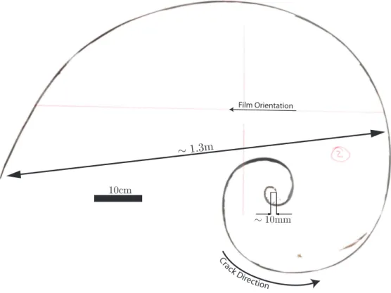
An example of the final tear is shown in the picture in Fig.2.3.
C ra
ck D irection Film Orientation
Figure 2.3: Picture of the final tear obtained. The external edge of the darker zone
2.2
Tool path dependence
Although the experiment is done by hand, the regularity of the resulting spiral
crack path in Fig.2.3is impressive because the movement of the tool has in fact
not impacted on the final shape, as we show now.
Illumined too
l Tip
Camera
Figure 2.4: Illustration for the tool tracking experiment
Starting with the same initial conditions, we have deliberately chosen to impose very different tool paths and velocities in two experiments (still following rule R).
The movement of the tool is tracked in images taken by a camera (see Fig.2.4).
In Fig.2.5we present the superposition of the tool positions and the contour (post-mortem) of the crack paths. The solid and dashed outlines are the crack paths, and the circle and squares are the respective tool trajectories (tool position at equal interval of time).
10[cm]
A
B
Figure 2.5: Tool Trajectories and its respective resultant crack paths.
Since the video gives us the position at equal intervals of time,∼ 0.5 second, the
distance between two consecutive points of the tool path is a measurement of its velocity. It is obvious that the tool paths were very different. However, as can be
seen in Fig.2.5the resulting crack paths are very similar and the small difference
at the end of the spirals (∼ 1cm)can be contrasted with the rapid growth of the
spiral: any small difference at the beginning is quickly amplified. The difference is
diameter.
This shows that the crack path is not determined by the will of the experimentalist, as one could imagine at first, but rather the system itself chooses the direction for crack propagation (as long as rule R is obeyed). In the rest of this chapter we try to explain this puzzling behavior.
2.3
Model
We now present a general model, for fracture propagation in a thin sheet loaded by a blunt object. Using simplifying assumptions for the mechanics of thin sheets
and fracture mechanics (Griffiths criterion [58] and the criterion of maximum
en-ergy release rate, initially postulated by Erdogan [59]), we find the condition for
crack propagation and predict the direction of the propagation. We will test our assumptions experimentally on a simple and more controlled configuration, and then we will compare the model and experiment in the case of spiral propagation.
2.3.1
Elastic Energy
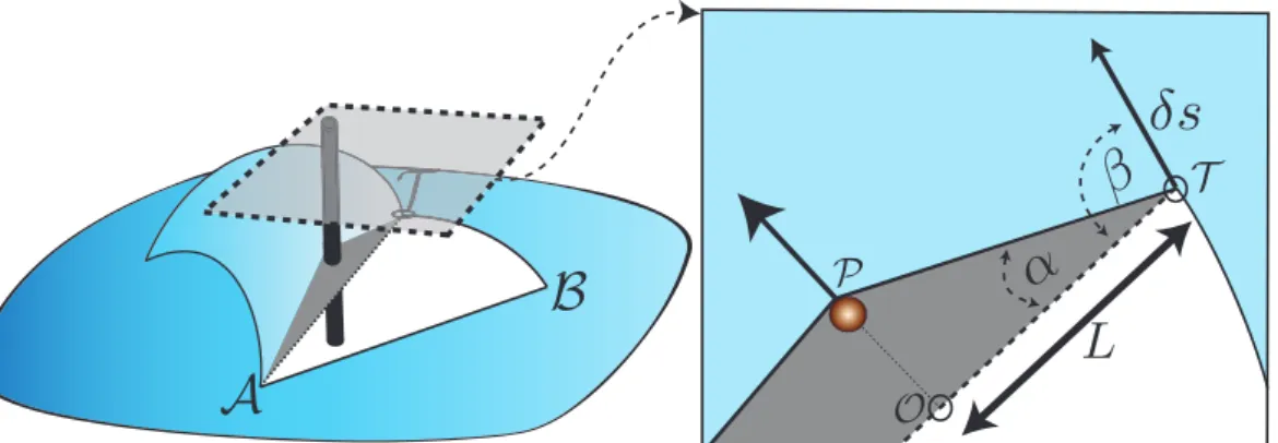
We identify a basic configuration of energy storage and release of energy, and the Spiral propagation is based on the repetition of this basic configuration throughout the experiment. Suppose that the crack has propagated a distance s from point B to point T , as illustrated in Fig.2.6. At this point in the experiment, the unstressed lip, segment AT , is pushed by moving the tool from point O to point P (see
illus-tration on the right in Fig.2.6). Consequently, the zone around the lip deforms and
stores elastic energy. The elastic energy in the system plays a key role for fracture
propagation, and we now characterize it experimentally.
2.3.1.1 Experimental Characterization of the Elastic Energy
In order to explore more easily the energy storage functionality in the system, we slightly modify the configuration observed in the spiral experiment. A straight cut 2L long is made in a thin brittle sheet of thickness t and Youngs modulus E (see
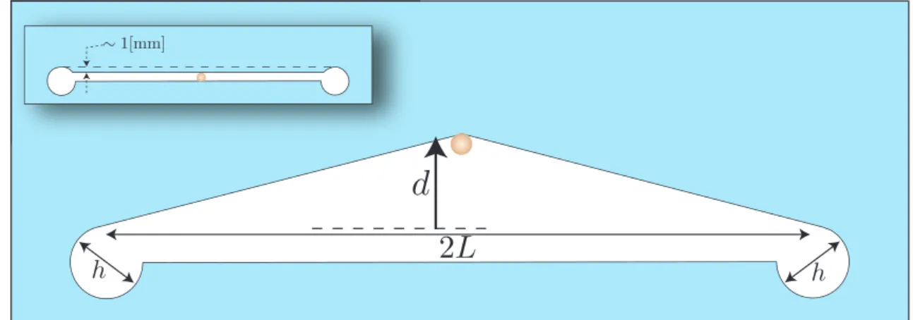
Fig.2.7). Both ends of the incision are blunted by small perforations (diameter of
h ∼ 4mm). This procedure, if performed carefully, leaves no appreciable notches in the film, reducing the probability of initiating fracture. The size of the perfora-tions is much smaller than that of the incision, in order to keep a constant length of the stretched lip. An illustration is presented in the inset in Fig.2.7.
Figure 2.7: Experimental diagram of the energy storage when a tool pushes a lip
of a thin sheet.
The force required to push the lip a distanced is measured in order to estimate
the elastic energy. If the tool is placed at the midpoint of the lip, owing to symme-try, the elastic contribution of the left and right sides will be the same. Using an
Instron 5865 electromechanical testing device, we slowly (speed∼ 1mm/s) move the tool perpendicularly to the lip and record the applied force with a load cell
In-stron 2525-807, with a limit load of100 N. Using this data and the size of the lip,
we determine the penetration angle α≈ d/L at equal intervals of time.
For this experiment we used materials of thicknesses of30, 50 and 90µm, with
Youngs modulus E = 2.9, 2.6 and 2.7GPa, respectively. We have measured the
force for initial cuts with lengths2L, of 6cm, 12cm, 18cm. The data, with
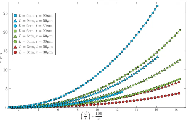
combina-tions of different film thicknesses and lengthsL of the lip, are presented in the plot of Fig.2.8.
Figure 2.8: Data from experiments with different lengths and different thickness
sheets. The penetration of the tool is given by the quantityd/L.
The curves stop for a given value ofd/L, for which fracture initiates from the blunt
for α observed in the spiral experiment, [6o, 12o], presented as a yellow region in
the graph in Figs.2.9and 2.10.
Since the sheet is very thin (compared to relevant lateral sizeL), we assume that
bending energy is negligible compared to stretching energy (see section C.1.2).
Since stretching energy is characterized by the combination Et, where E is the
Youngs modulus andt is thickness, we expect from the dimensional analysis that
the force obeysF = EtLφ(d/L), which can be developed for small values of d/L
intoF = EtL(d/L)n. And indeed, all the measured force collapsed whenF/EtL
is presented as a function ofd/L in Fig.2.9.
2 4 6 8 10 12 14 16 18 20 0.2 0.4 0.6 0.8 1 1.2 1.4 1.6 1.8 2 x 10⁻³
Figure 2.9: Data from experiments with different lengthsL and sheets with
The assumption of a mechanical response dominated by stretching energy2 in
[47,60] is therefore confirmed experimentally. An experimental measurement of
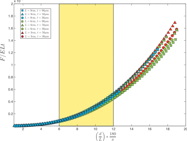
function φ(.) is obtained by plotting the same data in a semi-log plot (in Fig.2.10).
100 101
10−6 10−5 10−4 10−3
Figure 2.10: Experimental data presented in terms ofF/EtL versus the
penetra-tiond/L in a log-log plot.
In this graph, forces measured at small values of α < 1o are not represented for
two reasons. First we expect that in the early stage of indentation, bending
de-2Note however that in thin sheets theory, one usually use the opposite argument : if
stretch-ing energy is very costly, then the system tends to avoid stretchstretch-ing and stays close to isometric solutions, if possible. But this argument, at the base of [48], cannot hold here, since the loading condition clearly inevitably imposes some stretching.
formations exceed incipient stretching deformations and are therefore outside of
our theoretical description. Secondly, the experimental determination of zero ind
is difficult and modifies this part of the graph. In the inset on the top left corner
in Fig.2.8,we illustrate the initial configuration. A small flap is produced when the
initial cut is made. This flap has two consequences on the experimental mea-surements. One is that at the beginning of the experiment some bending related energy is measured, and the second effect is related to the position in which lip AB begins to be pushed. The procedure for setting the initial position is the fol-lowing: we manually approach the pushing tool to the lip until it is very close to the edge. Then, after the experiment is done, omit the part of the data where the force is small, because it means that there is no contact between the tool and the film. When this data is plotted in a log-log graph, they collapse in straight lines,
however for small values ofd/L not all the curves are straight. We attribute this to
the setting of the zero position. We have reset the zero for the curves that did not collapse completely. These curves are (L = 3cm t = 50µm), (L = 6cm, t = 90µm), (L = 9cm t = 90µm). The correction for these curves has been a shift in (d/L) in 0.04, which means a change of d in 1mm, 2.4mm and 3.6mm respectively. These changes are not small but are within the range of the experimental conditions. We
remark that doing this only affects the curves at very small values of(d/L) (in the
interval of 180π Ld between 1 and 2) and the data is unaffected in the fracture zone (in
yellow in Figs.2.9) and 2.10 The collapse over three decades of the force
mea-surements in Fig.2.10, demonstrates that the constitutive relation for the force in
this system can be very well approximated by:
F = 0.0266EtL! d
L "2.5
where the factor0.0266 and the power 2.5 are the average of the intersects and the
slopes of the respective parameters obtained fitting the curves in Fig.2.10. If we
now calculate the work done by the tool movement, we obtain the stored elastic energy,UE, in the system.
UE =
#
F δd = 0.0266EtL #
Lα2.5δα (2.2)
Finally a good approximation of the constitutive relation for the energy of the sys-tem is:
UE = 0.0076EtL2α3.5 (2.3)
The non-linear law in Eq. 2.3 cannot be explained by the usual linear elastic
re-sponse approach, which would lead to a quadratic energy dimensionally equiva-lent toEtL(d/L)2 ∼ EtLα2. It is not easy to include the non-linearities due to large
out-of-plane displacement. A first approach [3] is to consider that such a thin
ma-terial cannot convey compressive (negative) stresses, because they are released
by infinitely easy buckling. Following this idea, Audolys [47] estimated the
typi-cal strain in the system from the change in length of the pushed lip (initially with
lengthL and now L/ cos α) to be proportional to * ∼ α2. Since no compression is
transmitted, only a triangular zone (with sizeS ∼ Ld = L2α) is actually displaced
ahead of the pushing tool. The estimated stretching energy in the system would be proportional toEtS*2 = EtL2α5. The experimental data obtained in this section
disagrees with this result, the exponent being close to α3.5.
In a study of a similar problem, but in a different geometry, Vermorel et al [46]
have described the propagation of radial cracks when a cone pierces a thin sheet, leading to the propagation of several radial cracks. Propagation owes to the cone pushing on the lip in between consecutive cracks, leading to orthoradial tension *
similar to that in [47]. But the stored elastic energy was this time estimated from
the ideal 2D situation of a circle with radiusR subject to an orthoradial strain *.
The solution for 2D elasticity shows that strains decay like1/r2, where r is the
distance to the center of the disk, and that the disk radius increases by a distance d = R*. Finally, the energy is found Et(1 + ν)−1
(*R)2 . Although the interpretation
is not perfect because of radial geometry, we takeR as an equivalent of L, use
* ∼ α2, and find that this model leads to an energy scaling likeEtα4L2, with an
exponent4 which is closer to 3.5.
Energy functions proposed in [47] and [46] are built on the same hypothesis : only the lateral extensional stresses balance the pushing force in such a thin film. But
in [46] these extensional stresses are transmitted up to a characteristic distance
L, even if material points in this area are not directly pushed by the tool. This as-sumption is reasonable and gives a good approximation of the experimental law. We note that the experimental exponent is slightly smaller than predicted, which suggest that the assumption of infinitely thin sheet might not be completely valid.
We now turn to non symmetric loading, as depicted in Fig. 2.11.The energy is
the result of a spatial integration of the strain square, so that it is the sum of the integrals of the left and right sides respect to the tool. Nevertheless this does not necessarily mean that the energy from the left and the right have the same func-tionality as in Eq. (2.3), because the strains from left and right sides are coupled.
We have measured the force in a non-symmetric situation, as in Fig.2.11
Based on the results expressed in Eq. (2.1), we assume that the force has the
form, F = aEt $ L! d L "2.5 + L!! d L! "2.5% (2.4)
Figure 2.11: Non-symmetric experimental measure of force.
Wherea is a factor to be obtained from the data.
The combined nonlinear dependency on the two parameters,d/L and d/L!
makes it impossible to analyze this data in a dimensionless way, as we do in the
symmet-rical case. However, we present in the plots in Fig.2.12, how the quantity F/Et
behaves as a function ofL!
(d/L!
)n+ L(d/L)n, forn ∈ [1, 3] for 4 experiments, in a
50µm-thick sheet, made with different asymmetric positions of the tool and keep-ing the total length of the edge,L + L!
=const.
0 0.01 0.02 0.03 0.04 0.05 0.06 00 0.005 0.01 0.015 0.02 0.025 0 0.002 0.004 0.006 0.008 0.01
Figure 2.12: Force measurements in a non-symmetric experimental configuration.
Fig. 2.12, n = 2.5, shows us evidence to assume that it is possible to separate the energy in the contribution of the left and right side of the lip with respect to the tool, a simple verification is possible with a linear polynomial fit. In averaging the resulting slopes for the corresponding linear behavior, we obtain the empirical mechanical response: F = 0.0129Et $ L! d L "2.5 + L!! d L! "2.5% , (2.5)
If we compare Eqs. (2.1) and (2.5) we note that the factor in the first is twice that of the second expression. Indeed in the symmetrical case, both sides contribute in the same way, leading to a factor 2. Thus, we conclude that, at least in the regime where fracture occurs, it is possible to express the energy in the form of Eq. (2.4)
2.3.2
Fracture Propagation
Once we have an expression for the energy, we turn the discussion to model frac-ture propagation. We reformulate in a different way an argument equivalent to that
of [47]. Consider the example where the crack is at point T after it has propagated
a distances (see Fig.2.13(a)). As was done by Audoly et al. [47].,we define the
convex hull of the crack path. In this case it is the interior zone demarcated by the points A, B and T . In the previous section we have shown that the system is guided by stretching energy, and not bending. This implies that the tool will not induce fracture if it is placed within the convex hull (which is in Audolys work it is called the “soft zone”), but only bending of a flap. In contrast, if we move the tool outside of the convex hull, the energy in the system will dramatically increase, as
soft zone is called the active zone since it is where the tool is working. At some threshold value, the system cannot store any more energy and releases it, at the
cost of creating a new surface: the crack now moves from the point T to T!, and
we see that the elastic energy decreases in the process: the active zone transfers area to the soft zone (now defined as the area demarcated by the points A, B, T , T!, see Fig.2.13(b)).
L
L
!P
T
A
O
s
α
!α
B
!
d
(a) Geometry before fracture.
P
T
A
s
B
L! + δL ! L +δLO
!T
!δs
α! +δα !α + δα
β
!
d +
δ
!
d
(b) Geometry after the crack, of length s, propagates a distance δs.
Figure 2.13: Geometry of the system configuration.
In order to formalize the ideas presented above, we separate the fracture process in two stages:
1. Before rupture: The tool performs work by pushing the edge of the film
from point O to point P . Energy increases because of the stretching, which
is evaluated from the experimentally obtained expression in Eq. (2.3)
2. Rupture: Now that P is held fixed, we ask about crack propagation: does
the crack advance and to what position? .
Griffith’s approach [58,61] was to consider that the cracks position is the one that minimizes total energy
UT = UE + γts (2.6)
where we have noted UE the elastic energy, and γts is the energy associated
with a crack of length s, in a film of thickness t (γ is the work of fracture [61]).
This minimization is done with respect to the geometrical changes due to rupture
propagation of a small amount, from T to T!
. This modifies the valuesd, L, and
L!
(see Fig.2.13(b)). From the geometric dependence we obtain:
δUT = (∂dUE)L,L!δd + (∂LUE)d,L!δL + (∂
!
LUE)d,LδL!+ γtδs = 0 (2.7)
Where(∂xUE)y,z is the variation ofUE respect the variablex with y and z fixed.
Note that the force applied is connected with the energy by the relation ,F = ∂dUEd,ˆ
therefore the magnitude of the force is given by F = ∂dUE, so the equilibrium
equation is:
δUT = F δd + ∂LUEδL + ∂L!UEδL
!
+ γtδs = 0 (2.8)
2.3.2.1 Geometrical Variation
It is possible to calculate, from Fig.2.13(b), how much the system geometrically
changes when the fracture moves forward a length δs. A first result for δα is:
tan(−δα! ) ∼ −δα! = δssin β W −→ δα ! = −Wδs sin β (2.9)
whereW = L+L!
and β is the direction of the crack with respect to the unstressed
edge, segment AT in Fig.2.13(b).
Using the fact thattan(α + δα + δα!
) = (L tan α − δs)/(L − δs cos β), we solve for δα: δα = δs L cos α sin(α − β) − δα ! = δs L cos α sin(α − β) + δs W sin β (2.10) The distance δL! comes from: L! + δL! = L ! cos α! cos(α ! + δα! ) δL! = −δα! tan α! = δsL ! W tan α ! sin β = δsL W tan α sin β (2.11)
To calculate δL we use the fact that −δα!
( 1: L + L! − δs cos β L + δL + L!+ δL! = cos(−δα) ∼ 1 δL = −δs cos β − δs L W tan α sin β (2.12)
Finally, we calculate δd using (L tan α + δd)/(L + δL) = tan(α + δα). Directly we obtain:
δd = L sec2(α)δα + tan(α)δL (2.13)
After some algebra and using results from Eq. (2.9) and (2.10), we get δd changes
as a function of δs as:
δd = −δsL
!
2.3.2.2 Griffith’s criterion and second Variation of the energy
The first variational equation that represents equilibrium of the system in Eq. (2.8)
is Griffiths criterion. With the geometric relations obtained above, Eqs. (2.11),
(2.12) and (2.14), it may be written: ! −L ! WF − L W tan α (∂LUE − ∂L!UE) " sin β − ∂LUEcos β = −γt. (2.15)
where the left side of the equation is the energy release rate, which equals fracture energy when the crack propagates. We see that the energy released depends only on the direction β in which the crack propagates for a given loading condition (L, L!
, d and therefore F are fixed). Maximum release rate criteria establish that
the crack will choose the direction in which more energy is released. This implies the second variation:
∂ ∂β δU δs = ! −L ! WF − L W tan α (∂LUE − ∂L!UE) " cos β + ∂LUEsin β = 0 (2.16)
These equations can be written in a more compact way. Solving for ∂LUE in the
last term on the middle expression in Eq. (2.16) and replacing this result with the
corresponding term in Eq. (2.15) we obtain:
F = L
L! tan α (∂L!UE − ∂LUE) +
W
L!γt sin β (2.17)
If we use this result in Eq. (2.16) a second expression is obtained:
∂LUE = γt cos β (2.18)
This set of equations is the basis in our analysis to compute the fracture
param-eters. For a given position of the tool (set byL and L!
), in a given material (with
Youngs modulusE and fracture energy γ), we need three constitutive relations to
2.3.2.3 Fracture Propagation Law
We can now use our estimates for the force and elastic energy, to obtain the rules for the propagation of the crack in our configuration. From the results in section
2.3.1.1, we know that the dominant energy is stretching and it can be written as the sum of the contribution of the left and right sides, this isUE = Ul+ Ur:
UE = Ul+ Ur = aEt ! L!2! d L! "n + L2! d L "n" . (2.19)
The total force is:
F = ∂dUE = aEt & nL!! d L! "n−1 + nL! d L "n−1' = anEtL & 1 +! L L! "n−2' αn−1 (2.20)
Similarly, we obtain the other terms in Eqs. (2.17) and (2.18) ∂LUE = ∂LUr = −aEtL(n − 2)! d L "n = −aEtL(n − 2)αn (2.21) ∂LlUE = ∂L!Ul = −aEtL! (n − 2)! dL! "n = −aEtL! (n − 2)α!n (2.22)
We are interested in the critical value αc when the crack starts to propagate, and
the direction for the propagation, angle β. We begin by replacing Eqs. (2.20),
(2.21) and (2.22) in (2.17). This leads to:
anEtLαn−1(1 + ρn−2) = γt sin β (1 + ρ) + aEt(n − 2)Lαn+1ρ
where we have defined ρ= L/L’ a geometric parameter that is small if the tool is
close to the crack tip. Since we are working in the regime α ( 1, we neglect the
last term in Eq. (2.23), because of the high order of α. Eqs. (2.17) and (2.18) take the form:
anEtLαn−1(1 + ρn−2)
= γt sin β (1 + ρ) (2.24)
−a (n − 2) EtLαn = γt cos β (2.25)
We have two equations and two unknowns α and β. We first resolve β:
cot β = − (1 + ρ)
(1 + ρn−2)
(n − 2)
n α (2.26)
We know through experiments that the solutions for β must be close to π/2 so
cot β = tan(π/2 − β) ∼ π/2 − β, consequently Eq. (2.26) becomes:
β = π 2 + (1 + ρ) (1 + ρn−2) (n − 2) n α (2.27)
Using this result, we have for Eq. (2.24): αc = ! γt anEtL 1 + ρ 1 + ρn−2 "1/(n−1) (2.28) We now review the assumptions made to obtain the last two relations. The main requirement in our calculations is to have small angles α, α!
( 1 along the fracture process. However, this cannot be true if the tool is too close to points T or A in Fig. 2.13(a). The divergence when the tool approaches point T is explicit from
Eq. (2.27), however, it is a weak divergence due to the low exponent1/(n − 1) ≈
0.4. The failure of our approach when the tool is close to point A is observed in
Eq. (2.23), where a term of higher order in the angle α was neglected. Comparing
this term to the left side of the same equation, we obtain (for the validity of this approximation) the condition,
We have experimentally measured a typical value of αc ∼ 10o, if we plug this
value in Eq. (2.29) we obtain that the assumption is satisfied for ρ ! 4, which
impliesL ! 0.8W . Thus, the tool cannot be closer than a distance W/5 to point
A. Now, when we are moving the tool within the regionL ! 0.8W , we observe,
from Eqs. (2.28) and (2.27), that the factor(1 + ρ)/(1 + ρn−2) changes α and β no
more than 2 and 0.9 degrees, respectively, due to variations in ρ. Therefore, it is a good approximation to neglect ρ in relation Eqs. (2.27) and (2.28). It yields
αc = * γ anEL +1/(n−1) (2.30) β = π 2 + (n − 2) n α (2.31)
This result shows that α and β depends onL with a weak power. Thus, we
con-clude that the distance L is not important in crack growth, since, with some
re-strictions, α and β are fairly constant geometrical parameters.
By using the results from section 2.3.1.1, we expect a value of n ∼ 3.5, which
imply that Eqs. (2.30) and (2.31) take the form:
αc = * γ 3.5aEL +0.4 (2.32) β = π 2 + 0.4αc (2.33)
It is remarkable that the fracture process, despite large complex deformations, is completely characterized with these two geometrical expressions.
2.3.2.4 Model Confirmation
Eq. (2.32) establishes a threshold value for the angle α. The dependence on the
distanceL is rather weak, but we have designed a simple experiment to measure
In a50µm-thick sheet, we made a 23-cm-long incision. Because we want the crack to propagate only at one end, by making a small hole at the other end of the inci-sion, we geometrically avoid secondary nucleation.
With a high-definition video camera, we recorded the fracture process and mea-sured the critical value of the angle α (this is the value just before the crack
prop-agates) and studied how αc evolves with the distance between the tool and the
crack tip,L.
Figure 2.14: Critical value of penetration angle αc as a function of the
dimension-less quantity EL/γ plot with red dots. The black line corresponds to the linear fit
of the logarithmic rectification of the collected data.