Calibration of Wide Field Imagers - The SkyDICE Project

(1)

HAL Id: tel-00922070

https://tel.archives-ouvertes.fr/tel-00922070

Submitted on 23 Dec 2013

HAL is a multi-disciplinary open access archive for the deposit and dissemination of sci-entific research documents, whether they are pub-lished or not. The documents may come from teaching and research institutions in France or abroad, or from public or private research centers.

L’archive ouverte pluridisciplinaire HAL, est destinée au dépôt et à la diffusion de documents scientifiques de niveau recherche, publiés ou non, émanant des établissements d’enseignement et de recherche français ou étrangers, des laboratoires publics ou privés.

Calibration of Wide Field Imagers - The SkyDICE

Project

P.-F. Rocci

To cite this version:

P.-F. Rocci. Calibration of Wide Field Imagers - The SkyDICE Project. Instrumentation and Methods for Astrophysic [astro-ph.IM]. Université Pierre et Marie Curie - Paris VI, 2013. English. �tel-00922070�

(2)

THESE DE DOCTORAT

UNIVERSITÉ PIERRE ET MARIE CURIE

Spécialité: Physique

École doctorale : La Physique de la Particule à la Matière Condensée - ED389

réalisée

LPNHE

présentée par

Pier-Francesco ROCCI

pour obtenir le grade de :

DOCTEUR DE L’UNIVERSITÉ PIERRE ET MARIE CURIE

Sujet de la thèse :

Calibration of Wide Field Imagers: The SkyDICE Project

soutenue le 4 Novembre 2013

devant le jury composé de :

M. Massimo Della Valle Rapporteur

M. Laurent Derome

Rapporteur

M. Rémi Barbier

Examinateur

M. Pascal Vincent

Président de Jury

M. Nicolas Regnault

Directeur de Thèse

(3)

(4)

List of Figures

1.1 Map of the distribution of galaxies. Earth is at the centre, and each point represents a galaxy. Galaxies are coloured according to the ages of their stars. The outer circle is at a distance of two billion light years (Blanton M. and SDSS Collaboration 2008). . . . 4 1.2 This is a detailed all-sky picture of the Universe created from PLANCK data.

The image reveals old temperature ﬂuctuations that correspond to the seeds that after became galaxies, (Planck Collaboration et al. 2013a). . . . 5 1.3 Hubble diagram for 42 high-redshift SNe Ia from the Supernova Cosmology

Project, and 18 low-redshift SNe Ia from the Calan/Tololo Supernova Survey, after correcting both for the light-curve width-luminosity relation (Perlmutter et al. 1999). . . . 10 1.4 Planck TT power spectrum. The points in the upper panel show the

maximum-likelihood estimates of the primary CMB spectrum. The red line shows the best-ﬁt base CDM spectrum. The lower panel shows the residuals with respect to the theoretical model (Planck Collaboration et al. 2013b).. . . 12 1.5 The large-scale redshift-space correlation function of the SDSS LRGs sample.

The models are Ωmh2 = 0.12 (green), 0.13 (red), and 0.14 (blue), all with

Ωbh2 _{= 0.024 and n = 0.98. The magenta line shows a pure CDM model with}

Ωmh2 _{= 0.105 (Eisenstein et al. 2005).} _{. . . .} ₁₃

1.6 Spectra of SNe at maximum, three weeks, and one year after. The represen-tative spectra are those of SN1996X for type Ia, of SN1994I (left and centre) and SN1997B (right) for type Ic, of SN1999dn (left and centre) and SN1990I (right) for type Ib, and of SN1987A for type II (Turatto 2003). . . . 16 1.7 Calan/Tololo nearby Supernovae absolute magnitudes in V band, (a) - as

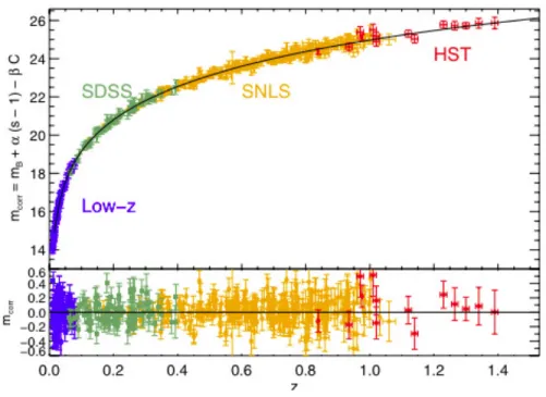
ob-served and (b) - after correction using the stretch parameter (Kim et al. 1997). 17 1.8 Hubble diagram of the same combined Low-Z, SDSS, SNLS and HST sample.

The residuals from the best ﬁt are shown in the bottom panel (Conley et al. 2011). . . . 19

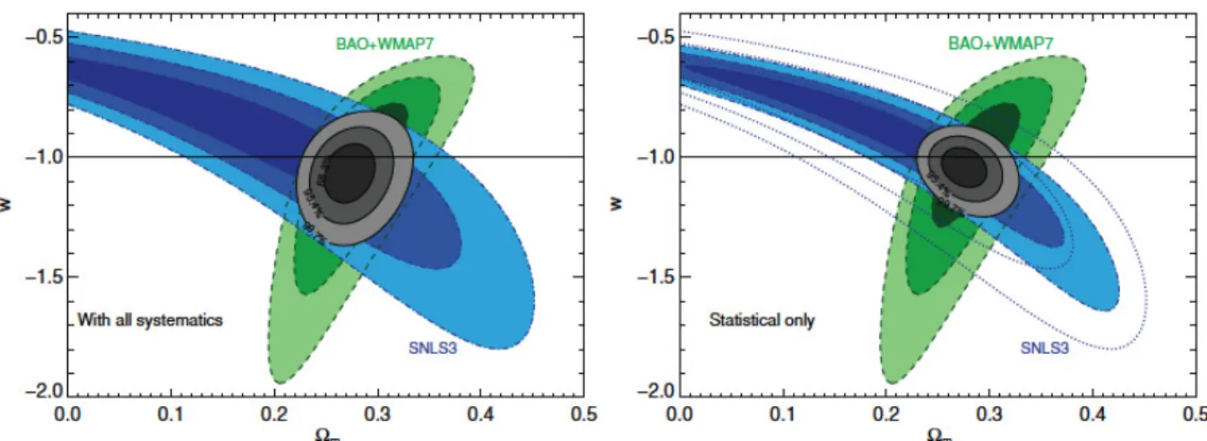
1.9 Statistical joint constraints on ΩM, w, ﬂat cosmological models (including

sys-tematics), CMB and BAO. The common contours (grey), constrain models close to a cosmological constant (Sullivan et al. 2011). . . . 20

(9)

LIST OF FIGURES

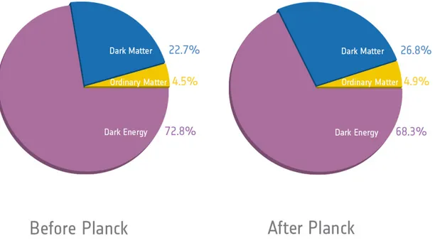
1.10 After Planck the baryonic matter counts for 4.9% of the total. Dark matter gives the rest 26.8%; this matter has only been detected indirectly by gravity eﬀect. The rest is composed of dark energy, that acts as a sort of an anti-gravity force (ESA/Planck Collaboration 2013). . . . 22 2.1 Arial view of the Siding Spring Observatory (SSO). SkyMapper is the one at

the top of the mountain in the centre (Siding Spring Observatory 2012). . . . 28 2.2 (Left) - Image of the SkyMapper telescope inside the dome. (Right) - Overview

of the optical design of the telescope. . . . 28 2.3 (Top) - Design of the SkyMapper imager system as seen from above.

(Bot-tom) - The CCD mosaic of the SkyMapper wide ﬁeld camera (Siding Spring Observatory 2012). . . . 30

2.4 Spectral response of SkyMapper science CCDs (Keller et al. 2007). . . . 31

2.5 SN Ia spectra at various redshifts. The shaded areas represent the imager passband. The distance estimate is generally chosen as the integral of the SN spectrum in the rest-frame B-band (Regnault 2013). . . . 32

2.6 NIST metrology chain (Regnault 2013). . . . 36

2.7 DICE metrology chain. . . . 37

3.1 Calibration variables monitored by DICE: passband normalizations and ﬁlter cutoﬀs. . . . 41 3.2 (Left) - Standard telescope illumination with a point source. (Right) - DICE

calibration beam (Regnault et al. 2012). . . . 42

3.3 Theoretical emission spectrum of a LED, see Schubert (2007). . . . 43

3.4 (Left) - MegaCam passband sampling by SnDICE. (Right) - SkyMapper sam-pling with SkyDICE LEDs. . . . 45 3.5 3-dimensional view of the illumination system. Two DC-MOTORS (1). The

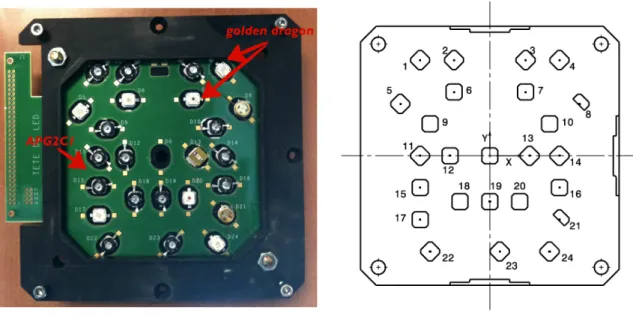
LED head (2). The front face of the device (3) displays 24 holes. The lens is mounted on a tip-tilt support (4). A linear motor (5) permits to shift the lens along the optical axis to adjust the focus. The lens arm is mounted on a manual X-Y plate (6). The planet LEDs are mounted on a board (7) placed behind the radiator (8). This board can slide linearly (9). A webcam (10) is mounted on the device. The LED and control photodiodes are mounted on two boards located on the back and front of the device. These board are connected to the backend electronics with two ﬂat cables (11). . . . 46 3.6 Overview of the LED head components. From left to right: (1) - planet lens

arm (2) lens; manual tiptilt lens support (3) manual XY support (4) -webcam (5) - planet focus DC motor (6) - LED head font panel (7) - photodiode board (8) - mask elements (9) - LED head elements (10) - holes (notice the 10 µm planet hole at the centre) (11) - LED board and radiator (12) - planet LED support (13) planet LED DC motor.. . . 47

3.7 Layout of the LED beam projection inside the DICE system. . . . 49

(10)

LIST OF FIGURES

3.9 Image taken from SnDICE data. We can clearly see the ghosts created by the primary and secondary reﬂections of the DICE source through optics and the ﬁlter of the CFHT telescope (Villa 2012). . . . 52 3.10 (Left) - SkyDICE main LEDs board with all 24 sources positioned. The hole

at the centre is the place of the artiﬁcial planet. (Right) - CAD drawing of the same circuit board. . . . 53

3.11 LED current generator and its feedback circuit.. . . 54

3.12 Overview of the SkyDICE DAQ system. We can recognise on the left the LED-head subsystem, and on the right the CLAP subsystem. Both are linked directly with the CICADA/TAROS DAQ system of the SkyMapper telescope. 56 4.1 (Left) - Test bench set up for spectrophotometric measurements, [A] the LED

head with its support and [B] the NIST photodiode support, then in [C] we can see the monochromator and in [D] the optical bench. (Right) - A real picture of the set up used to take spectra with the SkyDICE system. . . . 61 4.2 Eﬃciency η(λ) of the calibrated NIST photodiode (Hamamatsu S2281) used

for our measurements. The associated average error σ(λ)rel given by the NIST

is ∼ 0.2%. . . . 63

4.3 The plot shows the temperature of LEDs (PT1000), the average temperature of the test bench (LakeshoreA), and the temperature of the radiator (LakeshoreB) versus the time for all mini-maps taken in the run of 13th May 2012. As we aspect that the PT1000 and the Lakeshore probe are in good agreement. How-ever, values of the LakeshoreA are diﬀerent due to the temperature gradient inside dark-enclosure. . . . 65 4.4 We show all the temperatures reached during the full set of measurements for

all LEDs. The average range is from _{∼ 275 to ∼ 295 K.} . . . 66

4.5 An example of the beam map produced by the LED05 (hλpi = 512 nm) of

the SkyDICE source at room temperature. This is a row map where we only subtracted the dark current contribution from the NIST. . . . 66 4.6 (Left) - Optical design of a “Czerny-Turner”. The illumination source [A]

passes through the entrance slit [B]. The amount of light energy available for use depends on the intensity of the source in the space deﬁned by the slit. The slit is placed at the focus of a curved mirror [C]. The collimated light is diﬀracted from the grating [D] and then is collected by another mirror [E] which refocuses the light, now dispersed, on the exit slit [F]. A rotation of the dispersing element causes the band of colours to move relative to the exit slit, so the desired entrance slit image is centred on the exit slit. (Right) - The Diagram shows the typical triangle-shape transfer function for the Digikröm DK240 when the entrance slit and exit slit have the same aperture. . . . 69 4.7 Optical path of a monochromator. The mirror-grating system splits a

poly-chromatic point-like source in the diﬀerent wavelength components. . . . 70 4.8 (Left) - Single diﬀraction path. Here ǫ = θ is the grating inclination. (Right)

(11)

LIST OF FIGURES

4.9 Measurement of the monochromator transmission using the LED head itself (Guyonnet 2012). . . . 71

4.10 The ﬁgure presents the wavelength dispersion σmono and its temperature

de-pendence (Guyonnet 2012). . . . 73 4.11 The plot shows the temperature of LEDs (PT1000), the average

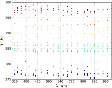
tempera-ture of the monochromator (LakeshoreA) and the temperatempera-ture of the radiator (LakeshoreB) vs. the time for all data taken in the last two runs of 26 and 27 April 2012. As we aspect the PT1000 and the LakeshoreB probe are in good agreement. However, the values of the LakeshoreA are slightly higher due to the temperature gradient. . . . 74 4.12 A plot with temperatures reached during the full set of spectra measured. The

average range is from _{∼ 275 to ∼ 300 K.} . . . 75 4.13 The correlation between the NIST and the oﬀ-axis control photodiodes slope

parameters for all studied LEDs.. . . 77 4.14 Linear ﬁt of the LED03 (395 nm). In the left is shown the data plus the ﬁt

obtained for the oﬀ-axis control photodiode, where in right side we presents the same results for the NIST photodiode. The two ﬁt are in good agreement. 78 4.15 For the red LED07 (625 nm), the result is in good agreement with what we

expect from the constructor data-sheets. Again the ﬂux decrease as the tem-perature increase. . . . 78 4.16 The same plot but for the LED05 (505 nm) at 1000 ADU. In that case it is

clear the strange behaviour that affect the LED at low current. The average flux increase as the temperature increase, instead decreasing as we expected from the data-sheets of the constructor. This effect disappears as soon as we augment the forward current of the device. . . . 79 4.17 We obtain the same result of LED05 for the LED24 (528 nm). Both are green

LEDs. . . . 79

4.18 Spectra of the UV LED03 (hλpi = 395 nm). The shape of the spectrum still the

same over the temperature, only the ﬂux decrease as the temperature increase. There is also al small shift on the central wavelength of the spectrum. . . . . 81

4.19 Another UV LED, this time the LED08 (hλpi = 320 nm) at diﬀerent

temper-ature. In this case the intensity of the current IN IST is really weak, ∼ 32 pA, as we expected for UV LEDs. This resulting on a really noisy spectrum. . . . 82

4.20 Spectra of the green LED05 (hλpi = 512 nm). This spectrum shows a small

bump at high wavelength, but in that case, due to a too few current, the LED works at sub-regime and shows an increase of the the measured current IN IST as the temperature increase. The wavelength is almost not shift along all temperatures range. . . . 83 4.21 The same LED05 but with an higher forward current. In that case the LED

works properly, showing a decrease of the ﬂux as the temperature increase.. . 83

4.22 Spectra of the red LED07 (hλpi = 625 nm). In that case not only the ﬂux

decrease, but it is evident that the all the spectrum shift with its central wave-length. . . . 84

(12)

LIST OF FIGURES

4.23 For spectra of the near-IR LED10 (hλpi = 810 nm) the behaviour is similar

to the red LED07 shown on ﬁgure 4.22. . . . 84 4.24 The plot represents the average wavelength computed from the NIST

photodi-ode measurements for the LED03. We ﬁt data with a linear law as a function of the temperature. The plot below show the small residual from the original data. . . . 87 4.25 Here is ﬁt drawn for the LED05. In that case the wavelength is weakly

depen-dents by the temperature. . . . 87

4.26 The ﬁt for the red LED07. The temperature dependence in that case are strong. 88

4.27 The ﬁt for the near-IR LED10. As the LED07 the temperature dependence is strong for near-IR LEDs. . . . 88

4.28 Digikrom240 transmission for the 3 gratings used in the measurements. . . . 90

4.29 Variance of the NIST eﬃciency η(λ). . . . 91

5.1 (Up) - The plot shows the dark corrected ﬂux contribution of the LED23

(hλpi = 464 nm), as a function of the temperature measured by the

Lakeshore-probe. The response is linear over all range of measured temperatures. The flux variations are due to readout noise coming from the not perfect shielded Keithley-NIST connection and from electromagnetic interference generated in-side the cable. (Bottom) - This figure shows the residual distribution from the linear law fit (red line). Here the RMS represents the relative uncertainties and its value is ∼ 4 · 10−4_. _{. . . .} ₉₆

5.2 The plot shows the dispersion of the ﬂux when the ﬂux follows a linear law only function of the Tled. The computed average value for all 23 LEDs is around

1.6 · 10−3_{. The second plot is the same when we do not consider the worst two}

LEDs. . . . 97 5.3 The two histograms represent the distribution of dispersion for all 23 LEDs

when we consider only the contribution from the temperature of LEDs Tled and the one from the backend electronics Tbe. In the first one we considered all LEDs, while in the second one at the bottom, we eliminated the worst two LEDs: LED09 and LED24. . . . 98 5.4 The two figures show the distribution of the flux dispersion evaluated taking

into account the temperatures Tled, Tbe and the variations of the voltage Vled. In the figure on the top we put all LEDs where in the figure on the bottom we eliminated (as figure 5.3) the two worst LEDs, LED09 and LED24. . . . 100 5.5 Time series of all measured parameters of LED09. We can recognise the NIST

flux, the photodiode flux, the LED and backend temperature and, finally, the LED current and the Voltage reference Vref used to calculate the LED and backend temperature. All flux, current and voltage values are normalised to one.101 5.6 Those two plots represent dispersion values calculated using the photodiode

model 5.5. The plot at the bottom is the same distribution when we discarded the three worst LEDs: LED09, LED24 and LED08 because of its photodiode problem. . . . 103

(13)

LIST OF FIGURES

5.7 This plot shows the final computed flux dispersion as a function of the wave-length. In particular we plotted the raw data (black diamond) versus the best result of the two different model. With green points the σf lux using the LED source model describes by equation 5.2, and with blue points using the off-axis control photodiode model with equation 5.5. . . . 104 5.8 This histogram shows the average flux dispersion for every LED beam map,

normalised by its reference central point. Even in that case the distribution is centred around 2.7_{· 10}−4_. _{. . . 105}

6.1 Synthetic spectra taken as an input for the model. . . . 110

6.2 Synthetic spectra taken as an input for the model. . . . 111

6.3 Recalibration parameters fs of all the spectra that were taken for one single

LED. For some LEDs, such as this one, one can measure a small residual dependency as a function of temperature. . . . 112 6.4 A spectrum aﬀected by a burst of noise. Before and after recomputing the errors.113

6.5 Fit of a SkyDICE spectrum (+residuals). . . . 114

6.6 Reconstructed LED spectra (from simulated data) (black). Eﬀect of a 1-nm error on the monochromator calibration, computed using the model derivatives w.r.t. the bench calibration systematics (dashed red line). . . . 115 6.7 Recomputed LED spectra (from simulated data) (black). Eﬀect on the

recon-structed spectra of a colour error in the determination of the NIST photodiode eﬃciency (dashed red). . . . 115 7.1 The ﬁgure shows the SkyDICE installation diagram for the LED-head and the

units of control. . . . 119 7.2 (Left) - Particular of the SkyDICE mounting system used to ﬁx the device

on the telescope’s enclosure. he mount is attached to a structure made of 3 ELCOM© _{bars, each of them ﬁxed on three points. (Right) - SkyDICE is placed} at 60◦ _{from zenith. We can recognise the backend box at the top of the device}

and all components mounted below the dome aperture. . . . 119 7.3 The pictures show the SkyDICE LED-head attached to the main arch of the

SkyMapper dome at the end of its installation in June 2012. . . . 120

7.4 The installation diagram for the CLAP system. . . . 121

7.5 A zoom of the CLAP installed in the mirror support system. We can recognise the small hole of the CLAP photodiode, and on the left a part of the primary mirror. . . . 121 7.6 (Top) - Shutter mode time sequence. (Bottom) - E-shutter mode time sequence.123 7.7 Origins and main reference frames for the telescope mount and primary mirror

(OAl, OAz), and for the dome position OD. . . . 125

7.8 Reference frame for the SkyDICE position. The origin ODICE (invisible in

(14)

LIST OF FIGURES

7.9 Because we could not scan all the primary mirror, we chose 4 positions A,B,C,D. These represent 4 diﬀerent conﬁguration between the telescope, the dome and the SkyDICE LED-head. Once we set up the altitude and the azimuth of the telescope, we move the dome to the decided position, then we centre the beam of SkyDICE with the focal plane of the telescope using the xy motors mounted on the LED-head. . . . 127

7.10 These are a set of images took using the LED05 (hλpi = 505 nm) with diﬀerent

exposures time. From top-left to bottom-right the filters used are: no filter with 3 s of exposure, g filter with 3 s, r filter with 15 s, and v filter with 100 s of exposure. Interesting features that emerged from images, are the diffraction patterns created by the dust and impurities on the CCDs focal plane and on the lens system. . . . 131

7.11 This is another image in false colours took with LED12 (hλpi = 850 nm) and

15 s of exposure. In that case the filter used was the z. We can notice the CCD grid reflected by the filter itself. . . . 131 7.12 Here we have the image of the focal plane illuminated by the artificial white

planet with 5 s of exposure without using filter. It is clearly possible the sum of the ghosts created by the internal reflections of the filter and the correction lenses system between the secondary mirror and the focal plane. . . . 133 7.13 The same picture but putting the filter g in front of the camera. Again the

ghosts are created by the lenses correction system and the ﬁlter. . . . 134 7.14 Dark dome illumination in ADU/s for the CCD ampliﬁers #33 and #26.

Without ﬁlter we can see that the contribution of the dome illumination is not trivial. . . . 138 7.15 The picture shows the preliminary result for the u, v ﬁlters transmission using

the data taken from the 30 June to the 2 July 2012 with the SkyDICE system. The CCD amplifier is the #33. . . . 141 7.16 The same analysis of figure 7.15 but for the g, r filters. The amplifier is the

#33.. . . . 142

7.17 The same analysis of figure 7.15 but for the i, z filters. Again the CCDs amplifier is the #33. . . . 143 7.18 Here we show the transmission parameters for the u, v filters outside the filters

passband. Even in that case the CCDs ampliﬁer was #33.. . . 144

7.19 Same plot of ﬁgure 7.18 but for the g and r ﬁlters. . . . 145

7.20 Again the same plot for ﬁlters i and z. . . . 146

8.1 Altered SkyMapper bands. Illustration of how we can alter the red front of the g-band and the blue front of the r-band, without displacing the other front. . 149 8.2 Correlation matrix of the calibration parameters for two hypotheses of the

NIST error budget. In both cases, the ﬁlter fronts are all positively corre-lated. This is because they all share the monochromator calibration uncer-tainty, which is the dominant contribution to the error budget. . . . 153

(15)

LIST OF FIGURES

8.3 Average of the calibration parameters reconstructed from 100 independent real-isations. All the parameters are well constrained, and no signiﬁcant bias can be detected on average. The error bars show the uncertainties as estimated from one single realisation. . . . 154 8.4 Statistical and systematic uncertainties on the measurement of the

SkyMap-per ﬁlter front displacements with the SkyDICE source, as a function of the precision of the calibration ﬂux measurements. . . . 155 8.5 Statistical and systematic uncertainties on the measurement of the SkyMapper

ﬁlter front displacements with the SkyDICE source, as a function of the number of runs (assuming a precision of the ﬂux measurements of 0.5%). . . . 156 8.6 Statistical and systematic uncertainties on the measurement of the SkyMapper

ﬁlter normalisation (relative to the r-band) as a function of the precision of the imager ﬂux measurements. . . . 158 8.7 Statistical and systematic uncertainties on the measurement of the SkyMapper

ﬁlter normalisation (relative to the r-band) SkyDICE source, as a function of the number of calibration runs (assuming a precision of the imager ﬂux measurements of 0.5%). . . . 159 A.1 3-dimensional model of the SkyMapper optics. In red we have represented the

SkyDICE beam used for our simulations. . . . 165 A.2 The plot represent the Root Mean Square (in pixel units) versus the position

of the secondary mirror (focus of the telescope). We found a value of _{∼ 1.5} pixels (22.5 µm) at a focus of +0.01702 m. . . . 169 A.3 Direct light illumination on the focal plane. We can see a vignetting eﬀect on

borders on the focal plane. . . . 170 A.4 Ratio of reﬂected light over direct light on the focal plane. The max value is

(16)

List of Tables

3.1 SkyDICE LEDs. The table shows the type, the central wavelength, the maxi-mum current and the corresponding SkyMapper ﬁlters. . . . 50

4.1 Typical SkyDICE LED currents and current upper limits. Iled is a nominal

current deﬁned for each LED. Isat is the current level at which control photo-diode starts to saturate. Finally IDICE

max is the maximum current the backend electronics can deliver to the LED (it varies from LED to LED, as it is a function of the serial resistor RL (see ﬁgure 3.11). (*) LED23 turned out to be faulty during the tests. . . . 60 4.2 SkyDICE photometric data sample taken during the 13 of May 2012 run. We

represent the current Iled used, the wavelength of the LEDs, the distance from the 0 point of the test bench z axis, points representing the rough centre of each beam (xref and yref) and the chosen range for the pico-ammeter. (*)LED23 is faulty. . . . 67 4.3 Wavelength dispersion oﬀset for the three grating conﬁguration measured at

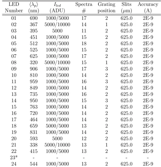
Ta= 25◦C with the their temperature dependence (Guyonnet 2012). . . . 72 4.4 SkyDICE spectroscopic data sample taken during the 26 and 27 of April run.

Iled is the nominal current in ADU for this run. Grating position is the chosen set up for the monochromator: in particular 1 = 1200 groove/mm, 1 = 600 groove/mm 1 = 300 groove/mm. (*)LED23 seems to be faulty. . . . 76 4.5 The table contains the slope parameters from the least-square ﬁt of the control

photodiode current and the NIST current, measured during the 26 and 27 of April run. The only missed value is the LED17 because of an instability of the flux at low forward current, and the LED14 because the fit did not converge. 80 4.6 The table show the full list of the slope parameter found using the linear fit

discussed in §4.5.2. . . . 86

4.7 Summary of the test bench systematics. . . . 91

5.1 LEDs list for the spare LED-head device used in this analysis with the Sky-DICE LEDs identiﬁcation. Imax represents the maximum DAC value available for the input current (corresponding to DACmax = 16384). Iled is the DAC current value used in this experience. . . . 94

(17)

LIST OF TABLES

7.1 Here we represent the whole set of data taken during diﬀerent data runs on summer 2012. Here the coordinates of azimuth, elevation and de-rotator are the reference values of the artiﬁcial planet used to centred the beam. During

each run this value slightly changed to centre the LED. . . . 129

7.2 This table is taken from the 30 June 2012 data sample. It shows the typical routine operation to take SkyDICE flat-fields for the UV LED03. The opera-tion is repeated for all 23 LEDs. In particular because the dome is not perfectly dark, at the start and at the end of the sample, we record different dome dark images to take into account the background level of the dome. . . . 136

7.3 Dome dark study of night and daylight along all the ﬁlters set for #33 and #26.139 8.1 Typical MegaCam and SkyMapper calibration runs. . . . 151

8.2 Systematics aﬀecting the ﬁnal SED measurements. . . . 160

A.1 SkyMapper main optical elements. . . . 167

A.2 SkyMapper focal plane elements. . . . 167

A.3 Materials and coating properties. . . . 168

A.4 Position on the focal plane of all reﬂections calculated using our ray-tracing model. . . . 171

(18)

per me si va ne la città dolente, per me si va ne l’eterno dolore, per me si va tra la perduta gente.

(D. Alighieri / Inferno - Canto III)

No hay méritos morales o intelectuales. Homero compuso la Odisea; postulado un plazo inﬁnito, con inﬁnitas circunstancias y cambios, lo imposible es no componer, siquiera una vez, la Odisea.

(19)

(20)

Remerciements

Tout d’abord je veux remercier mon Director de thèse, Nicolas Regnault, pour m’avoir suivi pendant tous les trois ans de travail jusqu’aux moment plus dure de la rédaction de ce manuscrit, et pour ses précieux conseils.

Un remercient à Laurent Le Guillou et Kyan Schahmaneche pour vôtres support scientiﬁque et aide pendant toutes les étapes du projet SkyDICE et pour m’avoir supporté en Australie. Je remercie tout l’ensemble du personnelle LPNHE sous le nom de son Director Reynald Pain. Un remerciement particulier au groupe Supernovae et à l’équipe technique du labora-toire qui ont permis la réalisation physique de SkyDICE (Merci Philippe Repain pour ton aide pendant l’installation!).

Je remercie encore le jury de thèse: les rapporteurs Massimo Della Valle et Laurent Derome, et les examinateurs Rémi Barbier et Pascal Vincent.

Un énorme merci à mes co-bureau présents et passés: Laura Zambelli (et ses plants), Au-gustin Guyonnet, Arnaud Canto, Mathilde Fleury (et son thé), Patrick El-Hage (et ses vidéos YouTube) et au dernier arrivé (University of Sussex Proud!) Ayan Mitra. Bonne chance à tous pour vos thèses et/ou vos carriers future.

Encore, Bonne Chance tous les souteneurs du 2013 pour vos PostDocs! Je voudrais même remercier le Pole Emploi français pour son soutien ﬁnancier pendant les prochaines mois (vive le chômage!).

Je veux remercier tous mes amis parisiennes avec les quels ma vie n’aurait pas été la même. Enﬁn tout cela n’aurait pas été possible sans le soutien de ma famille depuis le début et qui a été toujours présent dans cette aventure magniﬁque (Vi Voglio Bene!).

Un ringraziamento particolare va a te Mara, grazie per il tuo sostegno e la tua dolcezza, grazie per essermi stata vicino anche nei momenti più diﬃcili. Senza te quest’avventura non sarebbe stata la stessa.

(21)

Introduction

Between 1999 and 2001, three measurements changed Cosmology forever: the discovery of Cosmic Acceleration (Perlmutter et al. 1998;1999,Riess et al. 1998,Schmidt et al. 1998) in-dicated that the density of the Universe is dominated by some kind of repulsive Dark Energy (of unknown nature), the measurement of the ﬁrst acoustic peak in the CMB temperature anisotropy spectrum (de Bernardis et al. 2000) combined with the precise determination of

H0 (Freedman et al. 2001) gave strong constraints on the ﬂatness of space-time. These

mea-surements contributed to solve the persisting disagreements between the observations that were favouring a low density of matter, and theoretical motivations for a higher-density (criti-cal) Universe. It favoured the emergence of the Standard Model of Cosmology (Λ-CDM) that describes nearly all of today’s observations with only a handful of free parameters (Planck Collaboration et al. 2013b). Cosmology has now entered an era of precision measurements, and the goal of observations is now to hunt for “tensions” within the cosmological model.

The case of Supernova cosmology is very characteristic of this situation. The measure-ment of luminosity distances to SNe Ia as a function of their redshift allowed one to discover (with less than 100 supernovae) the acceleration of cosmic expansion. Today, SNe Ia are still the most sensitive probe to w, the Dark Energy equation of state parameter, and grow-ing number of SNe Ia are begrow-ing detected and studied by several Collaborations all over the world, in order to pin down the value of w, and to start ruling out Dark Energy models. The precision on w is now as low as 7% (Howell et al. 2009, Conley et al. 2011, Sullivan et al. 2011) with nearly 1000 SNe Ia in the Hubble diagram. Unfortunately, the measurement is now dominated by systematic uncertainties, the dominant source of systematics being the photometric calibration of the imagers used to measure the SN Ia ﬂuxes.

So, this work is about photometric calibration. This is a rather esoteric subject, which is seldom chosen by PhD students. But the thing is that, to improve on the current results, astronomers have no choice but to revisit the ancient calibration schemes. Since 2005, most Dark Energy Collaborations (with the invaluable help of the HST calibration program) have launched ambitious calibration eﬀorts, redeﬁned primary standards and metrology between those standards and their science images and push down their error budget well below 1% (e.g.Betoule et al. 2013). One suspect however, that these techniques, which rely on observa-tions of stellar calibrators, will not allow one to reach the calibration requirements of future surveys. For this reason, several groups in the world are working on experimental laboratory sources, that would allow one to inject very well characterised light into the telescope optics and derive, from these measurements, the telescope throughput as a function of wavelength. Since 2007, LPNHE cosmology group has been involved in the construction of a

(22)

spec-LIST OF TABLES

trophotometric calibration system for the last generation of wide ﬁeld imagers (Barrelet and Juramy 2008). In particular, the team has designed and built two devices: SnDICE (Super-novae Direct Illumination Calibration Experiment) and SkyDICE (SkyMapper Direct Illu-mination Calibration Experiment), the ﬁrst installed in the enclosure of the Canada France Hawaii Telescope (CFHT) on top of Mauna Kea, and the other in the dome of SkyMapper (Siding Springs Observatory, NSW, Australia).

This thesis is about SkyMapper. I started my PhD a few months after the SkyDICE project was funded. I was involved in nearly all stages of the project, in particular the integration and the calibration of the device on our test bench, as well as the installation and commissioning at Siding Springs. I then spent my third year analysing the commissioning data.

This memoir is organised as follows. In chapter 1 I described the standard model of Cosmology, with particular attention on the cosmological probes. I then (chapter2) describe the experimental context of this thesis: SkyMapper, the stellar calibration techniques and their limitations and I review the main instrumental calibration projects. In chapters 3 I discuss the design and implementation of the SkyDICE calibration source. Chapters 4, 5 and6present the central part of my work: the calibration and characterisation of the source on our spectrophotometric test bench. In chapter 7 I describe the installation of the device on site, and the pre-analysis of the commissioning data I did then. Finally, in 8, I present the method developed to constrain the SkyMapper passbands, from series of calibration observations, I test it on a simulation, and I estimate the uncertainties that will aﬀect our result.

(23)

Chapter 1 Modern Cosmology

At the end of the XIXth century our knowledge about the Universe outside the solar system was limited. Essentially our Galaxy, the Milky Way, was all we knew about Universe and Cosmology.

A theory to construct a real model of the Universe only came out with Einstein in 1917 and the publication of Theory of General Relativity (Einstein 1917); the ﬁrst model of the Universe studied by Einstein static and uniform. We have to wait for the work of Freidmann (Friedmann 1922), Lemaitre (Lemaître 1927), and later De Sitter (Einstein and de Sitter 1932), to see a ﬁrst theory where the Universe is dynamic and expanding. Around the same time Edwin Hubble made distance measurements of nearby galaxies, and discovered that Universe was in fact expanding. The publication of the famous Hubble’s law in 1929 (Hubble 1929), can be seen as the birth of modern Cosmology.

In the 1930s, observations of the nearby clusters by Zwicky (Zwicky 1937), proved that the galaxy halos were surrounded by something invisible, a type of matter that could only be inferred from its gravitational eﬀect; today, astronomers call this dark matter.

In 1998, two independent teams, working on supernovae projects, published observations of distant type Ia supernovae (Riess et al. 1998, Perlmutter et al. 1999), that indicated that the Universe was not only expanding but also that this expansion was accelerating. This milestones opened the way to the re-introduction of something that Einstein believed was his worst error: the cosmological constant.

After this brief history of modern cosmology we are going to focus on the basic concepts and equations used. In particular in §1.1 and §1.2 we describe the general principles behind modern Cosmology and the Λ-CDM model (also namely Concordance Model). Then, in the second part of the chapter, §1.3 and §1.4, we talk about Hubble’s law, the expansion and the discovery of acceleration. Moreover, we deﬁne the most important cosmological probes that astronomers use to constrain models, with particular attention on type Ia supernovae. Finally, in the third part of the chapter §1.5 and §1.6, we talk about the dark side of the Universe with the actual hypothesis for dark energy and dark matter.

(24)

1.1. THE COSMOLOGICAL PRINCIPLE

1.1 The Cosmological Principle

In 1543 Nicolaus Copernicus died and the same year one of the miles stone of human thinking the De Revolutionibus Orbium Coelestium were published. This book contained the seed of modern cosmology, known as the Copernican Principle. In a few words it says that our planet Earth is not at the centre of the Universe neither in a special position, this idea opened a new point of view about our Solar system and Universe.

To be more precise, Copernicus put the Sun at the centre of the Universe (and we know now this is not more true), but the power of this revolution was to eliminate the centrality of human being from science, in other words: there is not special observer. At the same time the works of Galileo and Newton, generalised in the past century with the introduction of General Relativity of Gravity, lead the way to the cosmology as we know it. A contemporaneous version of the Copernican Principle is the Cosmological Principle. In a simple way can be written as (Rowan-Robinson 1996):

«The Universe as seen by fundamental observers is homogeneous and isotropic»

This simple and pedagogic statement implies more profound meanings. First,

homoge-neous, means that every observer sees the same image of the Universe or, more simply, there

is no special places in the Universe (see ﬁgure1.1).

Figure 1.1: Map of the distribution of galaxies. Earth is at the centre, and each point

represents a galaxy. Galaxies are coloured according to the ages of their stars. The outer

circle is at a distance of two billion light years (Blanton M. and SDSS Collaboration 2008).

The second terms, isotropic, means that the Universe looks the same for every observer. There is not preferential direction or, in other way, an observation evidence taken from

(25)

1.2. SHAPE AND MATTER OF THE UNIVERSE

diﬀerent positions in the Universe must be the same. The two terms homogeneous and isotropic are distinct but related, a Universe that is isotropic from any two locations must also be homogeneous.

Until now the cosmological principle is consistent with observations taken in all the wavelengths, from radio to gamma rays. One of the best proof about the isotropy of the universe is the measurement of the Cosmic Microwave Background (CMB) done by COBE (Mather et al. 1990; 1994), WMAP and PLANCK (see ﬁg. 1.2). For example, the map from WMAP 7 years describes an uniform microwave background with a temperature of

T0 = 2.72548 ± 0.00057 K and oscillations less than 10−5 (Fixsen 2009).

Figure 1.2: This is a detailed all-sky picture of the Universe created from PLANCK data.

The image reveals old temperature ﬂuctuations that correspond to the seeds that after became

galaxies, (Planck Collaboration et al. 2013a).

1.2 Shape and Matter of the Universe

We now brieﬂy describe the metric in a homogeneous and isotropic Universe, the connection between geometry, mass and gravity (Einstein equations), and the solution of the Einstein equations within this metric, the Friedmann equations.

1.2.1 Friedmann-Lemaitre-Robertson-Walker Metric

The Friedmann-Lemaitre-Robertson-Walker metric (FLRW) describes an expanding, homo-geneous, isotropic Universe:

ds2 _{= −cdt}2+ a2_(t)   dr2 1 − kr2 + r 2_dθ2_{+ r}2_sin2_θφ2   (1.1)

where the spherical polar coordinates r − θ − φ describe the spatial dimensions, while the

(26)

1.2. SHAPE AND MATTER OF THE UNIVERSE

in space. The metric contains two unknown quantities, the scale factor a(t) (see §1.2.3) and the curvature k. The latter is a constant, derived from observations, and the metric is qualitatively diﬀerent depending on the value of k: every positive, zero or negative value corresponds to a possible geometry of the Universe,

k       

= 0, zero curvature: Euclidean Flat Universe

>0, positive curvature: Spherical Closed Universe <0, negative curvature: Hyperbolic Open Universe

(1.2)

Recent measurements of the cosmic background anisotropies (see (Hinshaw et al. 2012) or (Planck Collaboration et al. 2013b)), show that curvature k is close to 0. meaning our actual Universe has an euclidean geometry. This metric is one of the possible exact solutions of the Einstein’s ﬁeld equations.

1.2.2 Einstein Equations

Those equations are the mathematical core of the Theory of General Relativity (GR), pub-lished in 1915 (Einstein 1915). In GR the gravity is caused by the curvature of the space-time, curvature induced from the presence of matter in the space-time structure. One of the most important assumption of the theory is the Equivalence Principle, which is a generalisation of the the Galilean Principle of Relativity for non-inertial systems. Roughly speaking the principle says that the laws of physics experience by observers on a gravitational ﬁeld are the same of the those in inertial systems. One of the direct derivation of this postulate are the equivalence of the gravitational mass and the inertial mass. Coming back on Einstein equation, its last version can be written as:

Gµν = Rµν− 1 2gµνR− Λgµν (1.3) where Gµν is: Gµν = 8π c4GTµν (1.4)

On the right hand side Tµν is the energy-momentum tensor representing the properties

of matters in the Universe. On the left hand side is the expression of the geometry of the

space-time. More precisely, Rµν is the Ricci’s tensor, R is its trace and most important

gµν is the metric tensor directly connected with the metric geometry of space-time from the

equation ds2 _{= g}

µνdxµdxν. The symbol Λ is the cosmological constant; previously insert by

Einstein for the Steady-State model and then resurrected by modern Cosmology to account for the dark energy part (see §1.5).

Because of the lack of space in this work, we can schematically resume the meaning of this equation as follow (Liddle and Loveday 2009):

(27)

1.3. THE ACCELERATING UNIVERSE

as J. Wheeler said: Matter tells Space-Time how to curve, Space-Time tells matter how

to move.

One last point: eliminating matter (right hand side equal to zero) from the equation is not enough to remove curvature. This is consistent with the fact that from observations eﬀect of the gravitational ﬁeld still present in the vacuum around astronomical objects.

1.2.3 Friedmann-Lemaitre Equations

Before the discovery of the expansion of the Universe, Friedmann in 1922, and Lemaitre in 1927 found from Einstein equation a model of the Universe homogeneous, isotropic, and expanding. Two independent equations were found. The ﬁrst one derived from the (0, 0) component of the Einstein’s equations is:

˙a a !2 + k a2 = 8πG 3 ρ+ Λ 3 (1.5)

the second one comes from the (i, i) trace of the Ricci’s tensor: 2¨a a + ˙a a !2 + k a2 = −8πGp + Λ (1.6)

The terms ρ and p are respectively the density and pressure of the matter contained in the Universe. The ﬁrst equation describes the expansion rate of the Universe from the parameter ˙a. Combining the two equations1.5 and 1.6, we get the term of the acceleration of the Universe: ¨a a = − 4πG 3 (ρ + 3p) + Λ 3 (1.7)

Studying these equations for diﬀerent initial conditions we have three majors solutions:

a(t)          = ±t2/3 _{: matter domination} = ±t1/2 _{: photons domination} = e±t√Λ

3 : dark energy domination

(1.8) the scale factor a(t) is a function that describes the variations of the Universe at diﬀerent time of its history. In §1.3.1we are going to discover that this parameter is directly connected with the expansion rate of the Universe and the concept of redshift.

1.3 The Accelerating Universe

In 1917, Slipher discovered that galaxies were moving away us (Slipher 1917); but it was the work of Hubble (Hubble 1929), measuring the redshifts of nearby galaxies and discovering the law that has his name, to show the expansion of the Universe. Here we describe the Hubble’s law and redshift in §1.3.1, then we deﬁne cosmological parameters in §1.3.2. Finally we show recent progresses made by the discovery of the acceleration of the expansion done in 1998 by two teams leading by S. Perlmutter, and B. Schmidt, H. Riess.

(28)

1.3.1 Hubble’s Law

The linear proportion of the velocity recession of galaxies (and more generally for every astronomical object) and its distance is called the Hubble’s law and can be written as:

v = H0(t) · d (1.9)

where H0(t) = _a(t)˙a(t) is the expansion rate of the Universe. The constant is called Hubble’s

constant and it has an actual value of (Planck Collaboration et al. 2013b):

H0 = 68.0 ± 1.4 km · s−1· Mpc−1

By measuring the redshift of galaxies, Hubble was able to achieve this result, although ﬁnding a value for the Hubble constant 10 times larger than obtained by modern mea-surements. When a galaxy moves away from us, taking his spectra, we can see that the wavelength is stretched to the redder part of the spectrum. More precisely, if we call λe the

wavelength emitted by the source and λo the light seen by an observer, we have:

λo

λe − 1 =

a(to)

a(te) −

1 = z (1.10)

z is what we call the redshift of the object. Using the FLRW metric and co-moving coordi-nates (equation1.1), we can write the redshift as a function of the scale factor a(z):

a(z) = 1

z+ 1 (1.11)

this equation connects the scale factor a with the redshift of object. That means if we look an object at high redshift, for example z = 1, we are looking at the Universe how was in the past when its dimension were a = 1/2, roughly half the dimension of now. The scale factor says us that galaxies are not simply moving away from us only because of their proper motions, but it is all the space-time that is expanding.

1.3.2 Cosmological Parameters

Defining cosmological parameters is the first step towards testing theoretical model with the observational data. In this sense, cosmological parameters are a series of numbers which describe the detailed properties of our Universe such as density of matter. Using the Freid-mann equations 1.5, 1.6, 1.7, we can extract the definition of the first of these parameters, the critical density ρc:

ρc =

3H2

8πG (1.12)

the critical density is the density of the Universe that corresponds to a ﬂat euclidean geometry of the space-time, the actual value is ρc = 1.88 · 10−26h20· kg · m−3. Extracting the

(29)

diﬀerent components inside the Friedmann equation, we can redeﬁne the density parameter as follow:

ΩM =

ρM

ρc

(1.13) is the density parameter for matter components of the Universe,

Ωr =

ρr

ρc

(1.14) is the density parameter for the radiation component of the Universe,

ΩΛ =

Λ

3H2 (1.15)

is the density parameter for the cosmological constant (dark energy), and: Ωk =

ρk

a2_H2 (1.16)

describe the geometry of the Universe. Putting these four parameters together we can rewrite the Friedmann equation1.5 in a simple form:

1 + Ωk = ΩM + Ωr + ΩΛ = Ω (1.17)

This equation links explicitly the curvature of the Universe (the left hand side of the equation), with the density of single components (the right hand side). A universe with Ω = 1 is ﬂat, while Ω < 1 (Ω > 1) means a closed (open) Universe.

Another important parameter is the deceleration parameter that can be evaluated from Friedmann equations1.5 and 1.6 as:

q_{(z) = −} ¨a(t) a(t)H2 = 1 2 X i Ωi(z)[1 + 3wi(z)] (1.18)

We have rewritten the equation in terms of the new parameters Ω − i and wi, where the

latter is the equation of state (EoS) parameter w = p ρ.

1.3.3 The Acceleration of Expansion

The expansion rate of the Universe would be expected to be slowing down due to the grav-itational force between galaxies opposes to the expansion; in another way the expansion of the Universe should be decelerating. But in 90s, two diﬀerent groups published results about the studies of distant type Ia supernovae (Perlmutter et al. 1998; 1999, Riess et al.

1998, Schmidt et al. 1998), indicating that the expansion of the Universe was accelerating.

Measuring their redshift, they discovered that the supernovae were more faints (distant) that could be expected from a matter dominated Universe. This meant that at some point in the history of the Universe, the expansion has started to accelerate, see ﬁg. 1.3. As a consequence a Universe characterised by low density matter can be described in terms of

(30)

1.4. OBSERVATIONAL COSMOLOGY

an equation of state often expressed as p = w(z), where w(z) = w0 + wa(z)/(1 + z) (e.g.

Chevallier and Polarski 2001, Linder 2003)

consequence of that is a Universe with less matter density, lead by ﬂuid with negative pres-sure. Nowadays, comparing diﬀerent studies, we are able to say that almost ∼ 68, 3%(Planck Collaboration et al. 2013b), of the observable Universe is made by this unknown kind of en-ergy, namely dark energy.

Figure 1.3: Hubble diagram for 42 high-redshift SNe Ia from the Supernova Cosmology

Project, and 18 low-redshift SNe Ia from the Calan/Tololo Supernova Survey, after correcting

both for the light-curve width-luminosity relation (Perlmutter et al. 1999).

1.4 Observational Cosmology

To evaluate the view of the Universe that until now we have described, we need a way to measure its main parameters (§1.3.2), in order to confirm or reject the model. In these last years lots of progresses have been made in astronomy thanks to the advantage of the new satellites mission (i.e., HST, FERMI, PLANCK), and new sensible and big ground based telescopes (i.e., CFHT, VLT, KECK). In this section we show some of the most important probes in observational cosmology that put strong constrains in the Λ-CDM Model. In particular in §1.4.1 we describe the Cosmic Microwave Background, in §1.4.2 we talk about Baryonic Acoustic Oscillations, in §1.4.3 we briefly describe Large Scale Structures, and finally in §1.4.4 we talk about type Ia supernovae.

(31)

1.4.1 Cosmic Microwave Background (CMB)

The CMB is the relic radiation from the young Universe after the Big Bang. It is the dominant form of radiation in the present Universe and extremely close to isotropy, meaning that the radiation received from all direction is more or less identical. The origin of the CMB falls in the early stage of the evolution of the Universe, at a time corresponding to a

z ∼ 1000, when the temperature was cooling down suﬃciently to allow electrons and nuclei to bound together and form stable atoms; the average temperature was T ∼ 3000 K. At that time the Universe made the transition from opaque to transparent lead photons to propagate freely.

Technically, two separate physical processes were taking place around the formation of the CMB. One is recombination, and it is referred to the phenomena where electrons and nuclei could combine together and form atoms (t ∼ 380000 years after the Big Bang). The other eﬀect is the decoupling, and it is the time when the photons can ﬂy freely (it happened shortly after the recombination). The CMB was discovered in 1965 by Penzias and Wilson (Penzias and Wilson 1965, Wilson and Penzias 1967).

After the decoupling, the Universe continued to expand and photons continued to redshift. This expansion increased their wavelength about one thousand time, putting them into the microwave part of the electromagnetic spectrum. The spectrum of the CMB is a thermal spectrum with an actual temperature of roughly T0 ≃ 2.73 K, and it is one of the most

accurate measurements in Cosmology. One of the most important features of the CMB are the little ﬂuctuations in temperature. This anisotropies are the signature of the density ﬂuctuations of matter at the time of recombination and they are absolutely important in order to form the structures that we see in the present Universe. Since before the discovered by COBE in 1992 (Smoot et al. 1992), lots of studies have been made to constrain and understand anisotropies of the CMB. The main quantity to be measured is the radiation angular power spectrum, known as Cl:

Cl =

l

X

m=−l

|alm|2 (1.19)

where alm is the amplitude of spherical harmonics of temperature ﬂuctuations, describe

by the following equation:

∆T

T (θ, φ) =

X

m,l

almYlm(θ, φ) (1.20)

Because of the angular distribution of fluctuations depending on the geometry of the space-time, from the power spectrum we can have information about the real geometry of the actual Universe. The first peak of this spectrum (see fig. 1.4), corresponds to temperature fluctuations at the time of the recombination, and in the case of a flat Universe this peak is roughly at l ∼ 220 (l is the multipole momentum, connected with the angular size by

(32)

out with a value of the dark energy density parameter ΩΛ:

ΩΛ= 0.686 ± 0.020 (1.21)

Figure 1.4: Planck TT power spectrum. The points in the upper panel show the

maximum-likelihood estimates of the primary CMB spectrum. The red line shows the best-ﬁt base CDM

spectrum. The lower panel shows the residuals with respect to the theoretical model (Planck

Collaboration et al. 2013b).

1.4.2 Baryonic Acoustic Oscillations (BAO)

In the last years, the acoustic peaks in the cosmic microwave background power spectrum (BAO) have emerged as one of the strongest cosmological probes. Before of the period of decoupling, baryons (read neutrons, protons and electrons) interact strongly with photons, this interaction creating a strong pressure force. In the region of high matter density, gravity tried to draw the baryons in, while the pressure oﬀered a opposite force; these two factors created oscillations analogous to acoustic waves in a medium (while the radiation dominated, the speed of sound at these condition was really high v ∼ c/√3).

The scale of these oscillations is set by the acoustic horizon at the time of recombination, deﬁned as the co-moving distance travelled by sound waves between their creations and the time of the recombination, in numbers:

s= Z trec 0 cs(1 + z)dt = Z ∞ z cs H(z)dz (1.22)

(33)

where cs is the speed of sound deﬁned by the ratio from the baryonic density and the

density of photons at that time. Density perturbations on larger scales lead to oscillations in a longer time scale because of the proportional relation between their period and the length scale of the Universe. This relation shows us the fact that BAO can be used as “standard ruler” for length scale in cosmology: the length of this standard ruler can be measured by looking at the large distant scale structures as cluster of galaxies. In particular resolving the equation1.22 _{gives us where to look for them, at s ≃ 150 Mpc.}

Figure 1.5: The large-scale redshift-space correlation function of the SDSS LRGs sample.

The models are Ωmh2 = 0.12 (green), 0.13 (red), and 0.14 (blue), all with Ωbh2 = 0.024 and

n= 0.98. The magenta line shows a pure CDM model with Ωmh2 = 0.105 (Eisenstein et al.

2005).

Because of perturbations from dark matter are dominants compared to the baryonic ones, the peak in the correlation function is smaller and the acoustic signatures are fainter than the CMB signal. It is necessary to probe large structures of matter to ﬁnd this signature; the magnitude of this volume is 1h−3_Gpc3_.

The first detection of BAO peak was found in 2005 (Eisenstein et al. 2005). To measure BAO they used sample of Luminous Red Galaxies (LRGs) taken from the Sloan Digital Sky Survey (SDSS). The correlation function is showed in the fig. 1.5; in that figure we can see a little peak at 100h−1 _{Mpc. The position and intensity of the peak is strictly correlated to}

the density of baryons, meaning that it is possible to examine the amount of the ordinary matter in the Universe and, comparing that with theoretical predictions from WMAP 9 years (Hinshaw et al. 2012) and Hubble Space Telescope (HST) (Riess et al. 2009), we obtained a

(34)

value for the total density Ωtot:

Ωtot = 1.0027+0.0039−0.0038 (1.23)

This result is conﬁrmed by the seven years analysis of the SDSS data (Kazin et al. 2010). The detection of the BAO peak is direct demonstration of the Big Bang model and the early evolution of the Universe at the epoch of the recombination and decoupling; the value found from SDSS analysis is in accord with a z ≃ 1000.

1.4.3 Large Scale Structures (LSS)

The various forms of structures we observe today in the universe are collectively referred to LSS. Observations of these structures provide us important constrains on the cosmological model since they are believed to trace regions with over-density in the early Universe after the epoch of inﬂation. There are several ways to measure them, but the two most important are cluster counts and the weak gravitational lensing.

Galaxy Clusters

Clusters of galaxies have a long history as cosmological probes, beginning with the ﬁrst dis-covery of dark matter (Zwicky 1937), through study of cluster of galaxies, and then providing evidence for a low matter density distribution (White et al. 1993). These discoveries came from observations of the properties of individual systems. But we know now that also the population of clusters as a whole contains lots of cosmological information.

The number of galaxy clusters in the local Universe measures the size of the density perturbations on a scale corresponding to the cluster mass. The way on which the number of clusters change with distance give us the changing-rate of the density perturbations. This rate depends on the total density of matter, but also on properties of the dark energy. The measurement of the spatial density and distribution of galaxy clusters is sensitive to dark energy through the angular-diameter and distance-redshift relation. To do that astronomers use several observables, either separately or combined, to infer the number and galaxy cluster mass function: direct counting, through the X-ray emission of the hot cluster gas (Mantz et al. 2008), although Sunyaev-Zeldovich and optical surveys are also making signiﬁcant progress in that ﬁeld.

In the Λ-CDM model, the number density of dark halos as a function of redshift can be compared with the number obtained in the large cluster surveys. The relation between galaxies cluster and its mass distribution can be written as:

d2_N_(z) dzdΩ = dM(z) H(z) Z inf 0 f(O, z)dO Z inf 0 p(O|M, z) dn(z) dM dM (1.24)

where f(O, z) is the observable redshift dependent selection function, dn(z)/dM is the co-moving density of dark halos, and p(O|M, z) is the probability that a halo of mass M at redshift z is observed as a cluster with observable O. This equation is sensitive to cosmology by the co-moving element d2

M(z)/H(z) and the growth structure term dn(z)/dM, which

(35)

Gravitational Lensing

Another method to study the large scale structures as galaxy clusters is to use the well known gravitational lensing effect. The light deflection caused by the gravitational potential of the cluster of galaxies, creates a distortion of the images of galaxies behind the lens. This kind of distortion allows us to measure the geometry and, overall, the distribution of total dark matter with its evolution in time. The observed shape of distant galaxies become slightly distorted as light from them passes through foreground mass structures. The distortion pattern depends then on the distances to the source and lens as well as its mass, being thus both a geometrical (distance-redshift) and mass distribution probe. This lensing signal that induces an observable ellipticity (cosmic shear) in the background galaxies has been detected (Bacon et al. 2000,Hoekstra et al. 2006), and wide field galaxy surveys are now being carried out (e.g. Fu et al. 2008), to improve the quality of this cosmological probe.

1.4.4 Type Ia Supernovae (SNe Ia)

A supernova is the phenomenon that occurs when a star ends its life in a violent explosion. This is one of the most energetic events in the universe, creating a new short-lived object in the sky, that outshines its host galaxy during a time of few weeks (≈ 30 days). Supernovae play a central role creating elements heaver than F e, and distributing these elements through space; more important, their extreme intrinsic luminosity make supernovae observable up to cosmological distances and a standardisable object to constrain dark energy equation.

Historically, supernovae classification has been based on their spectral features. Minkowski divided them into two groups (Minkowski 1941), depending on the existence of hydrogen lines on their spectra at maximum light: type I supernovae do not show hydrogen lines, whether type II supernovae do. This division was later extended by Filippenko (Filippenko 1997) and Turatto (Turatto 2003), as it became noticeable that there were more spectral and pho-tometric differences inside each group (see fig. 1.6). Furthermore, SNe Ia present an overall homogeneous spectroscopic and photometric behaviour, contrary to the other types. Those evidences are connected with the different physical mechanisms of origin between the SNe Ia and all the other SNe.

Assuming that a supernova originates from a single stellar object, two physical mech-anisms can explain the observed energy amount: the release of the nuclear energy by an explosive reaction (thermonuclear supernovae), or a gravitational collapse of a massive star (> 8M⊙), through the creation of a neutron star or a black hole (core-collapse supernovae).

Type Ia Supernovae as Standard Candles

Observationally, SNe Ia are deﬁned as supernovae without any hydrogen lines in their spec-trum, but with a broad silicon absorption line, Si − II, at about 400 nm. The progenitor is believed to be a binary system in which a CO white dwarf (no hydrogen layer), accretes ma-terial from a companion star (SD, single degenerate system), or possibly another white dwarf (DD, double degenerate system). The process continues until the mass of the white dwarf approaches the Chandrasekhar limit, at which point a thermonuclear explosion is triggered.