Deep Learning Methods for MRI Spinal Cord Gray Matter Segmentation

affiliée à l’Université de Montréal

Deep learning methods for MRI spinal cord gray matter segmentation

CHRISTIAN SAMUEL PERONE Institut de génie biomédical

Mémoire présenté en vue de l’obtention du diplôme de Maîtrise ès sciences appliquées Génie biomédical

Mars 2019

affiliée à l’Université de Montréal

Ce mémoire intitulé :

Deep learning methods for MRI spinal cord gray matter segmentation

présenté par Christian SAMUEL PERONE

en vue de l’obtention du diplôme de Maîtrise ès sciences appliquées a été dûment accepté par le jury d’examen constitué de :

Pierre BELLEC, président

Julien COHEN-ADAD, membre et directeur de recherche Nikola STIKOV, membre

DEDICATION

This thesis is dedicated to my wife Thais and my family.

“A rationalist is simply someone for whom it is more important to learn than to be proved right; someone who is willing to learn from others - not by simply taking over another’s opinions, but by gladly allowing others to criticize his ideas and by gladly criticizing the ideas of others."

ACKNOWLEDGEMENTS

I’m thankful to my research advisor Prof. Julien Cohen-Adad who gave me the opportunity to join NeuroPoly lab and for his diligent guidance during all this period on this interdisciplinary field of neuroscience and medical imaging. It was a pleasure to learn countless concepts and I easily became an admirer of his hard work towards a greater good.

I would like to thank Prof. Nikola Stikov and Prof. Pierre Bellec for gently accepting be part of the committee of my thesis defense and reading my work. Your criticism will be greatly appreciated.

I’m also very grateful to Ryan Topfer for all the extensive revisions and the time invested into his careful analysis of all the articles presented in this work.

I’m also very thankful to Prof. Rodrigo C. Barros, Prof. Evandro Luis Viapiana, Roberto Silveira and Thomas Paula for all the recommendations and incentive before coming to Montreal.

I would also like to acknowledge the financial support from IVADO, RBIQ/QBIN and for the Polytechnique Montreal financial exemptions. These fundings were paramount for this research.

This entire adventure wouldn’t be possible without the support from all my colleagues of NeuroPoly who were very kind and helpful to me since the day I arrived. I would like to thank Aldo, Maxime, and Charley for the very fruitful collaboration and discussions on Machine Learning. I would also like to thank Harris, Atef for helping me with the abstract translation and Agah, Tommy, and Francisco for all the friendly help during my masters at NeuroPoly. I’m also thankful to Pedro Ballester for the amazing collaboration on domain adaptation and solid friendship.

I would also like to thank Nikola for the help with the organization of journal club, it was an amazing experience.

It is also important to mention all friends from the NeuroPoly lab that helped me during this masters as well: Alexandru, Nicolas, Souad, Gabriel, George, Nibardo, Stephanie, Sara, Dominique, Benjamin, Tanguy, Tung, Alexandros, François, Mathieu, Jerôme, Ariane, Mélanie and Oumayma.

RÉSUMÉ

La moelle épinière humaine, qui fait partie du système nerveux central, est la principale voie responsable de la connexion du cerveau et du système nerveux périphérique. On sait que la matière grise présente dans la moelle épinière est associée à de nombreux troubles neurologiques tels que la sclérose en plaques et la sclérose latérale amyotrophique.

L’IRM est souvent utilisée pour étudier les maladies neurologiques et surveiller leur évolution. À cette fin, la morphométrie extraite de la substance grise de la moelle épinière, telle que le volume de la substance grise, peut être utilisée pour identifier et comprendre les modifications tissulaires associées aux troubles neurologiques comme ceux mentionnés précédemment. Pour extraire des mesures morphométriques de la matière grise de la moelle épinière, une annotation (label) par voxel est requise pour chaque tranche du volume IRM. L’annotation manuelle ne peut donc pas être facilement implémenté dans la pratique en raison non seulement des efforts fastidieux nécessaires pour annoter manuellement chaque tranche d’un volume d’IRM, mais aussi du désaccord et des biais introduits par différents annotateurs humains. Toutefois, il existe de nombreuses méthodes semi-automatiques ou entièrement automatiques pour annoter chaque voxel, mais la plupart d’entre elles sont composées d’approches en plusieurs étapes pouvant propager des erreurs dans le pipeline, s’appuient sur des dictionnaires de données ou ne généralisent pas bien lorsqu’il y a des changements anatomiques. Il est bien connu que les techniques modernes basées sur l’apprentissage par la représentation et l’apprentissage en profondeur ont obtenu d’excellents résultats dans un large éventail de tâches allant de la vision par ordinateur à l’imagerie médicale.

Le programme de recherche de ce projet consiste à améliorer les résultats les plus récents des méthodes existantes au moyen de techniques modernes d’apprentissage en profondeur grâce à la conception, la mise en œuvre et l’évaluation de ces méthodes pour la segmentation de la substance grise de la moelle épinière. Dans ce projet, trois techniques principales ont été développées: en open source, comme décrit ci-dessous.

La première technique consistait à concevoir une architecture d’apprentissage en profondeur pour segmenter la matière grise de la moelle épinière et a permis d’obtenir de meilleures résultats comparé à six autres méthodes développées précédemment pour la segmentation de la matière grise. Cette technique a également permis de segmenter un volume ex vivo avec plus de 4000 tranches en fournissant au préalable et moins de 30 échantillons annotés du même volume.

La deuxième technique a été développée pour tirer profitnon seulement des données anotées, mais aussides données qui ne le sont pas (données non anotées) au moyen d’une méthode d’apprentissage semi-supervisée étendue aux tâches de segmentation. Cette méthode a apporté des améliorations significatives dans un scénario réaliste sous un régime de données réduit en ajoutant des données non annotées au cours du processus de formation du modèle.

La troisième technique développée est une méthode d’adaptation de domaine non supervisée pour la segmentation. Dans ce travail, nous avons abordé le problème du décalage de distribution présent sur les données IRM, qui est principalement causé par différents paramètres d’acquisition. Dans ce travail, nous avons montré qu’en adaptant le modèle à un domaine cible présenté au modèle sous forme de données non annotées, il est possible d’améliorer de manière significative la segmentation de la matière grise pour le domaine cible invisible. Conformément aux principes de la science ouverte pour tous (open science), nous avons ouvert toutes les méthodes sur des référentiels publics et en avons implémenté certaines sur la Spinal Cord Toolbox (SCT) 1_{, une bibliothèque complète et ouverte d’outils d’analyse pour l’IRM} de la moelle épinière. Nous avons également utilisé uniquement des ensembles de données accessibles au public pour toutes les évaluations et la formation de modèles, ainsi que pour la publication de tous les articles sur les revues en libre accès, avec une disponibilité gratuite sur les serveurs d’archives pré-imprimées.

Dans ce travail, nous avons pu constater que les modèles d’apprentissage en profondeur peuvent en effet fournir des progrès considérables par rapport aux méthodes précédemment développées. Les méthodes d’apprentissage en profondeur sont très flexibles et robustes. Elles permettent d’apprendre de bout en bout l’ensemble des pipelines de segmentation tout en permettant de tirer profit de données non annotées pour améliorer les performances du même domaine dans un scénario d’apprentissage semi-supervisé ou en tirant parti de données non étiquetées pour améliorer les performances des modèles dans des domaines cibles non vus. Il est également clair que l’apprentissage en profondeur n’est pas une panacée pour l’imagerie médicale. De nombreux problèmes demeurent en suspens, tels que le décalage de générali-sation toujours présent lors de l’utiligénérali-sation de ces modèles sur des domaines non vus. Un futur axe de recherche inclut le développement en cours de techniques pour éclairer les mod-èles d’apprentissage automatique avec paramétrisation d’acquisition IRM afin par exemple d’améliorer la généralisation du modèle à différents contrastes, ainsi que d’améliorer la vari-abilité inhérente de ces images due aux différentes machines et aux changements anatomiques. L’estimation de l’incertitude liée à la distillation des connaissances au cours des phases de formation des approches décrites dans ce travail constitue un autre domaine de recherche

potentiel. Cependant, les mesures d’incertitude font partie d’un domaine de recherche en cours d’évolution dans le Deep Learning. En effet la plupart des méthodes fournissant une approximation médiocre ou une sous-estimation de l’incertitude épistémique présente dans ces modèles.

L’imagerie médicale reste un domaine très difficile pour les modèles d’apprentissage automa-tique en raison des fortes hypothèses d’identité distributionnelle formulées par les algorithmes d’apprentissage statistique ainsi que de la difficulté à incorporer de nouveaux biais inductifs dans ces modèles pour tirer parti de la symétrie, de l’invariance de rotation, entre autres. Néan-moins, avec la quantité croissante de données disponibles, elles offrent de grandes promesses et gagnent lentement en robustesse pour pouvoir entrer dans la pratique clinique.

ABSTRACT

The human spinal cord, part of the Central Nervous System (CNS), is the main pathway responsible for the connection of brain and peripheral nervous system. The gray matter present in the spinal cord is known to be associated with many neurological disorders such as multiple sclerosis and amyotrophic lateral sclerosis.

Magnetic Resonance Imaging (MRI) is often used to study diseases and monitor the disease burden/progression during the course of the disease. To that goal, morphometrics extracted from the spinal cord gray matter such as gray matter volume can be used to identify and understand tissue changes that are associated with the aforementioned neurological disorders. To extract morphometrics from the spinal cord gray matter, a voxel-wise annotation is required for each slice of the MRI volume. Manual annotation becomes prohibitive in practice due to the time-consuming efforts required to manually annotate each slice of an MRI volume voxel-wise, not to mention the disagreement and bias introduced by different human annotators.

Many semi-automatic or fully-automatic methods exist but most of them are composed by multi-stage approaches that can propagate errors in the pipeline, rely on data dictionaries, or doesn’t generalize well when there are anatomical changes. It is well-known that modern techniques based on representation learning and Deep Learning achieved excellent results in a wide range of tasks from computer vision and medical imaging as well.

The research agenda of this project is to advance the state-of-the-art results of previous methods by means of modern Deep Learning techniques through the design, implementation, and evaluation of these methods for the spinal cord gray matter segmentation. In this project, three main techniques were developed an open-sourced, as described below.

The first technique is the design of a Deep Learning architecture to segment the spinal cord gray matter that achieved state-of-the-art results when evaluated by a third-party system and compared to other 6 independently developed methods for gray matter segmentation. This technique also allowed to segment an ex vivo volume with more than 4000 slices by just providing less than 30 annotated samples from the same volume.

The second technique was developed to take leverage not only of labeled data but also from unlabeled data by means of a semi-supervised learning method that was extended to segmentation tasks. This method achieved significant improvements in a realistic scenario under a small data regime by adding unlabeled data during the model training process. The third developed technique is an unsupervised domain adaptation method for segmentation.

In this work, we addressed the problem of the distributional shift present on MRI data that is mostly caused by different acquisition parametrization. In this work, we showed that by adapting the model to a target domain, presented to the model as unlabeled data, it is possible to achieve significant improvements on the gray matter segmentation for the unseen target domain.

Following the open science principles, we open-sourced all the methods on public repositories and implemented some of them on the Spinal Cord Toolbox (SCT) 2_{, a comprehensive and} open-source library of analysis tools for MRI of the spinal cord. We also used only public available datasets for all evaluations and model training, and also published all articles on open-access journals with free availability on pre-print archive servers as well.

In this work, we were able to see that Deep Learning models can indeed provide huge steps forward when compared to the previously developed methods. Deep Learning methods are very flexible and robust, allowing end-to-end learning of entire segmentation pipelines while being able to take leverage of unlabeled data to improve the performance for the same domain on a semi-supervised learning scenario, or by taking leverage of unlabeled data to improve the performance of models in unseen target domains.

It is also clear that Deep Learning is not a panacea for medical imaging. Many problems remain open, such as the generalization gap that is still present when using these models on unseen domains. A future line of research includes the on-going development of techniques to inform machine learning models with MRI acquisition parametrization to improve the generalization of the model to different contrasts, to the inherent variability of these images due to different machine vendors and anatomical changes, to name a few. Another potential area of research is the uncertainty estimation for knowledge distillation during training phases of the approaches described in this work. However, uncertainty measures are still an open area of research in Deep Learning with most methods providing a poor approximation or under-estimation of the epistemic uncertainty present in these models.

Medical imaging is still a very challenging field for machine learning models due to the strong assumptions of distributional identity made by statistical learning algorithms as well as the difficulty to incorporate new inductive biases into these models to take leverage of symmetry, rotation invariance, among others. Nevertheless, with the amount of data availability growing, they show great promises and are slowly gaining robustness enough to be able to enter in clinical practice.

TABLE OF CONTENTS DEDICATION . . . iii ACKNOWLEDGEMENTS . . . iv RÉSUMÉ . . . v ABSTRACT . . . viii TABLE OF CONTENTS . . . x

LIST OF TABLES . . . xiii

LIST OF FIGURES . . . xiv

LIST OF SYMBOLS AND ACRONYMS . . . xvi

CHAPTER 1 INTRODUCTION . . . 1

CHAPTER 2 LITERATURE REVIEW . . . 4

2.1 Medical review . . . 4

2.1.1 Spinal Cord . . . 4

2.1.2 Relevance of the Spinal Cord Gray Matter . . . 5

2.1.3 Magnetic Resonance Imaging (MRI) . . . 8

2.1.4 Magnetic Resonance Imaging of the Spinal Cord . . . 9

2.2 Machine Learning Review . . . 11

2.2.1 Supervised Learning . . . 11

2.2.2 Semi-supervised Learning . . . 13

2.2.3 Domain Adaptation . . . 15

2.2.4 Deep Learning . . . 17

2.2.5 Convolutional Neural Networks (CNN) . . . 19

2.2.6 Convolutional Neural Networks for Semantic Segmentation . . . 22

CHAPTER 3 OVERALL METHODOLOGY . . . 24

CHAPTER 4 ARTICLE 1: SPINAL CORD GRAY MATTER SEGMENTATION USING DEEP DILATED CONVOLUTIONS . . . 25

4.1 Article metadata . . . 26 4.2 Abstract . . . 26 4.3 Introduction . . . 26 4.4 Related Work . . . 29 4.4.1 Note on U-Nets . . . 31 4.4.2 Proposed method . . . 32 4.4.3 Datasets . . . 36 4.4.4 Training Protocol . . . 37 4.4.5 Data Availability . . . 41 4.5 Results . . . 41

4.5.1 Spinal Cord Gray Matter Challenge . . . 41

4.5.2 Ex vivo high-resolution spinal cord . . . 42

4.6 Discussion . . . 47

4.7 Acknowledgments . . . 48

4.8 Author Contributions . . . 48

4.9 Additional Information . . . 48

CHAPTER 5 ARTICLE 2: DEEP SEMI-SUPERVISED SEGMENTATION WITH WEIGHT-AVERAGED CONSISTENCY TARGETS . . . 49

5.1 Article metadata . . . 49

5.2 Abstract . . . 50

5.3 Introduction . . . 50

5.4 Semi-supervised segmentation using Mean Teacher . . . 51

5.4.1 Segmentation data augmentation . . . 54

5.5 Experiments . . . 55

5.5.1 MRI Spinal Cord Gray Matter Segmentation . . . 55

5.6 Related Work . . . 57

5.7 Conclusion . . . 57

5.8 Acknowledgements . . . 57

CHAPTER 6 ARTICLE 3: UNSUPERVISED DOMAIN ADAPTATION FOR MEDI-CAL IMAGING SEGMENTATION WITH SELF-ENSEMBLING . . . 58

6.1 Article metadata . . . 59

6.2 Abstract . . . 59

6.3 Introduction . . . 59

6.5 Semi-supervised learning and

unsupervised domain adaptation . . . 65

6.6 Method . . . 66

6.6.1 Self-ensembling and mean teacher . . . 66

6.6.2 Adapting mean teacher for segmentation tasks . . . 68

6.6.3 Model architecture . . . 70

6.6.4 Baseline employed . . . 70

6.6.5 Consistency loss . . . 71

6.6.6 Batch Normalization and Group Normalization for domain adaptation . . . 72

6.6.7 Hyperparameters for unsupervised domain adaptation . . . 73

6.7 Materials . . . 74

6.8 Experiments . . . 74

6.8.1 Adapting to different centers . . . 74

6.8.2 Varying the consistency loss . . . 77

6.8.3 Behavior of Dice loss and thresholding . . . 77

6.8.4 Training stability . . . 77

6.9 Ablation studies . . . 78

6.9.1 Exponential moving average (EMA) . . . 78

6.10 Domain shift visualization . . . 80

6.11 Conclusion and limitations . . . 81

6.12 Source-code and dataset availability . . . 82

6.13 Acknowledgments . . . 82

6.14 Article Appendix: Extended visualizations . . . 83

CHAPTER 7 GENERAL DISCUSSION . . . 84

CHAPTER 8 CONCLUSION, LIMITATIONS AND RECOMMENDATIONS . . . 85

LIST OF TABLES

Table 2.1 The relative proton densities and intrinsic T1 and T2 times. . . 9 Table 2.2 Summary of the available methods for spinal cord gray matter segmentation. 23 Table 4.1 A summary of the acquistion parameters from each site. Adapted from [2]. 25 Table 4.2 Parameters of each compared method for the spinal cord gray matter

segmentation. . . 36 Table 4.3 Training protocol for the Spinal Cord Gray Matter Challenge dataset. . 38 Table 4.4 Data augmentation parameters used during the training stage of the

Spinal Cord Gray Matter Challenge dataset. . . 38 Table 4.5 Comparison of different segmentation methods that participated in

the SCGM Segmentation Challenge against each of the four manual segmentation masks of the test set. . . 39 Table 4.6 Training protocol for the ex vivo high-resolution spinal cord dataset. . . 40 Table 4.7 Data augmentation parameters used during the training stage of the ex

vivo high-resolution spinal cord dataset. . . 40

Table 4.8 Description of the validation metrics. Adapted from the work [2]. . . 44 Table 4.9 Quantitative metric results comparing a U-Net architecture and our

proposed approach on the ex vivo high-resolution spinal cord dataset. . 46 Table 5.1 Result comparison for the Spinal Cord Gray Matter segmentation

challenge using our semi-supervised method and a pure supervised baseline. . . 56 Table 6.1 Evaluation results for domain adaptation in different centers. . . 76 Table 6.2 Results on evaluating on center 3. The training set includes centers 1

and 2 simultaneously, with unsupervised adaptation for center 3. . . 78 Table 6.3 Results of the ablation experiment for the domain adaptation approach. 79

LIST OF FIGURES

Figure 2.1 Diagram of the human spinal cord showing its segments. Source: Cancer

Research UK / Wikimedia Commons. CC BY-SA license. . . 5

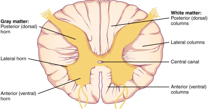
Figure 2.2 Anatomical cross-section of the spinal cord. Source: OpenStax Anatomy and Physiology, CC-BY license. . . 6

Figure 2.3 A histology slice of the spinal cord showing a clear tissue differentiation between myelinated white matter and gray matter. Best viewed in color. Source: OpenStax Anatomy and Physiology, CC-BY license. . . 7

Figure 2.4 Unnormalized MRI image intensity distributions for each center using axial slices from the Spinal Cord Gray Matter Segmentation Chal-lenge [2] dataset. The x-axis represent the MRI intensities and the y-axis represents the intensity distribution. Best seen in color. . . 10

Figure 2.5 A random axial slice from a random selected subject of the Spinal Cord Gray Matter Segmentation Challenge [2]. This image was produced by a 3D multi-echo gradient-echo sequence using a resolution of 0.25x0.25x2.5 mm on a 3T Siemens Skyra machine. The spinal cord is shown inside the green rectangle. . . 11

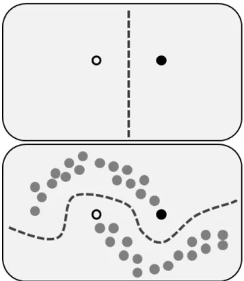
Figure 2.6 Top panel: decision boundary based on only two labeled examples (white vs. black circles). Bottom panel: decision boundary based on two labeled examples plus unlabeled data (gray circles). Source: Techerin, Wikimedia Commons, CC-BY-SA license. . . 16

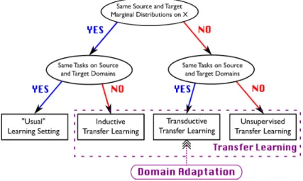
Figure 2.7 Distinction between usual machine learning setting and transfer learn-ing, and positioning of domain adaptation. Source: Emilie Morvant, Wikimedia Commons, CC-BY-SA license. . . 17

Figure 2.8 Network graph for a (L + 1)-layer perceptron. . . 19

Figure 2.9 (No padding, unit strides) Convolving a 3 ◊ 3 kernel over a 4 ◊ 4 input using unit strides (i.e., i = 4, k = 3, s = 1 and p = 0). Source: Vincent Dumoulin et al. [4], MIT license. . . 20

Figure 2.10 Architecture of a traditional convolutional neural network. . . 21

Figure 2.11 Illustration of a convolutional layer. . . 21

Figure 2.12 Illustration of a pooling and subsampling layer. . . 22

Figure 4.1 In vivo axial-slice samples from four centers that collaborated to the SCGM Segmentation Challenge . . . 28

Figure 4.3 Architecture overview of the proposed spinal cord gray matter segmen-tation method. . . 34 Figure 4.4 Training pipeline overview of spinal cord gray matter segmentation

method. . . 34 Figure 4.5 Qualitative evaluation of our proposed approach on the same axial slice

for subject 11 of each site. . . 42 Figure 4.6 Test set evaluation results from the SCGM segmentation challenge for

each evaluated metric. . . 43 Figure 4.7 Qualitative evaluation of the U-Net and our proposed method on the

ex vivo high-resolution spinal cord dataset. . . 45

Figure 4.8 Lumbosacral region 3D rendered view of the ex vivo high-resolution spinal cord dataset segmented using the proposed method. . . 46 Figure 5.1 An overview with the components of the proposed semi-supervised

method based on the mean teacher technique. . . 54 Figure 6.1 Samples of axial MRI from four different centers that participated in

the SCGM Segmentation Challenge. . . 61 Figure 6.2 MRI axial-slice pixel intensity distribution from four different centers. . 62 Figure 6.3 Data augmentation result of random MRI axial-slices samples from the

SCGM Segmentation Challenge. . . 68 Figure 6.4 Overview of the proposed domain adaptation method. . . 69 Figure 6.5 Data augmentation scheme used to overcome the spatial misalignment

between student and teacher model predictions. . . 69 Figure 6.6 Overview of the data splitting method for training machine learning

models. . . 75 Figure 6.7 Per-epoch validation results for the teacher model at center 3 with

cross-entropy as the consistency loss. . . 79 Figure 6.8 Execution of t-SNE algorithm for two different scenarios. Best viewed

in color. . . 80 Figure 6.9 Extended visualization based on t-SNE embedding from the domain

LIST OF SYMBOLS AND ACRONYMS

CNS Central Nervous System MRI Magnetic Resonance Imaging OSI Open Systems Interconnection CSA Cross-Sectional Area

EDSS Expanded Disability Status Scale SCGM Spinal Cord Gray Matter

NLP Natural Language Processing CNN Convolutional Neural Network RNN Recurrent Neural Network

IID Independend and Identically Distributed ERM Empirical Risk Minimization

CPG Central Pattern Generator ALS Amyotrophic Lateral Sclerosis MS Multiple Sclerosis

ERM Empirical Risk Minimization GAN Generative Adversarial Networks MLP Multi-Layer Perceptron

SGD Stochastic Gradient Descent FCN Fully Convolutional Network ASPP Atrous Spatial Pyramid Pooling

CHAPTER 1 INTRODUCTION

Neuroscientists usually divide the CNS into brain and spinal cord. The human spinal cord, responsible for connecting the brain and peripheral nervous system, is nearly as thick as an adult’s little finger and has two basic types of nervous tissues: gray matter and white

matter [5]. It is known, from histopathological studies [6], that tissue changes on the Spinal

Cord Gray Matter (SCGM) and white matter are related to a wide spectrum of neurological conditions.

Non-invasive imaging techniques such as MRI, that takes leverage of the nuclear magnetic resonance phenomenon through the use of strong magnetic fields and magnetic field gradients to provide spatial signal location, are usually employed to assess the spinal cord tissues such as the aforementioned gray matter and white matter.

In the last two decades, many semi-automated segmentation methods have been proposed for the estimation of the cord Cross-Sectional Area (CSA), however, individual gray matter tissue analysis cannot be individually assessed using only the CSA [7]. Given the significance of the spinal cord gray matter tissue analysis, which was found to be the strongest predictor of the Expanded Disability Status Scale (EDSS) in multiple sclerosis among many other metrics such as brain gray matter, brain white matter, FLAIR lesion load, T1-lesion load, and other metrics [8], the segmentation of the spinal cord gray matter became of greater importance due to its clinical relevance.

The manual annotation of the spinal cord gray matter is, however, very time-consuming even for a trained expert. The main properties that make the SCGM area difficult to segment are: inconsistent intensities of the surrounding tissues, image artifacts and pathology-induced changes in the image contrast [9]. There are also many other factors contributing to the complexity of the task, such as disagreement between different annotators, bias introduced by different annotators, different voxel sizes, lack of standardization protocols, among others. Therefore, a fully-automated procedure for the SCGM segmentation is paramount to provide means for studies that require automatic metrics extraction, tissue analysis, lesion detection, disorder detection, among others.

Recently, many methods have been proposed for the spinal cord gray matter segmentation [2,7, 10–16]. The scientific community, including our laboratory, recently organized a collaboration effort called “Spinal Cord Gray Matter Segmentation Challenge” (SCGM Challenge) [2], to assess the state-of-the-art and compare six independently developed methods on a public dataset created through the collaboration of four internationally recognized research groups

(University College London, Polytechnique Montreal, University of Zurich and Vanderbilt University), providing a ground basis for method comparison that was previously unfeasible due to the lack of standardized datasets.

In the past few years, we were able to witness the unprecedented pace to which Deep Learning [17] methods had evolved. Since the seminal work of the AlexNet [18], the research community embraced the successful Deep Learning methods and developed many state-of-the-art techniques that became pervasive across a wide range of tasks such as image classification [19], semantic segmentation [20], speech recognition [21] and Natural Language Processing (NLP) [22], to name a few.

A recent survey [23] that analyzed more than 300 papers from the field of medical imaging, showed that Deep Learning techniques became pervasive in the entire field of medical image analysis, with a rapid increase in the number of publications between the years of 2015 and 2016. The survey also found that Convolutional Neural Network (CNN) were more prevalent in the medical image analysis, with Recurrent Neural Network (RNN) gaining more popularity. Although the large success of Deep Learning has attracted a lot of attention from the community, it is clear that Deep Learning also poses some unique challenges such as high sample complexity, meaning that the amount of labeled data that these techniques usually require to train a reasonable classifier is very high. Another challenge that is still open is how to handle the domain shift that is present in many domains and especially in medical imaging due to the variability of protocols, acquisition devices, and human anatomy. Machine Learning techniques that follow the Empirical Risk Minimization (ERM) principle, often show a poor generalization performance when a trained model is evaluated on data from a different distribution, mainly because of the strong Independend and Identically Distributed (IID) assumption held by the ERM learning principle.

The first goal of this work is to show how Deep Learning methods can improve on the current state-of-the-art for the SCGM segmentation, through an extensive evaluation and comparison with other independently developed methods. The second goal is to show that even though Deep Learning has a high sample complexity, this can be alleviated through the use of semi-supervised learning techniques. The third goal is to show how Domain Adaptation techniques can be used to partially mitigate the poor generalization performance on unseen data. The fourth and last goal, in the spirit of Open Science principles, is to implement, document and test all developed software and make it available to the general public under a permissive open-source license at zero cost.

This thesis is organized as follows. In Chapter 2, we present a short critical literature review of previous works as well as a review of some concepts important to the themes that will

be developed later. In Chapter 3 we present an overall methodology and the main research questions guiding the research agenda. In Chapter 4, we present the first article where we develop a supervised end-to-end approach to the spinal cord gray matter segmentation using dilated convolutions; in Chapter 5 we present the second article where we develop a semi-supervised approach to the spinal cord gray matter segmentation by leveraging unlabeled data; in Chapter 6 we present the third and last article where we develop an unsupervised domain adaptation technique to address the generalization gap of Deep Learning models when applied to unseen domains. In Chapter 7 we present a general discussion and in Chapter 8 we present the conclusion, limitations and recommendations.

CHAPTER 2 LITERATURE REVIEW

2.1 Medical review

In this section, a brief literature review of the medical concepts linked to the spinal cord and the clinical relevance of the spinal cord gray matter are presented. This section provides the basic concepts to help the reader understand the main motivation, rationale and methods developed, however, it is far from a comprehensive introduction to the Spinal Cord or MRI concepts.

2.1.1 Spinal Cord

The CNS is often divided by neuroscientists in brain and spinal cord. The human spinal cord, nearly as thick as an adult’s little finger has two basic types of nervous tissues: gray

matter and white matter [5]. The gray matter forms an H-shape (also called "butterfly shape")

surrounding the central canal of the spinal cord and consists of mainly neuronal cell bodies and neuropil, while the white matter surrounds the gray matter and consists of axons collected into overlapping fiber bundles. Many axons in the white matter have a myelin sheath that allows the rapid nerve impulse conduction and gives the white matter the pale appearance [5]. The three main segments of the spinal cord are shown in the Figure 2.1. Bilateral pairs of dorsal and ventral roots emerge along its length and form five different sets: cervical (in the neck above the rib cage), thoracic (associated with the rib cage), lumbar (near the abdomen), sacral (near the pelvis), and coccygeal (associated with tail vertebrae) [5]. In human, these spinal nerve pairs sum to 31, and are named according to the intervertebral foramen the pass through, however, this enumeration can vary between different species.

The spinal cord is the main information channel connecting the brain and the peripheral nervous system. Information (from nerve impulses) that reaches the spinal cord through sensory neurons are transmitted up to the brain. In the other direction, signals arising in the motor areas of the brain travel back down the cord. The spinal cord also contains the Central Pattern Generator (CPG), neuronal circuits (networks of interneurons) that can produce self-sustained patterns of behavior, independent of sensory input [24,25]. The spinal cord is also surrounded by layers of meninges and has a central canal running through it filled with cerebrospinal fluid.

Figure 2.1 Diagram of the human spinal cord showing its segments. Source: Cancer Research

UK / Wikimedia Commons. CC BY-SA license.

If a neuronal tissue is viewed under a microscope without proper histological procedures (such as fixing and staining), the tissue will appear almost transparent [26]. For that reason, most tissues prepared for microscopy, are usually stained. Under the microscope one can observe densely packed neuronal cell bodies (the gray matter) and unmyelinated and myelinated axons (the white matter).

In the Figure 2.3, a cross-sectional histology slice (microscopy) of the spinal cord is shown. The distinction between gray matter and the white matter tissue is clear in this image. Tissue changes in the spinal cord gray matter and white matter has an important clinical relevance in many neurological disorders. For that reason, spinal cord imaging has come to play a vital role in the study of disorders such as Multiple Sclerosis (MS) [8,27], Amyotrophic Lateral Sclerosis (ALS) [28], and traumatic injury [29]. Metrics extracted from the spinal cord may help to model the clinical outcomes, help to understand disorders, provide detection mechanisms and be used to monitor the disease progression.

2.1.2 Relevance of the Spinal Cord Gray Matter

As mentioned earlier, the involvement of the spinal cord gray matter was found to have an important clinical relevance on many neurological disorders. In [8], an in vivo study with 113

Figure 2.2 Anatomical cross-section of the spinal cord. Source: OpenStax Anatomy and

Physiology, CC-BY license.

multiple sclerosis patients, found that on a regression analysis that the spinal cord gray matter area was the strongest correlate of disability (using the EDSS scores) in multivariate models including brain gray matter and white matter volumes, FLAIR lesion load, T1-lesion load, spinal cord white matter area, number of spinal cord T2 lesions, age, sex, disease duration. In [28], a study with 29 ALS patients showed evidence that the use of the spinal cord gray matter as an MR imaging structural biomarker can be used to monitor the evolution of amyotrophic lateral sclerosis.

These studies, however, depend on manual segmentation of the spinal cord gray matter, which is a very time-consuming task that requires a trained expert and might introduce the expert’s biases into the gold standard, not to mention the disagreement between experts (also present on other tasks such as the manual annotation of MS lesions in the spinal cord, as found by [30]) and their lack of reproducibility.

While recent cervical cord cross-sectional area (CSA) segmentation methods have achieved near-human performance [31], the accurate segmentation of the gray matter remains a challenge [2]. The main properties that make the gray matter area difficult to segment are: inconsistent intensities of the surrounding tissues, image artifacts and pathology-induced changes in the image contrast [9].

Figure 2.3 A histology slice of the spinal cord showing a clear tissue differentiation between myelinated white matter and gray matter. Best viewed in color. Source: OpenStax Anatomy

and Physiology, CC-BY license.

Recently, given the importance of the spinal cord gray matter segmentation, the scientific community organized a challenge called “Spinal Cord Gray Matter Segmentation Challenge” (SCGM Challenge) [2] to characterize the state-of-the-art and compare six independent

developed methods [2,7,10–16] on a public available standard dataset created through the collaboration of four recognized spinal cord imaging centers (University College London, Polytechnique Montreal, University of Zurich and Vanderbilt University), providing therefore a basis for method comparison that was previously unfeasible.

In this work, the same aforementioned dataset and evaluation procedures are used to evaluate the developed method against other previously-developed methods.

2.1.3 Magnetic Resonance Imaging (MRI)

Medical magnetic resonance imaging (MRI) uses the signal from the nuclei of the hydrogen atoms (H) for image generation [1]. Apart from the positive charge, the proton has a spin, an intrinsic property of elementary particles. The proton has two important properties: the

angular momentum and the magnetic moment [1]. The angular momentum is due to the

rotating mass as the proton acts like a spinning top. Since the rotating mass has an electrical charge, the magnetic momentum acts like a small magnet and therefore is affected by external magnetic fields and electromagnetic waves [1].

When the hydrogen nuclei are exposed to an external magnetic field (B0), the magnetic moments do not only align with the field but, undergo precession. This precession of the nuclei occurs at a speed that is proportional to the strength of the applied magnetic field. This is called the Larmor frequency and is given by the following equation:

w0= “0ú B0 (2.1)

where w0 is the Larmor frequency (MHz), y0 is the gyromagnetic ratio and B0 is the strength of the magnetic field in Tesla (T).

An MRI machine explores these properties to generate a spatial image volume of the human body. The MRI machine will produce the main magnetic field B0 that will cause the protons to align parallel (low-energy) or anti-parallel (high-energy) to the primary field, resulting in a net magnetic vector M which is in the direction of the primary magnetic field.

The MRI machine also uses a secondary magnetic field that is generated by the gradient coils in the x, y and z axes. The gradients will perturb the magnetic field and therefore change the precession rate. The key aspect of the gradients is that they distort the primary magnetic field in a predictable way, causing the resonance frequency of protons to vary as a function of position in space, allowing the spatial encoding for the MRI images.

A radio-frequency (RF) pulse (B1) is also applied with the same precession frequency by means of an antenna coil. All of the longitudinal magnetization is rotated into the transverse plane by an RF pulse that is strong enough to tip the magnetization by exactly 90° (90° RF pulse) [1]. Immediately after excitation, the magnetization rotates in the xy-plane, being called transverse magnetization. It is this transverse magnetization that produces the MR signal in the RF receiver coil. This MR signal fades very quickly due to two different processes:

T1 relaxation and T2 relaxation [1].

the T2 relaxation happens perpendicular to B0 field (xy-axis). Three main intrinsic features of biological tissues can contribute to the signal intensity on a MR image: the proton density, which is the number of excitable spins per unit volume, the T1 time, which is the time it takes for the excited spins to recover and be available for the next excitation and the T2 time, that mostly determines how quickly an MR signal fades after excitation [1].

These parameters, depending on which an MR sequence is emphasized, may cause the MR images to differ in its tissue-tissue contrast. This mechanism is the basis for the soft-tissue discrimination on MR imaging [1]. In Table 2.1, we can see intrinsic properties of some important tissue types.

Table 2.1 The relative proton densities in % and intrinsic T1 and T2 times (msec). Adapted from [1].

Tissue Proton Density T1 (at 1.5 Tesla) T2 (at 1.5 Tesla)

CSF 100 >4000 >2000

White Matter 70 780 90

Gray Matter 85 920 100

Metastasis 85 1800 85

Fat 100 260 80

Apart from the traditional challenges present in the medical imaging domain, such as anatomy variability across different subjects, MRI images pose multiple additional challenges for machine learning models, such as noise, variability across machine vendors, acquisition parameters, artifacts, to name a few. In the Figure 2.4, the different distribution of the voxel intensities among different centers shows one of the problems that MRI poses to statistical learning techniques that shows a tendency to rely on surface statistical regularities [32], such as deep learning methods.

2.1.4 Magnetic Resonance Imaging of the Spinal Cord

The human anatomy makes it difficult to "see" the spinal cord without highly invasive and risky surgical procedures. Therefore, non-invasive techniques such as MRI are paramount for successful research studies, diagnostic biomarkers detection, and disease progression monitoring.

In the past, MRI of the spinal cord has been limited due to the poor white and gray matter contrast differentiation, artifacts induced by physiological processes such as cord motion [33]. According to [33], the main inherent challenges present in the spinal cord imaging are:

Figure 2.4 Unnormalized MRI image intensity distributions for each center using axial slices from the Spinal Cord Gray Matter Segmentation Challenge [2] dataset. The x-axis represent the MRI intensities and the y-axis represents the intensity distribution. Best seen in color. spatially non-uniform magnetic field environment when in an MRI system, the small physical dimensions of the cord cross-section and the physiological motion.

Tissue segmentation methods that were developed in the past for brain MR images, when applied for spinal cord images, were largely unsuccessful [15]. Recently, thanks to sequences such as T2* weighted MRI [34,35], that were able to get higher quality images in reasonably short acquisition time, they opened the door for the feasibility of tissue segmentation of these spinal cord structures.

In the Figure 2.5, an axial slice from a 3D multi-echo gradient-echo sequence acquisition is shown.

Although the human manual segmentation of the spinal cord gray matter is usually easy, the agreement between different raters is usually nearly 0.90 DSC (Dice-Sørensen coefficient), a score that measures the voxel-wise agreement between two binary masks, in average when compared with the majority voting mask. Before this work, the best algorithm for gray matter segmentation in terms of the DSC score and as evaluated on the Spinal Cord Gray Matter Segmentation Challenge [2], had a DSC score of 0.80 [2,16].

Although it is not clear if the agreement between human raters measured on the work [2] included the rater in the majority voting, the state-of-the-art methods were still far from the human performance for the task of the spinal cord gray matter tissue segmentation.

Figure 2.5 A random axial slice from a random selected subject of the Spinal Cord Gray Matter Segmentation Challenge [2]. This image was produced by a 3D multi-echo gradient-echo sequence using a resolution of 0.25x0.25x2.5 mm on a 3T Siemens Skyra machine. The spinal cord is shown inside the green rectangle.

2.2 Machine Learning Review

In this section, the main concepts related to the machine learning and Deep Learning domains are introduced. This review is far from an exhaustive review and only describe concepts required for the understanding of the present work.

2.2.1 Supervised Learning

Machine learning can be described as a sub-domain of Artificial Intelligence where learning algorithms can learn with data. A widely quoted, and formal definition of the algorithms studied in machine learning can be found in [36]:

Definition 2.2.1. Learning algorithm. A computer program is said to learn from experience E with respect to some class of tasks T and performance measure P if its performance at tasks in T, as measured by P, improves with experience E [36].

Machine learning and Artificial Intelligence are moving targets and its definition changed in the past few years. As an example, some algorithms that were employed in the past for Artificial Intelligence are no longer nowadays considered learning algorithms by the community,

therefore, a precise definition of these fields is out of the scope of this work.

Before being able to apply machine learning, one must assume that there is a pattern in the data and that data is available. The assumption of a pattern is a circular concept, given that it is evident that is really difficult for a human to evaluate patterns in data, so learning algorithms are usually applied even before knowing that a pattern is present in the data. Machine learning tasks are usually categorized as supervised learning, semi-supervised learning, unsupervised learning, reinforcement learning or even hybrid approaches. Recently, a new term called self-supervised also emerged to describe unsupervised tasks where a supervised sub-task is created to learn a representation or solve a learning problem.

The learning problems can also be categorized depending on the main goal of the task. When an estimated response is a continuous dependent variable, the task is called a regression. When this variable is related to the identification of group membership, this task can be called as a classification task. When a density function is required to be estimated, this problem is often called a density estimation.

For this present work, we are mostly interested in the supervised learning problem. Where given a dataset:

D = {(x1, y1), . . . , (xn, yn)} (2.2)

where D is a collection of input samples xn with their respective labels yn. We want to find

a model f◊(x) parametrized by the parameters ◊ that describes the relationship between

the random variable X and the target label Y , therefore we assume a joint distribution

p(X, Y ). In order to evaluate how good the model is, we define a loss function L, evaluated

at L(f◊(x), y) that gives us a penalization for the difference between predictions of f◊ and the

true label y.

To evaluate the loss L on all datapoints, we take the expectation of the loss under the distribution p(X, Y ):

Definition 2.2.2. Risk.

Ex,y_≥p[L(f◊(x), y)] =

⁄

L(f◊(x), y)dp(x, y) (2.3)

Under the ERM framework, this is known as R(f), the risk of the hypothesis f. However, given that we don’t have access to the entire joint distribution p(x, y) but only to a sample of this distribution by our dataset D, we define the empirical risk as:

Definition 2.2.3. Empirical risk. Remp(f) = 1 n n ÿ i=1 L(f◊(xi), yi) (2.4)

The main idea behind the ERM principle, is to minimize the empirical risk Remp(f◊):

ˆ

f◊ = arg min

◊ Remp(f◊) (2.5)

Even though we’re minimizing the empirical risk, we know through the law of the large numbers, that Remp(f) æEx,y_≥p[L(f◊(x), y)] as n æ Œ, which means that the empirical risk

will converge to the risk as the number of samples grows to infinity. Given this formulation, it is easy to see that ERM can easily overfit the data, however, in practice, the hypothesis space is constrained to a particular class of hypotheses (such as linear models) or an additive regularization term is added to the loss, such as L2 regularization.

Supervised learning is perhaps one of the most successful approaches in machine learning due to the leverage of the supervision signal, however, in medical imaging, providing annotation for images is seldom easily done as providing labels for natural images [37].

2.2.2 Semi-supervised Learning

In medical imaging, the small data regime is the norm for many tasks. As opposite to tasks involving natural images, the process of acquiring annotations/labels in medical imaging is very expensive and time-consuming because it involves the time of experts such as radiologists and it usually involves dense pixel-wise annotations as well. In the case of the SCGM Challenge [2], after slicing all volumes in 2D axial plane, the total amount of slices are less then 3000. When compared to the ImageNet size with millions of images, it is clear that these over-parametrized Deep Learning models would require extensive regularization and will suffer with a higher generalization gap.

On the other hand, unlabeled data is usually available, and it is often ignored due to the fact that the loss for unlabeled samples is undefined for supervised learning. The semi-supervised learning paradigm is halfway between supervised and unsupervised learning [38], where in addition to unlabeled data, the learning algorithm is provided with some supervision information for some samples.

Formalizing the semi-supervised learning paradigm, we are given a dataset:

X = {xi}i_œ[n] (2.6)

that can be split into two disjoint sets as:

Xl = {x1, . . . , xl} ¸ ˚˙ ˝ Labeled set (2.7) Xu= {xl+1, . . . , xl+u} ¸ ˚˙ ˝ Unlabeled set (2.8) where Xl set represents the set of points where we have the corresponding label set:

Yl = {y1, . . . , yl} (2.9)

and the set Xu is the set of points where we don’t have labels. If the knowledge available in

p(x) that we can obtain from the unlabeled set Xu contains information that can help the

inference problem p(y|x), then it is evident that semi-supervised can bring improvements to the learning problem [38].

Many assumptions can be made by semi-supervised learning algorithms, and these assumptions must hold for these learning algorithms to work. One common assumption is the

semi-supervised smoothness assumption [38], that can be defined as:

Definition 2.2.4. Semi-supervised smoothness assumption. If two points x1, x2 in a high-density region are close, then so should be the corresponding outputs y1, y2.

In the Figure 2.6, we can see a graphical explanation for the motivation behind this smoothness assumption. In this figure, we can see how the decision boundary represented by a dashed line can change by adding unlabeled data and assuming the smoothness hypothesis. Therefore, in some cases, semi-supervised learning can radically change the decision boundary by incorporating unlabeled data.

There is a large body of published articles on semi-supervised learning methods [39], however, most of the previous work was developed in the context of classification or regression tasks, with only a few of them focused on segmentation or even less common, for segmentation using deep learning methods. Similar to the methods developed in this present work, we have the Ladder Networks [40] that introduced the later connections into an encoder-decoder architecture with two branches in parallel where one of the branches take the original input data, whereas the other branch is fed with the same input but corrupted with noise.

Recently, in [41], the authors expanded the work by [40] where it differs from it by removal of the parametric nonlinearity and denoising, having two corrupted paths, and comparing the outputs of the network instead of pre-activation data of the final layer, which was named

temporal ensembling.

In the temporal ensembling [41] technique, at each training step, all the exponential moving average (EMA) predictions of the samples in the mini-batch are updated based on new predictions. Therefore, the EMA prediction for each sample is formed by an ensemble of the model’s current state and those previous states that evaluated the same example. Given that each target is updated only once per epoch, the information is incorporated into the training process at a very slow pace. In [42], the authors expanded the work by [41] by overcoming the limitations of the technique by proposing averaging model weights instead of predictions. This technique demonstrated significant improvements upon the previous state-of-the-art semi-supervised methods.

Generative Adversarial Networks (GAN) were also employed for semi-supervised learning with promising results [43].

It is also important to note that recently, a critical evaluation study [44] demonstrated that the performance of simple baselines which do not use unlabeled data was often underreported and that semi-supervised learning methods differ in sensitivity to the amount of labeled and unlabeled data, with a significant performance degradation when in presence of out-of-class examples. It is interesting to note that unlabeled out-of-class examples can change the decision boundaries of the model towards the unlabeled data domain, this shows evidence of a strong link between semi-supervised learning and domain adaptation as seen in [42].

Only a few works were developed for semi-supervised learning in the context of segmentation in medical imaging. Only recently, a U-Net was employed in that context, however, as an auxiliary embedding [45] and for domain adaptation using a private dataset. In [46] they used GANs for that purpose, but employed unrealistic dataset sizes when compared to medical imaging domain datasets, along with ImageNet pre-trained networks. In [46] a technique using adversarial training was proposed, but with the focus on knowledge transfer between natural images with pixel-level labels and weakly-labeled images.

2.2.3 Domain Adaptation

The ERM principle has well-known learning guarantees when the training and test data come from the same domain [47], however, in real-world applications, and especially in the medical imaging domain, a shift in the distribution of data is very common due to many factors

Figure 2.6 Top panel: decision boundary based on only two labeled examples (white vs. black circles). Bottom panel: decision boundary based on two labeled examples plus unlabeled data (gray circles). Source: Techerin, Wikimedia Commons, CC-BY-SA license.

such as natural anatomy variability, different imaging acquisition parametrization, different machine vendors, to name a few. Therefore, machine learning models trained under the ERM framework usually shows a poor generalization when applied on domains that are different than the domains where the model was trained. This constatation provides the motivation behind domain adaptation techniques, that are responsible for providing ways to mitigate these distributional shifts. In the Figure 2.7 we can see a graphical representation of the positioning of domain adaptation among other kinds of transfer learning.

Definition 2.2.5. Domain A domain can be defined as the combination of an input space X , and output space Y, and an associated probability distribution p. Given any two domains D1 and D2, we say they are different if at least one of their components X , Y or p are different [48].

In medical imaging, examples of realizations from this difference among domains are multi-center studies, different acquisition parameters, different machine vendors, etc. The variability inherent in medical imaging usually violates the fundamental statistical learning assumptions that data comes from identical distributions.

Although this is one of the major problem holding machine learning models from the robustness required for practical applications [49], it is usually ignored in many studies and machine learning challenges organized by many entities. The evaluation scheme often used, especially in multi-center studies, is to have samples from all centers both in training and test sets, which consequently leads to over-optimistic evaluations of machine learning models, because in real practice, what happens is that these models are used for new centers where labeled data isn’t available.

Unsupervised domain adaptation is the field of study where this exact problem is addressed. In

this scenario, we have a source domain DS where we have labeled data and a target domain

DT for which we don’t have labels but want the model to generalize as well, therefore, the

goal is to create a model that can generalize not only on the source domain DS but also on

the unlabeled target domain DT.

Figure 2.7 Distinction between usual machine learning setting and transfer learning, and positioning of domain adaptation. Source: Emilie Morvant, Wikimedia Commons, CC-BY-SA

license.

While most of the techniques developed for domain adaptation in the past focused mostly on classification tasks [50,51], recently there was a surge of interest to expand these techniques to semantic segmentation as well. An example is the work by [52] where the authors expanded the domain-adversarial training [53] for segmentation tasks and applied it to medical imaging tasks.

2.2.4 Deep Learning

Deep Learning methods [17] can be characterized as a major shift from the traditional handcrafted feature engineering to a hierarchical representation learning approach. After

the seminal work from the AlexNet [18], the research community embraced Deep Learning techniques. Nowadays, Deep Learning is pervasive and had achieved state-of-the-art results in many fields such as NLP [54], computer vision [55], speech recognition [56], machine translation [57], to name a few.

The adoption of Deep Learning techniques in medical imaging also increased significantly in the past years. According to a recent survey [23] that analyzed more than 300 contributions to the field, there was a fast growth of the number of papers in 2015 and 2016, with CNNs being the most used model. The survey also showed that the topic became dominant at major conferences as well.

Deep Learning techniques are mostly based on neural network models, which are a type of statistical learning algorithms comprised by neurons (or units), that uses composition of functions. The basic building block of a neural network is the activation a that can be defined as:

a= ‡(wTx+ b) (2.10)

where a is the activation, b is the bias term and ‡(·) is the activation function such as a rectified linear unit (ReLU) [58] or sigmoid. This equation is also often written as a = ‡(◊T_x)

where the bias term is collapsed into the parameter ◊.

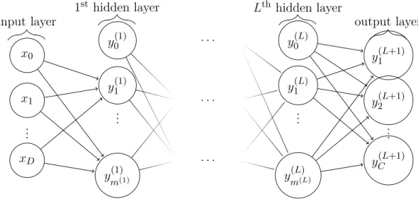
Definition 2.2.6. The Multi-Layer Perceptron (MLP) network uses several layers of these basic building blocks to form a recursive application of these functions:

p(y|x; ◊) = ‡(◊L‡(◊L≠1. . . ‡(◊0x))) (2.11)

In Figure 2.8 we can see a graphical depiction of the MLP.

For a regression problem, the last activation function is usually just a linear identity, while for classification problem, the last layer is usually a softmax layer that squeezes the activations into a distribution over classes p(y|x; ◊).

The problem of learning these parameters is usually posed into a frequentist optimization framework where the maximum likelihood estimator is maximized, which for convenience is treated as a minimization problem by minimizing the negative of the log likelihood:

arg min ◊ n ÿ i=1 ≠ log p(y|xi; ◊) (2.12)

x0 x1 ... xD y₀(1) y₁(1) ... y_m(1)₍₁₎ . . . . . . . . . _y(L) 0 y₁(L) ... y_m(L)_(L) y(L+1)₁ y(L+1)₂ ... y(L+1)_C input layer 1

st _{hidden layer L}th _{hidden layer}

output layer

Figure 2.8 Network graph of a (L + 1)-layer perceptron with D input units and C output units. The lth _{hidden layer contains m}(l) _{hidden units. Source: David Stutz, BSD 3-Clause}

license.

to the amount of data and model complexity, therefore a mini-batch Stochastic Gradient Descent (SGD) is used to optimize the parameters using only a portion of the data at each time. SGD works by iteratively updating the parameters according to the Algorithm 2.2.1. Algorithm 2.2.1 The general gradient descent algorithm; different choices of the learning rate “ and the estimation technique for ÒL(◊) may lead to different implementations.

Input: initial weights ◊(0)_{, number of iterations T} Output: final weights ◊(T )

1. for t = 0 to T ≠ 1 2. estimate ÒL(◊(t)₎

3. compute ◊(t)_{= ≠ÒL(◊}(t)₎

4. select learning rate “ 5. w(t+1):= w(t)+ “ ◊(t)

6. return w(T )

For neural networks, the gradient ÒL(◊(t)_{) is computed using backpropagation as described} in the Algorithm 2.2.1.

2.2.5 Convolutional Neural Networks (CNN)

Convolutional Neural Networks [59], also known as CNNs, are a class of specialized models that achieved enormous success in many practical applications. CNNs were inspired by the

Algorithm 2.2.1 Error backpropagation algorithm for a layered neural network represented as computation graph.

(1) For a sample (xn, ynú), propagate the input xn through the network to compute the outputs

(vi1, . . . , vi_{|V |}) (in topological order).

(2) Compute the loss Ln:= L(vi_{|V |}, yún) and its gradient ˆ_Ln ˆvi_{|V |}

. (2.13)

(3) For each j = |V |, . . . , 1 compute

ˆLn ˆwj = ˆLn ˆvi_{|V |} |V | Ÿ k=j+1 ˆvik ˆvik≠1 ˆvij ˆwj . (2.14)

where wj refers to the weights in node ij.

by the biological mechanism that was unveiled by Hubel and Wiesel in the 1950s and 1960s where two basic visual cell types were identified in the brain: the simple cells that were fired by straight edges having particular orientations within their receptive field and complex cells that have larger receptive fields and are insensitive to the exact position of the edges in the field.

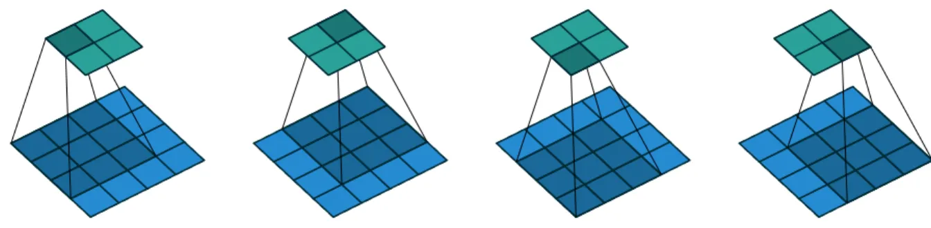
Figure 2.9 (No padding, unit strides) Convolving a 3 ◊ 3 kernel over a 4 ◊ 4 input using unit strides (i.e., i = 4, k = 3, s = 1 and p = 0). Source: Vincent Dumoulin et al. [4], MIT license. The main difference between a CNN and a vanilla MLP is that the CNN uses shared weights due to the convolutional component that uses a sliding window to apply the same weights, as seen in Figures 2.9 and 2.11. Another difference is the introduction of pooling layers that can be seen in Figure 2.12, that acts as a subsampling mechanism that can yield certain levels of rotation invariance to the network, although recently architectures can work well without pooling as well, especially for segmentation tasks, that will be discussed in the next section. In Figure 2.10 we show the architecture of a traditional CNN with convolutional layers followed

by non-linearities and subsampling layers. At the end of the CNN there is a fully-connected network, however, this fully-connected layer at the end isn’t that common anymore on modern architectures such as ResNets [55], that employ a global average pooling before the softmax activation. input image layer l = 0 convolutional layer with non-linearities layer l = 1 subsampling layer layer l = 3 convolutional layer with non-linearities layer l = 4 subsampling layer layer l = 6

fully connected layer layer l = 7

fully connected layer output layer l = 8 Figure 2.10 The architecture of the original convolutional neural network, as introduced by LeCun et al. (1989), alternates between convolutional layers including hyperbolic tangent non-linearities and subsampling layers. The feature maps of the final subsampling layer are then fed into the actual classifier consisting of an arbitrary number of fully connected layers. The output layer usually uses softmax activation functions. Source: David Stutz, BSD

3-Clause license.

input image

or input feature map output feature maps

Figure 2.11 Illustration of a single convolutional layer. If layer l is a convolutional layer, the input image (if l = 1) or a feature map of the previous layer is convolved by different filters to yield the output feature maps of layer l. Source: David Stutz, BSD 3-Clause license.

feature maps

layer (l ≠ 1) feature mapslayer l

Figure 2.12 Illustration of a pooling and subsampling layer. If layer l is a pooling and subsampling layer and given m(l≠1)₁ = 4 feature maps of the previous layer, all feature maps are pooled and subsampled individually. Each unit in one of the m(l)₁ = 4 output feature maps represents the average or the maximum within a fixed window of the corresponding feature map in layer (l ≠ 1). Source: David Stutz, BSD 3-Clause license.

2.2.6 Convolutional Neural Networks for Semantic Segmentation

Several works [60–62] applied convolutional neural networks for semantic segmentation, also called dense prediction. In dense prediction, the network usually outputs a prediction map with the same size of the input of the network with a prediction per each pixel of this output map.

Majority of the literature in the past were constrained by small models, patch-wise training due to the memory limitations, post-processing with superpixels, to name a few. One of the most important works that recently spawned a series of important developments for semantic segmentation is the work by [63] called Fully Convolutional Network (FCN), where the authors demonstrated that a fully-convolutional architecture trained end-to-end exceeded the state-of-the-art results when compared to its predecessors.

The main insight of the FCN was to combine coarse high layer information with fine, low layer information before up-sampling and producing the final predictions. The coarse features, coming from high layers contains semantic information that are merged together (simple summation) with the low layer features that contained the local information related to the fine spatial grid. By repurposing pre-trained networks into FCNs, the authors were also able to do transfer learning from networks trained on classification tasks such as ImageNet to semantic segmentation tasks.

After FCNs [63], a significant amount of follow-up works were developed. In medical imaging, one of the most prominent models that were developed based on the insights from FCNs is

the U-Net [64], where two different paths are combined with skip-connections to concatenate the feature maps. The first part is a downsampling path that uses traditional convolutional and pooling layers and the upsampling part where ‘up’-convolutions are used to increase the image size, creating an architectural shape of a U, hence the “U-Net” name.

In the Table 2.2 we show a summary of the currently available methods for the segmentation of the spinal cord gray matter. These methods are later expanded and described in the Chapter 4.

Table 2.2 Summary of the available methods for spinal cord gray matter segmentation. These are the methods that participated into the SCGM Challenge, it doesn’t cover all previously developed methods.

Method nane Year Initialization Training External data Time p /slice Summary

JCSCS [7] 2016 Auto. No Yes 4-5 min Uses OPAL [12] to detect the spinal cord and then STEPS to

do segmentation propagation and consensus segmentation using best-deformed templates.

DEEPSEG [16] 2017 Auto. Yes (4h) No <1 s U-Net with pre-trained weights using a restricted Boltzmann Ma-chine, uses a weighted loss function with two terms to balance sensitivity and specificity. Uses two models, one for cord segmenta-tion and another for GM segmentasegmenta-tion.

MGAC [15] 2017 Auto. No No 1 s Uses external tool "Jim" (from Xinapse Systems) to provide a initial guess for an active contour algorithm.

GSBME [2] 2017 Manual Yes (<1m) No 5 - 80 s Semi-automatic method that uses Propseg for cord segmentation with manual initialization followed by thresholding and outlier de-tection with image moments.

SCT [11] 2017 Auto. No Yes 8 - 10 s Atlas-based approach using a dictionary of manually segmented

WM/GM volumes projected into a PCA space, segmentation is done fusing labels.

VBEM [10] 2016 Auto. No No 5 s Semi-supervised, model intensities as a Gaussian Mixture trained

CHAPTER 3 OVERALL METHODOLOGY

This article based thesis is organized in the following section with the articles described below: • Article 1: Perone, C. S., Calabrese, E., & Cohen-Adad, J. (2018). Spinal cord gray matter segmentation using deep dilated convolutions. Nature Scientific Reports, 8(1). https://doi.org/10.1038/s41598-018-24304-3

• Article 2: Perone, C. S., & Cohen-Adad, J. (2018). Deep semi-supervised segmentation with weight-averaged consistency targets. DLMIA MICCAI, 1–8.

https://doi.org/10.1007/978-3-030-00889-5

• Article 3: Perone, C. S., Ballester, P., Barros, R. C., & Cohen-Adad, J. (2018). Unsupervised domain adaptation for medical imaging segmentation with self-ensembling. Submitted to Elsevier NeuroImage, under review. Short version presented at NIPS 2018 in the Medical Imaging Workshop.

In Chapter 4 we present the Article 1 where it is shown the design a Deep Learning methods for fully-automated segmentation of the spinal cord gray matter tissue from MRI volumes. In Chapter 5 we present the Article 2 where a semi-supervised learning method is developed to attack the problem of the low data regime present in medical imaging and finally in Chapter 6 we show the Article 3 where a unsupervised domain adaptation technique was developed for segmentation tasks in order to address the problem of poor generalization due to the distributional shift from different domains.

The main research questions we answer with present articles are the following:

• 1. How can deep learning methods improve on the current state-of-the-art results for segmentation of the spinal cord gray matter tissue ?

• 2. How can these segmentation methods be extended to take leverage of unlabeled data as well ?

• 3. How can we mitigate the generalization gap when applying these models to realistic scenarios where we have only unlabeled data from a new, different and unseen domain ?