SYSTEMATIC PARAMETER OPTIMIZATION AND APPLICATION OF AUTOMATED TRACKING IN PEDESTRIAN-DOMINANT SITUATIONS
DARIUSH ETTEHADIEH
DÉPARTEMENT DES GÉNIES CIVIL, GÉOLOGIQUE ET DES MINES ÉCOLE POLYTECHNIQUE DE MONTRÉAL
MÉMOIRE PRÉSENTÉ EN VUE DE L’OBTENTION DU DIPLÔME DE MAÎTRISE ÈS SCIENCES APPLIQUÉES
(GÉNIE CIVIL) DÉCEMBRE 2014
c
ÉCOLE POLYTECHNIQUE DE MONTRÉAL
Ce mémoire intitulé :
SYSTEMATIC PARAMETER OPTIMIZATION AND APPLICATION OF AUTOMATED TRACKING IN PEDESTRIAN-DOMINANT SITUATIONS
présenté par : ETTEHADIEH Dariush
en vue de l’obtention du diplôme de : Maîtrise ès sciences appliquées a été dûment accepté par le jury d’examen constitué de :
M. BILODEAU Guillaume-Alexandre, Ph. D., président
M. SAUNIER Nicolas, Ph. D., membre et directeur de recherche M. FAROOQ Bilal, Ph. D., membre et codirecteur de recherche M. MIRANDA-MORENO Luis F., Ph. D., membre
RÉSUMÉ
Les mouvements des piétons et leur modélisation constituent un domaine de recherche de plus en plus actif. Bien qu’encore souvent appliqué à la sécurité par l’élaboration de plans d’évacuation en cas d’urgence, comprendre le mouvement des piétons est un enjeu écono-mique de plus en plus important, notamment pour améliorer l’efficacité des aménagements de transport et des grands centres commerciaux.
Cependant, les données existantes — particulièrement au niveau individuel, ou microscopique — sont majoritairement collectées dans des situations expérimentales contrôlées. Elles ne sont donc pas nécessairement représentatives du comportement des piétons dans des situations réelles, particulièrement en tenant compte de la susceptibilité de leur comportement aux facteurs démographiques, psychologiques et environnementaux. Cette lacune est due princi-palement à l’absence de méthodes prouvées pour la détection et le suivi de piétons dans des cas réels, absence qui résulte de la complexité des mouvements piétons et qui persiste malgré l’avancement continu des méthodes automatique d’analyse.
De ces méthodes, la plus prometteuse est peut-être la détection et le suivi automatisé de piétons à partir de données vidéo. De tels outils ont non seulement démontré une capacité de suivi excellente (une précision atteignant 85 % dans certain cas), mais permettent aussi d’analyser des données vidéo enregistrées par les caméras de surveillance déjà installées. De tels résultats sont toutefois assujettis à deux limitations importantes, présentes dans la vaste majorité de la littérature. Premièrement, ces outils sont généralement testés sur une seule scène de mouvements piétons, ou sinon sur des scènes très similaires. Leur capacité à reproduire les performances publiées lorsqu’appliqués à une plus grande variété de cas est ainsi difficile à vérifier. Ceci est problématique car de nombreux problèmes affectent la performance des outils d’analyse vidéo et ces problèmes peuvent varier de manière importante entre scènes. Notamment, un piéton change de forme de manière continue lors de son mouvement, peut facilement être partiellement ou entièrement caché par un obstacle ou d’autres individus, et — contrairement aux véhicules routiers — n’est sujet à aucune contrainte concernant son trajet ou sa vitesse en dehors des obstacles physiques de son environnement.
La seconde limitation notée de ces outils est la manière dont ils sont calibrés. En effet, bien que la conception et la fusion de méthodes de détection sont communes, les paramètres sous-jacents semblent être le plus souvent choisis manuellement. De plus, avec une seule exception, ils n’ont jamais explicitement été le sujet d’optimisation rigoureuse. Il est ainsi probable que la performance optimale de ces outils n’a pas encore été révélée.
L’objectif du travail réalisé ici est donc la conception d’un algorithme générique d’optimisa-tion des outils de suivi de piétons. Acceptant comme entrée des trajectoires extraites manuel-lement d’une courte séquence vidéo (vérité terrain) et les paramètres de l’outil à optimiser, cet algorithme (nommée TrOPed, ou Tracker Optimizer for Pedestrians) produit des para-mètres calibrés pour produire les trajectoires les plus proches de la vérité terrain pour une scène particulière.
TrOPed est composé de trois fonctions principales. Au coeur est l’algorithme d’optimisation du recuit simulé (simulated annealing). Sélectionné pour son efficacité d’optimisation dans un domaine de recherche a priori inconnu (un facteur important vu la généralité désirée de l’algorithme ainsi que le temps important nécessaire à l’obtention de trajectoires dans la majorité des outils de suivi), cet algorithme régit de manière probabiliste le choix des paramètres de l’outil d’optimisation. Comme il permet le recul vers une solution inférieure, le recuit simulé peut s’échapper aux optima locaux et peut ainsi mieux localiser l’optimum global recherché.
Les paramètres sont déterminés à chaque itération par la seconde fonction, celle de mutation stochastique. Utilisant initialement des paramètres définis par l’utilisateur en fonction de leur distribution attendue, cette fonction réduit graduellement l’amplitude des ajustements des paramètres selon l’avancement de l’algorithme afin d’accélérer la convergence tout en assurant une solution finale précise.
La performance de chaque itération est évaluée par la troisième fonction, utilisant les mé-triques CLEAR MOT : MOTA (Multiple Object Tracking Accuracy, mesurant l’exactitude des trajectoires produites en fonction du nombre de piétons non détectés, de surdétections et d’associations fautives, avec une valeur optimale de 1) et MOTP (Multiple Object Tra-cking Precision, l’erreur spatiale moyenne, en mètres). Ces deux mesures sont combinées en une seule selon leurs poids relatifs, définis par l’utilisateur. Toutefois, les essais effectués ont démontré que les solutions optimales sont atteintes en utilisant MOTA uniquement.
Finalement, TrOPed inclut des mécanismes et paramètres additionnels, optimisés en parallèle à ceux de l’outil calibré, qui permettent d’optimiser la méthode typique de projection des trajectoires de l’espace image des vidéos vers les coordonnées réelles. Cette transformation est communément effectuée vers des coordonnées définies au niveau du sol, ce qui est peu problématique lors d’enregistrement fait à longue distance ou de véhicules. Cependant, dans le cas de piétons (qui sont notamment plus grands que larges) et la proximité typique des caméras utilisées pour les enregistrer, la différence entre le plan du sol et le plan parallèle dans lequel les piétons sont détectés devient une source importante d’erreur. Des paramètres régissant l’élévation de ce second plan ont donc été inclus.
Les essais de TrOPed ont été effectués sur deux outils de suivis : Traffic Intelligence (TI) etUrban Tracker (UT). Ces deux outils utilisent des méthodes différentes de détection, per-mettant de vérifier la généralisabilité de l’algorithme : TI identifie le mouvement de groupes de pixels et les regroupe en piétons, et UT distingue les "blobs" de mouvement par comparaison avec l’arrière-plan statique.
Afin de traiter différents niveaux de complexité, trois scènes ont été étudiées : un corridor central à l’université Polytechnique Montréal, l’entrée d’une station de métro, également à Montréal, et un passage piéton au centre-ville de la ville de New York localisé en face de la station de train centrale. Les deux premiers cas ont été enregistrés pendant l’heure de pointe matinale, avec des caméras installées à un angle et une distance approximant ceux typiques des caméras de surveillance. Le troisième cas, quant à lui, a été enregistré entre 10h et 13h un jour de semaine, et la caméra installée verticalement directement au dessus du passage. Pour toutes les scènes, deux séquences de une minute chacune — choisies pour leur représentativité des scènes en général — ont été extraites et les trajectoires des piétons individuels extraites manuellement. De ces séquences, l’une a servi à la calibration par TrOPed, et la seconde à vérifier si les paramètres calibrés étaient adaptés aux scènes en entier ou étaient trop optimisés pour la première séquence (suroptimisation).
Dans tous les cas, les paramètres optimisés par TrOPed ont produit des trajectoires d’exac-titude et de précision supérieures à celles obtenues par calibration manuelle des outils ; en moyenne, cette amélioration s’est traduite par une réduction de 50 % (+/- 15 %) des erreurs commises. Cette amélioration s’est maintenue lors des essais sur les séquences tests, malgré une légère baisse de performance attribuable à la suroptimisation. L’amélioration a aussi été maintenue peu importe les paramètres initiaux, confirmant que la solution finale représente très probablement un optimum global.
Lors des initialisations sur des paramètres choisis arbitrairement, ces résultats ont été obtenus après une centaine d’itérations pour UT, et approximativement 2000 pour TI, une différence attribuable au plus grand nombre de paramètres et une plus grande gamme de valeurs pour ces paramètres. Cependant, comme TI produit des trajectoires près de 50 fois plus rapidement que UT, dans les deux cas la procédure a été complétée en moins de 24 heures.
Des essais comparant l’optimisation avec et sans les paramètres affectant l’homographie ont montré que, comme attendu, la modification de l’élévation du plan de projection permet d’améliorer la précision des trajectoires. De plus, lorsqu’appliqué à TI (qui utilise les co-ordonnées projetées au cours du suivi des piétons), ces paramètres ont aussi permis une amélioration de MOTA d’entre 5 et 20 % selon la scène.
TrO-Ped sur l’entièreté des données vidéos ont été visualisées et analysées. Les cartes de densités relatives ainsi produites confirment que ces trajectoires représentent adéquatement le compor-tement piéton de chaque scène. De manière semblable, l’analyse des distributions de vitesses est en accord avec la littérature et avec les phénomènes observés, et les comptages direction-nels automatisés — bien qu’erronés sur le même ordre de grandeur que les trajectoires — demeurent représentatifs des volumes relatifs réels.
La limitation principale de ces travaux est l’utilisation de seulement deux outils de suivis, qui n’ont pas été conçus spécifiquement pour le suivi de piétons. Ainsi, bien que les résultats obtenus démontrent une amélioration importante sur la calibration manuelle, la performance demeure inférieure ou égale à ce qui a été publié dans la littérature sur le suivi des piétons. Des travaux futurs devraient donc se concentrer sur l’essai de TrOPed sur des outils plus spécialisés, ce qui permettrait de vérifier si les améliorations obtenues ici se généralisent. Si tel est le cas, et des MOTA de 0.90 ou plus peuvent être régulièrement atteints, la collecte de données automatisées sur les piétons dépasserait enfin la performance de la collecte manuelle à un cout nettement moins élevé.
ABSTRACT
Though a wealth of data exists for the characterization of pedestrian movement, a majority of it originates from experimental settings owing to the current state of trackers for real-world scenarios. While these trackers are steadily improving, they remain insufficiently reliable for the accurate, microscopic tracking of individuals, particularly in cases of occlusion or higher density, complex scenes. In this work, the use of evolution algorithms is proposed for the systematic calibration of the parameters of existing trackers in order to further optimize their performance – evaluated by tracking accuracy and precision metrics – in complex cases, with an initial focus on two tracking methods designed for multimodal analysis. This calibration is further aided by the inclusion of additional parameters regulating homography, or specifically the plane to which tracker detections are projected. Three real test cases were used: a) a confined corridor in a public building, b) a subway station entrance during morning rush hour and c) a crosswalk in downtown New York. Results demonstrate a halving of tracking errors over both default and manually-calibrated parameters, as well as a strong correlation in performance between similar cases. These results were consistent over multiple trials and regardless of the starting parameters, strongly implying that the obtained solutions are indeed the global maxima for each scene. For application and validation of the resultant tracks, flow characterization and directional counting are demonstrated, utilizing tools included in the optimization framework.
TABLE OF CONTENTS
RÉSUMÉ . . . iii
ABSTRACT . . . vii
TABLE OF CONTENTS . . . viii
LIST OF TABLES . . . xi
LIST OF FIGURES . . . xiii
LIST OF ABBREVIATIONS . . . xviii
LIST OF APPENDICES . . . xix
CHAPTER 1 INTRODUCTION . . . 1
1.1 Context . . . 2
1.2 Problem Statement . . . 3
1.2.1 Complexity of Pedestrian Movement . . . 3
1.2.2 Evaluating Extracted Data . . . 4
1.2.3 Optimization Methodology . . . 5
1.2.4 Extracting Meaningful Data . . . 5
1.3 Objectives . . . 6
1.4 Document Structure . . . 7
CHAPTER 2 LITERATURE REVIEW . . . 9
2.1 Pedestrian Models . . . 9
2.1.1 Gas particle model . . . 10
2.1.2 Fluid dynamics model . . . 11
2.1.3 Cellular automata . . . 12
2.1.4 Mesoscopic models . . . 13
2.1.5 Discrete choice models . . . 14
2.1.6 Social force model . . . 15
2.2 Data collection methods . . . 17
2.2.1 Point and line data-collection methods . . . 17
2.2.3 Video-based methods applicable to real-world cases . . . 21
2.2.4 Trackers Used in this Work . . . 29
2.3 Video-tracking metrics . . . 31
2.3.1 The VACE metrics . . . 34
2.3.2 The CLEAR MOT metrics . . . 36
2.3.3 Associating Detected with Ground-Truth Objects . . . 37
2.4 Optimization methodologies . . . 37 CHAPTER 3 METHODOLOGY . . . 43 3.1 Optimization Schema . . . 43 3.2 Data-Collection . . . 44 3.2.1 Data-Collection Method . . . 45 3.2.2 Test Cases . . . 46
3.3 Establishing the Ground-Truth . . . 49
3.3.1 Sequence selection . . . 49
3.3.2 Ground-Truth Annotation . . . 49
3.4 Algorithm Inputs . . . 51
3.5 Homography Parameters . . . 53
3.6 Metric Selection and Performance Evaluation . . . 57
3.6.1 Metric Selection . . . 57
3.7 Optimization Algorithm . . . 60
3.8 State-Generation Function . . . 61
3.9 Final Algorithm . . . 63
3.10 Calibration, or : the tragic irony of building a parameter optimization algo-rithm that itself has twelve parameters . . . 64
3.10.1 Complete Algorithm Diagram . . . 68
CHAPTER 4 OPTIMIZATION RESULTS . . . 69
4.1 Overall Results . . . 69
4.2 Observed Algorithm Behavior . . . 74
4.2.1 Sensitivity to Starting Parameters . . . 76
4.3 Tracker Performance . . . 77
4.3.1 Homography Parameters . . . 77
4.3.2 Traffic Intelligence . . . 81
4.3.3 Urban Tracker . . . 83
4.4 Sensitivity to Test Cases . . . 85
4.4.2 Subway Station . . . 86
4.4.3 New York Crosswalk . . . 87
CHAPTER 5 APPLICATION AND DISCUSSION . . . 90
5.1 Applications of the Optimized Trackers . . . 90
5.1.1 Tracks . . . 90
5.1.2 Density Maps . . . 94
5.1.3 Speed Profiles . . . 97
5.1.4 Directional Counts . . . 99
5.2 Revised Clear MOT Metrics . . . 101
5.3 Discussion . . . 103
CHAPTER 6 CONCLUSION . . . 106
6.1 Summary . . . 106
6.2 Limitations and Future Work . . . 107
REFERENCES . . . 109
LIST OF TABLES
Table 2.1 Summary of selected pedestrian tracking methods. It should be noted that reported accuracies were evaluated in different scenes and with a variety of metrics, making direct comparison difficult. Pedestrian den-sities reported in the table correspond to a visual evaluation of density in the scenes : low density denotes that individuals are generally clearly separated, while high density implies substantial occlusion and/or grou-ping of pedestrians. DR : Detection Rate, calculated differently for each author. Source : Ettehadieh et al. (2014). . . . 30 Table 2.2 List of Traffic Intelligence parameters affecting detection and tracking,
along with their range and description. . . 41 Table 2.3 List of Urban Tracker parameters affected detection, tracking and
post-processing of trajectories, along with their range and description. . . 42 Table 3.1 Macroscopic characterization of the test and calibration sequences.
"Atypical" objects refer to those not moving in the bidirectional axis of highest flow in the sequence. . . 51 Table 3.2 Parameter update equations for variable X between iterations i and
i+1 in the three operations currently included in TrOPed and defined in the variable parameters file. The above equations are for floating-point variables ; other data types use slightly modified versions. . . . 52 Table 3.3 Structure of the input file for tracker parameters to be optimized. . . 53 Table 3.4 Variable parameters selected for optimization by TI and UT, as input
into TrOPed. prev indicates a parameter dependent on the previous one to define either its maximum or minimum value. . . 56 Table 3.5 MOTA as evaluated by TrOPed and Jodoin et al. (2014) for both
studied trackers. Scene, tracker parameters, matching distance and ground-truth were provided from the latter authors for testing. . . 60 Table 3.6 Algorithm parameter values after manual calibration. . . 66 Table 4.1 MOTA and MOTP performance of Traffic Intelligence before and after
optimization, as well as for manually calibrated parameters. MOTP is presented according to the standard definition (average error in meters) rather than the normalized version utilized by TrOPed. . . 70
Table 4.2 MOTA and MOTP performance of Urban Tracker before and after op-timization, as well as for manually calibrated parameters. The absence of MOTP results in two subway station tests indicates that the tra-cker failed to produce sufficient meaningful tracks. As above, MOTP is presented according to the standard definition (average error in meters). 70 Table 4.3 Convergence times of TrOPed for the test cases, both to best solution
and to cessation of the algorithm. Times in hours are approximate. . 74 Table 4.4 Detailed performance of Traffic Intelligence on the three test cases.
Percentages represent the ratio of the related error to the number of ground-truth tracks, which is equivalent to the absolute MOTA reduc-tion caused. . . 82 Table 4.5 Detailed performance of Urban Tracker on the two functioning test
cases. Percentages represent the ratio of the related error to the num-ber of ground-truth tracks, which is equivalent to the absolute MOTA reduction caused. . . 84 Table 5.1 Comparison of performance and error rates after optimization of TI
LIST OF FIGURES
Figure 1.1 Examples of interpretable and misleading errors for near-identical accu-racy and precision, as measured by the CLEAR MOT metrics described in section 2.3.2. Each circle represents the detection of an object in a single frame. . . 7 Figure 2.1 Different levels in pedestrian walking behavior. Source : Sahaleh et al.
(2012). . . 10 Figure 2.2 A pedestrian, its possible directions of motion, and corresponding
pro-babilities for the case of a von Neumann neighborhood. Source : Sahaleh et al. (2012). . . . 12 Figure 2.3 Example network used in early mesoscopic models. Inspired by Hanisch
et al. (2003). . . . 13 Figure 2.4 Discretization of space based on 3 speed regimes and 7 radial directions.
Inspired by Antonini et al. (2004). . . . 15 Figure 2.5 Example of a macroscopic pedestrian study, with data collected
ma-nually from recorded footage. The time each of the two screenlines (the red vertical lines) is crossed by a pedestrian is recorded manually, al-lowing both velocity and density measurement. Source : Seyfried et al. (2005b). . . 17 Figure 2.6 Microscopic video tracking using colored uniforms as visual cues. Source :
Hoogendoorn et al. (2003a). . . . 19 Figure 2.7 Real-world pedestrian tracking, using specially-installed overhead
ca-meras and a close angle. Source : Johansson et al. (2007a). . . . 20 Figure 2.8 Illustration of the processing of an example frame used in the tracking
of pilgrims near Makkah, Saudi-Arabia, from the original image (top left) to the resultant detections (bottom right). Source : Johansson and Helbing (2008). . . 21 Figure 2.9 Example of feature detection and subsequent (mostly erroneous)
grou-ping, as performed by Traffic Intelligence before optimization. . . 23 Figure 2.10 The four phases of background subtraction. From left to right : video
frame, background model, foreground detection, and final foreground after segmentation and cleaning. Source : Jodoin et al. (2014). . . . . 25
Figure 2.11 Application of default (a to c) and evolutionarily optimized (d to f) background subtraction to single pedestrian tracking. Source : Pérez et al. (2006b). . . . 26 Figure 2.12 Visual cues used in HOG-based detection to generate target outlines.
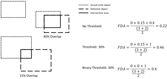
In each triplet is displayed, from left to right : (1) the input image, (2) the corresponding HOG feature vector (the dominant orientation in each cell), (3) the dominant orientations after post-processing by Support Vector Machines. Source : Dalal (2009). . . 28 Figure 2.13 Illustration of the typical errors commited by automated trackers. . . 33 Figure 2.14 Sample example demonstrating the calculation of FDA with various
thresholds. Inspired by Kasturi et al. (2009) . . . . 35 Figure 3.1 Flow diagram of the TrOPed algorithm. Source : Ettehadieh et al. (2014). 43 Figure 3.2 Lens distortion in the New York video sequence (left) and the same
frame after correction by the tool included with Traffic Intelligence (right). Note that though these frames are presented at the same size for clarity, the left one is 1920x1080 pixels, whereas that after correction is 2515x1415 pixels. . . 46 Figure 3.3 Example frames taken from the two recording locations. (a) and (b)
represent the two camera angles used in the Polytechnique corridor, (c) and (d) from the sole camera used for optimization at the subway station, with the former showing minimum pedestrian density and the later taken during the arrival of a bus. . . 47 Figure 3.4 Presentation of the annotation tool used to manually extract
ground-truth trajectories : pedestrians are located by their bounding boxes, and identified by number according to the order in which they were tracked. . . 50 Figure 3.5 Illustration of the effects of low recording angles (b) the height of
pe-destrians (c) and both (d) on positional tracking error, relative to the common case of vehicle tracking in (a). (e) presents the proposed so-lution : optimization of the elevation of the homography plane to cor-respond with the elevation at which pedestrians are most commonly detected. . . 54 Figure 3.6 Schematic representation of the added homography-elevation
parame-ters and their effect. Note that the elevations are not necessarily equal for each hi. . . 55
Figure 3.7 Example visualization of mid-optimization tracks in the Polytechnique corridor sequence. . . 63 Figure 3.8 Example frame from the Polytechnique atrium sequence, used for
cali-bration of TrOPed. . . 66 Figure 3.9 MOTA improvements during optimization with TrOPed on the atrium
sequence, for both the first set of functioning parameters (i.e. those converging to a solution) and after manual calibration. In both cases, initial tracker parameters were set as far from the known optimum as possible (i.e. either their maximum or minimum values) so as to maximize convergence time. . . 67 Figure 3.10 Complete flow diagram of TrOPed. . . 68 Figure 4.1 Comparison of manual and optimized parameter performance using
Urban Tracker. Negative values are not fully displayed, and crashes on the New York sequences precluded performance evaluation. . . 71 Figure 4.2 Comparison of manual and optimized parameter performance using
Traffic Intelligence. Note that large negative values are not fully displayed. 71 Figure 4.3 MOTA scores for Traffic Intelligence parameters on the calibration and
test sequences. . . 72 Figure 4.4 Relationship between MOTP and MOTA scores across all cases and
both trackers. . . 73 Figure 4.5 Evolution of last-best MOTA scores during optimization for the three
calibration sequences with Traffic Intelligence. . . 75 Figure 4.6 Evolution of last-best MOTA scores during optimization for the three
calibration sequences with Urban Tracker. Values below zero are not shown. . . 75 Figure 4.7 Evolution of MOTA scores during optimization of TI, initialized with
manually-calibrated parameters. . . 77 Figure 4.8 Optimized point-correspondence elevations. Point numbering in all cases
begins in the right-most foreground, and proceeds counter-clockwise. 78 Figure 4.9 Trajectories produced by optimized Traffic Intelligence in the
Poly-technique corridor calibration sequence, with and without optimized homography elevation. Lens distortion was not corrected for in this trial, leading to the exaggerated curvature of the tracks on the lower portion of the corridor. . . 79
Figure 4.10 Comparison of ground-truth and example tracks plotted every 10 frames for a single pedestrian in the New York sequence, using default (labelled manually calibrated) and optimized homography elevations. . . 80 Figure 4.11 Example frame of Traffic Intelligence tracking on the Polytechnique
calibration sequence. . . 82 Figure 4.12 Example of Traffic Intelligence failing to dissociate visually distinct
targets. . . 83 Figure 4.13 Representative frame of Urban Tracker on the Polytechnique
calibra-tion sequence. . . 85 Figure 4.14 Typical tracker failure in the subway station scene : pedestrians
ap-proaching from opposite the camera were often highly grouped together both in reality and by the trackers. . . 87 Figure 4.15 Example frame of TI tracking on the New York crosswalk sequence. . 88 Figure 5.1 Trajectories produced by optimized Traffic Intelligence for a 30 minute
sequence in the Polytechnique corridor scene. . . 90 Figure 5.2 Trajectories produced by optimized Traffic Intelligence for a 30 minute
sequence in the subway station scene. . . 91 Figure 5.3 Trajectories produced by optimized Traffic Intelligence for a 30 minute
sequence in the New York crosswalk scene. . . 92 Figure 5.4 New York crosswalk trajectories, filtered to only represent near-horizontal
(crossing) tracks. . . 93 Figure 5.5 New York crosswalk trajectories, filtered to only represent near-vertical
(vehicular and sidewalk) tracks. . . 93 Figure 5.6 Heatmap of pedestrian detection in the Polytechnique corridor
se-quence. Hexes are approximately 0.4 meters wide. Note that colors represent individual tracker detections, not pedestrians. . . 94 Figure 5.7 Heatmap of pedestrian detection in the subway station sequence. Hexes
are approximately 0.4 meters wide. . . 95 Figure 5.8 Heatmap of pedestrian detection in the New York crosswalk scene,
filtered to display only near-horizontal tracks. Hexes are approximately 0.4 meters wide. . . 96 Figure 5.9 Heatmap of pedestrian detection in the New York crosswalk scene,
filtered to display only near-vertical tracks. Hexes are approximately 0.4 meters wide. . . 96 Figure 5.10 Speed distribution for the Polytechnique corridor video. . . 97 Figure 5.11 Speed distribution for the subway station video. . . 98
Figure 5.12 Speed distribution for the New York crosswalk video. . . 98 Figure 5.13 Counting thresholds (left) and comparison of automated vs. manual
counts (right) for the Polytechnique corridor video. . . 100 Figure 5.14 Counting thresholds (left) and comparison of automated vs. manual
counts (right) for the subway station video. . . 100 Figure 5.15 Counting thresholds (left) and comparison of automated vs. manual
LIST OF ABBREVIATIONS
TrOPed Tracker Optimizer for Pedestrians MOTA Multiple Object Tracking Accuracy MOTP Multiple Object Tracking Precision TI Traffic Intelligence
LIST OF APPENDICES
CHAPTER 1 INTRODUCTION
Walking is both the most ancient and the most ubiquitous of transit modes. All trips at the very least begin and end with pedestrian locomotion, and inter- (as well as intra-) modal transfers necessarily implicate additional pedestrian phases when they take place. Conse-quently, high-density areas - and transit hubs in particular - benefit greatly from designs emphasizing pedestrian movement, both in their role as feeder systems for other modes and to ensure adequate evacuation in the case of an emergency. More broadly, such designs may be applied to increase the attractiveness of walking as a larger part of commutes, and to both evaluate and maximize the profitability in the commercial sector ; indeed, the latter is a substantial and growing area of research, particularly in supermarkets (see Larson et al., 2005).
Optimizing spaces for pedestrian use requires the capacity to accurately and reliably model their behavior, and to predict their movement patterns in response to obstacles, events, distractions, each other, or in the absence of any such factors. Said capacity, in turn, must be built on a thorough understanding of pedestrian behavior in a variety of contexts.
Unfortunately, observing pedestrians’ movement in sufficient spatiotemporal resolution to build and calibrate the aforementioned models has proven to be a difficult problem : the most accurate methods for individual - or microscopic - tracking are currently inherently limited to experimental (or at best, very specific) settings. More generalizable methods, in contrast, demonstrate considerably more errors upon visual validation, though their performance has been steadily improving over the last decade.
In an effort to bridge this divide, this work presents a generalizable evolutionary algorithm for the calibration of video-based tracking methods in order to improve both their accuracy and precision, in essence revealing any untapped potential a tracker may possess. Such algorithms have been applied to pedestrian tracking once before : Pérez et al. (2006a) applied evolutio-nary optimization to a single stage of their tracker, attaining a 25% reduction in positional error. In contrast, instead of targeting specific facets of the problem, the method presented herein aims at optimization of the entire tracking method. While the focus here is on ex-tracting trajectories from video data, this method should be applicable to any microscopic trajectory-extraction method.
1.1 Context
The need for improved pedestrian models and design is steadily growing. While historically this has been the result of rapid urbanization since the industrial revolution (with simi-lar trends more recently in developing nations) the 21st century has seen the demand for pedestrian analysis compounded through the global favoring of higher capacity structures and municipal desires to consolidate urban populations around existing transit networks (for example, City of Montreal, 2002).
Of course, existing designs are not bereft of pedestrian modelling, including both macroscopic and microscopic models. The former are advantaged by the fact that data collection for macroscopic behavior (i.e. the movement of pedestrians at the level of corridors and/or other subdivisions of an area, as opposed to that of each individual) can be performed through established methods. These methods include crowd size estimates, counts (manual, by RFID or with turnstiles), infrared detectors, pressure pad sensors and origin-destination surveys. In contrast, microscopic models (at least, those that are not proprietary) lack proven data-collection methodologies, being validated through one of three methods :
– macroscopic data : while microscopic models should be capable of reproducing macro-scopic observations, using these as the sole means of both calibration and validation defeats the purpose of increased model resolution, making the influence of smaller design elements difficult to distinguish within the studied area as a whole.
– manually obtained data : establising pedestrian trajectories manually (habitually from video data, given that doing so on the scene is a very difficult task) is a reliable, accu-rate, but extremely time consuming process ; model validation with such data is therefore habitually performed with relatively small datasets (for example, Robin et al., 2009). – data from experimental settings : given the added control afforded to researchers in
the experimental setting, the extraction of accurate pedestrian trajectories using either of the above methods is greatly facilitated. However, whether the data gathered in these situations is truly representative of real cases is questionable.
A fourth potential validation method exists in microscopic data extracted from real cases. It has however yet to achieve widespread use, a fact which can likely be attributed to its current poor performance in comparison to the methods presented above. Of the potential microscopic methods, those based on typical video data (as opposed to infrared, thermal or binocular video) have several notable advantages. First, the required equipment is already in widespread use for other purposes (e.g. surveillance) ; this ubiquity means data for emergency or other particular situations can be made available. Second, where the equipment is not already in
place, its low cost and availability makes installation simple. Third and finally, the nature of the data makes visual validation relatively easy. The latter point is of particular importance in the method presented in the present work, yet all contribute to its generalizability.
1.2 Problem Statement
The primary problem addressed by this work is the need for increased performance in pe-destrian tracking, coupled with the current absence of explicit calibration of tracking tools. This problem can be subdivided into the four following difficulties :
1.2.1 Complexity of Pedestrian Movement
Over the last two decades, video tracking of road vehicles has made great strides ; though it cannot yet be considered a solved problem, vehicle trackers have demonstrated the capacity to generate trajectories with both robust accuracy and precision (see Mei and Ling, 2011, for example). However, while one might expect this progress to translate more or less seamlessly to pedestrian tracking due to the superficial similarity of the tasks, several characteristics of pedestrians and their movement render their tracking substantially more difficult.
First, pedestrians make up a particularly heterogeneous group. In contrast to road vehicles, for which vehicle attribute and driving behavior are regulated and enforced, there are no restrictions on who may be a pedestrian and they are, for the most part, free to travel at the speed and via the paths they desire. Their behavior is also subject to a larger number of influent factors. These include those equally influencing motorists, such as age (Himann et al., 1988) and alcohol use (Oxley et al., 2006), as well as additional attributes such as physical fitness (Schlicht et al., 2001) and trip purpose (Hoogendoorn and Bovy, 2004). One famous example perhaps best illustrating pedestrians’ sensitvity to outside factors is that of Bargh et al. (1996) : exposure to words stereotypically associated with age - for example prune instead of the the control word apple - was found to significantly slow walking speed immediately afterwards (though it should be noted that the true source of this effect has since been disputed). More obviously, there is the sensitive case of those with visual, physical, or other impairments. Though it would certainly be extremely impractical (and perhaps unnecessary) to include all such factors in a single model - particularely given that some, such as fitness, may be impossible to observe - ensuring their adequate representation in an experimental setting would be a substantial undertaking.
Second, pedestrian movement is far less restricted than that of vehicles. Vehicles are constrai-ned both to a small number of permitted paths at any given moment - as delimited by signals,
speed limits, lanes, and safe distance from other vehicles - and to a limited range of motion (notably, a stopped vehicle can begin moving only forwards or backwards). Pedestrians, ho-wever, are constrained primarily by their own physical ability and whatever obstacles may be in their path. They may also form groups and move together or interweave when crossing paths, exacerbating both the complexity of their movements and the third problem with their tracking.
Indeed, even if the two preceding factors could somehow be negated, human beings remain difficult targets to track. The safe distance maintained between vehicles, combined with their rigid bodies, both allows their apparent shapes to remain relatively constant and limits instances of occlusion. Both these factors greatly facilitate tracking, as they generally result in more isolated and consistent targets. Pedestrians, on the other hand, implicate their entire bodies in locomotion, changing shape with each stride or during any other action they take as they walk. They also occupy much more space vertically than in the horizontal plane within which their movement occurs. When combined with their greater propensity to move in close proximity to each other, this lends itself both to occlusion of those individuals farther from the camera and to greater difficulty distinguishing individuals within a group.
Fourth and finally, one must consider how the above issues are compounded by the hetero-geneity of pedestrian areas themselves. It is highly unlikely that pedestrian attributes in an office building are as varied as within a shopping mall, that their movement is as chaotic as in a secondary school, or that their flow is as dense as in a rush-hour transit hub. As a result, both the specific challenges and overall difficulty faced by a pedestrian tracker can vary wildly between cases ; performance in one case may not be particularly indicative of that in another.
1.2.2 Evaluating Extracted Data
Evaluating said performance is, in itself, problematic. No single, standardized metric exists (see section 2.3) making comparisons between trackers difficult, and yet some basis for com-parison is necessary for one to proffer a method as an improvement upon another.
Fundamentally, a video-based tracker must execute two tasks : it must detect and track the objects of interest, as well as locate them within the search space. Tracker performance therefore globally consists of two factors, accuracy and precision, each relating to one of these tasks. Accuracy refers to the ability to correctly detect targets within the observed space, and to maintain that detection as the target moves. Precision is a function of the error in the targets’ location, or how well the tracker locates the objects it detects. Both these measures must be adequate for the resulting tracks to be of use.
Unfortunately, within an optimization framework (such as that proposed here) evaluating performance via two inherently different dimensions is problematic, as the resulting perfor-mance measures are mathematically incomparable. Accuracy and precision must therefore somehow be fused into a single measure or, alternatively and if possible, optimization must take place for each one in sequence.
Each metric must also individually be calculated in a robust and consistent manner. What constitutes an accurate detection must be defined, and should exclude nonsensical track-object matching (e.g. associating the movement of branches in the wind to a passing pedes-trian) while not implicitly imposing excessive precision requirements by necessitating perfect matches. Both measures should be consistent with the subjects being tracked and the appli-cations being considered, particularly in regards to scale : given the low camera angles and small distances involved in much available pedestrian video data, the effect of perspective renders distances in the video-frame a poor substitute for those in the observed space.
1.2.3 Optimization Methodology
Improving performance as measured by the above metrics has been the subject of research for a number of years ; a brief overview of these efforts is presented in section 2.2. The primary approach, however, has been the development and fusion of novel methods and not the optimization of existing ones, for which calibration (though rarely reported) appears to be performed manually
This suggests that further optimization could be beneficial, but also signifies that the search space for many - if not all - trackers is largely unexplored. Said space is also usually broad and complex, as trackers have a tendency towards having a large number of parameters, many highly sensitive. The selected optimization method must therefore be rigorous. However, the only means by which to test a given set of parameters is through the tracker. The best performing of these run in real time (some an order of magnitude slower) and a test sequence must be sufficiently lengthy in order to be representative of the scene as a whole and so avoid overfitting of the tracker. The optimization method must therefore converge to a solution relatively rapidly lest the process take an inordinate amount of time.
1.2.4 Extracting Meaningful Data
One final consideration, related to that presented in 1.2.2, is that the trajectories output by the tracker must represent the ground-truth (or real trajectories of the pedestrians) in such a way as to be meaningful in subsequent analysis. This can, in part, be evaluated by accuracy
and precision - indeed, if both are perfect, the data is by definition perfectly representative. In the inevitable case that errors do occur, however, these metrics provide only a partial portrait of their gravity.
Figure 1.1 presents three simple examples : though the two rightmost columns are extremely similar in terms of estimated accuracy and precision, ground-truth in the center column can relatively easily be extrapolated either by human verification or simple heuristics in post-processing. In contrast, the tracks in the column on the right are ambiguous, poten-tially misleading. And yet, all the presented tracks would perform on par with the leading contemporary metrics, with accuracies ranging between 80 and 90 percent according to most metrics.
This behavior is troublesome, especially during optimization, as the parameter sets leading to two such ostensibly similar solutions are unlikely to be similar themselves, but instead may represent distinct local maxima - a phenomenon equally likely to present itself, albeit more discretely, at the lower performances encountered early in the optimization process.
1.3 Objectives
The objective of this project is the development of an optimization framework for the im-provement of video-based pedestrian tracker performance. More specifically, the approach described herein targets the oft-ignored calibration of tracking tools, particularly in regards to optimization for specific scenes. Said framework aimed to fulfill the following criteria : – Significant improvement over existing calibration methods : The optimization
can only be deemed successful if it attains marked improvement over previous tracker calibration methods (manual calibration, for the trackers examined herein).
– Minimal dependence on starting parameter values : In order to both maximize au-tomation and ensure the provided solutions represent global maxima, optimization should be independent of the input tracker parameters.
– Efficient convergence time : Given the problems stated in 1.2.3, it is likely that many optimization algorithms result in convergence times best measured in weeks or months -comparable to what would be required to simply extract the data manually, though of course this would be much more time-consuming for the researcher. Minimizing run-time should therefore be a priority.
– Generalizability : The framework should be applicable to a large number of different trackers, regardless of their methodologies or characteristics. Said trackers are not limited to pedestrians ; indeed, while pedestrians present a unique combination of tracking difficulties,
Ground-Truth Interpretable Errors Misleading Errors
Figure 1.1 Examples of interpretable and misleading errors for near-identical accuracy and precision, as measured by the CLEAR MOT metrics described in section 2.3.2. Each circle represents the detection of an object in a single frame.
tracking methods are nearly universal regardless of the target objects. Furthermore, as all video analysis is to be performed by the optimized tracker, the method presented herein is also not limited to video tracking, but to all automated tracking applications.
1.4 Document Structure
The present document consists of seven sections. The present section, the introduction, serves to present the overall subject matter, as well as the primary research objectives and expected obstacles. The literature review follows, summarizing both the state of the art in pedestrian tracking and modelling, as well as other research topics pertaining to the present subject. The third section presents the fundamental methodology of the developed software, both as it functions as a whole as well as the individual underlying processes. The document continues
with the presentation of the results of optimization with the constructed tool in section five, followed by examples of the extracted data and their comparability to data extant in the literature in a sixth section. It concludes with a general overview of the results, as well as discussion of the observed limitations of the project and potential avenues for future work.
CHAPTER 2 LITERATURE REVIEW
This section presents an overview of the state of the art of pedestrian models and data-gathering methods, as well as potential optimization algorithms and video-tracking metrics.
2.1 Pedestrian Models
Pedestrian models serve to represent and predict walking behavior as it occurs in reality. They achieve this by simplifying said behavior into a set of mathematical heuristics, which are subsequently calibrated using available real-world or experimental data. Pedestrian modelling is generally performed on one of three scales (Sahaleh et al., 2012) :
– microscopic or disaggregate models : Also sometimes refered to as agent-based mo-dels. At this scale, each pedestrian is simulated individually, with the movements and actions estimated independently of other agents. Every individual’s position is established according to a preselected unit-time while they are in the simulated area.
– macroscopic or aggregate models : Analysis of pedestrians as groups, with individuals existing only as members of an aggregate. System state is generally described by the density, flow and average velocity of groups ; individuals are not distinguishable from each other. As such, these models are particularely reliant on accurate fundamental diagrams, which define velocity as a function of density (Schadschneider et al., 2009).
– mesoscopic models : A compromise between the previous two scales, mesoscopic models simulate pedestrians in aggregate terms. They can, however, render a microscopic portrait of an area, albeit probabilistically (Teknomo and Gerilla, 2008).
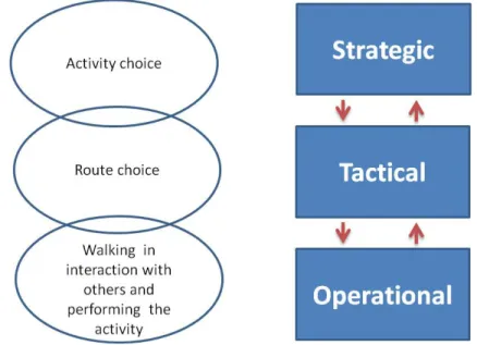
Regardless of scale, a complete theory of pedestrian dynamics usually takes into account three levels of behavior (defined in Hoogendoorn et al., 2002) :
– Strategic level : At the highest level, pedestrians decide what activities to perform, as well as where and when, with no knowledge of the network or potential routes. This information resembles (and is possibly best represented by) origin-destination surveys. Indeed, within a given simulation, this data serves as an input parameter, and tends to be either observed in or extracted from such surveys before being utilized in the following stage.
– Tactical level : At the tactical level, individuals take the network into consideration so as to decide upon a particular route. They make decisions based upon factors including geometry, obstacles, signs, and the general macroscopic behavior of other users (velocities, densities, etc.) in order to select an ideal, optimal path through the network. Given the
typically restrained scales of pedestrian simulations, there may be some interplay between this and the previous level : the tactical decision to take the subway, for instance, may lead to the strategic decision to use the station entrance closest to one’s home, and to purchase a snack before heading directly to the train.
– Operational level : This level describes the actual walking behavior of pedestrians : acceleration, avoidance of obstacles and of other individuals, and potential distractions (e.g. window shopping in a shopping mall). In essence, it is at this level that pedestrians make the immediate decisions and movements to accomplish the objectives set previously.
Figure 2.1 Different levels in pedestrian walking behavior. Source : Sahaleh et al. (2012).
Most pedestrian models discussed below are principally focused on the operational level, with shortest-path calculations taking the place of the more complex thought processes implicated at the tactical level, and strategic-level information being input from observed or extrapolated data, as stated above. While the ability to fully model the higher levels of behavior would require an understanding of human decision involving additional disciplines (e.g. psychology and sociology) a sufficiently large pedestrian dataset would be required to either simulate or truly begin their fuller integration into current models.
2.1.1 Gas particle model
Perhaps the earliest model of pedestrian dynamics is Henderson’s gas particle model (Hen-derson, 1974). Based on analysis of the pedestrian velocities of college students and children
on a playground, this model equates pedestrian motion through restricted passageways to that of an ideal gas. It was built upon the observation that human velocity distributions in both studied cases fit the Maxwell-Boltzmann distribution for the velocities of ideal gases for a given temperature, and therefore a Gaussian distribution within a given crowd whose "temperature" is assumed uniform.
Like the ideal gas laws on which it is based, this model is macroscopic, as it focuses on the general movement of and within a mass of particles/pedestrians. It was validated by the author, though (unsurprisingly) only in cases where the studied group’s homogeneity most resembled that of an ideal gas : individuals predominantly of the same sex and similar activity (running or walking), age, size and fitness (the latter three attributes, though not explicitly controlled for, are ensured by the chosen cases). The model is also constrained to the specific cases of restricted, high-density movement in channels, within which the analogy’s limitations - gas particles do not exhibit agency, and pedestrians are not obligated to obey the laws of conservation of energy or momentum - are less evident.
2.1.2 Fluid dynamics model
A later fluid-mechanics approach to pedestrian modelling (Helbing, 1998) attempted to re-concile the noted differences between particles and pedestrians while still highlighting the similarities observed in their flow patterns. Fundamentally, it consists of the same macrosco-pic fluid dynamics laws and equations as utilized by Henderson, however modified so as to account for certain microscopic pedestrian phenomena :
– Interactions between "colliding" pedestrians are anisotropic : both individuals will not necessarily be affected in the same manner.
– Pedestrians tend to approach their desired velocity, outside forces permitting. – Individuals also have a preferred direction : towards their destination.
– Systems can lose or gain density, via entrances and exits.
– Reaction time of individuals plays an important role in their interactions, particularly in propagation of movement within crowds.
Though the resulting equations greatly resemble those of ordinary fluids, they result in some interesting and realistic emergent behavior. For instance, a crowd’s prevailing tendency to avoid obstacles to either the left or right (itself accounted for by the probability density func-tion of their preference) leads rapidly to the development of lanes of opposing flow. Similarly, the inclusion of crowd heterogeneity and reactions times lends itself to realistic depictions of pedestrian jams and increased chances of collisions in critical situations, respectively.
Despite the added emphasis on individual interactions between pedestrians, crowds are still defined by densities and average velocity, much like the previous model. As such, the fluid dynamics model remains purely macroscopic, and shares the problems involved in modelling low pedestrian densities.
2.1.3 Cellular automata
Cellular automata models implicate two titular entities : cells, which are pre-delimited two-dimensional spaces subdividing the modelled area and which have rules defining occupancy and possible directions of travel, and automata, entities which seek to move between cells according to preset instructions. Through these rules, the models attempt to include the psychological factors regulating pedestrian behavior in a more seamless manner than fitting them to existing equations, as done in the previous models.
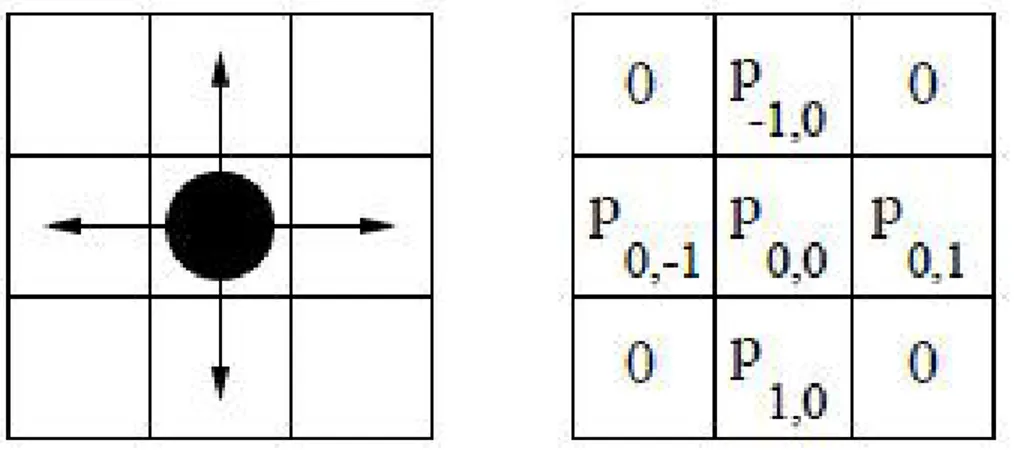
The use of cells forcibly discretizes both space and time : pedestrians can only be located within a cell (which in turn can only fit a single individual) and the smallest meaningful unit of time is therefore the shortest time required to moving between two adjacent cells. At each time step, the new location of each pedestrian is calculated in parallel, the probability of entering a given adjacent cell being a function of the rules within a von Neumann neighborhood (Blue and Adler, 2001, see figure 2.2).
Figure 2.2 A pedestrian, its possible directions of motion, and corresponding probabilities for the case of a von Neumann neighborhood. Source : Sahaleh et al. (2012).
Such models originally had relatively simple rules, largely defining impossible motion (e.g. pedestrians may not walk through each other unimpeded, though they may exchange places) and some fundamental elements of pedestrian motion (e.g. side stepping, preferred speed and collision avoidance). It has since been expanded to include additional behaviors, most
notably the ability of particles to move opposite their preferred direction if necessary (Weifeng et al., 2003), to move obliquely (Yamamoto et al., 2007) and to consider data beyond their immediate vicinity (Burstedde et al., 2001).
It should be noted that while these models are built solely on microscopic interaction and movement and are near-universally considered microscopic models, they have only been va-lidated on macroscopic scales.
2.1.4 Mesoscopic models
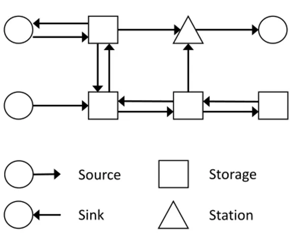
Mesoscopic models stem primarily from the desire to improve upon the computation times involved in microscopic simulation, without sacrificing the ability to account for individual pedestrians (vital in the accurate evaluation of evacuation times). Indeed, early mesoscopic models (such as Hanisch et al., 2003) were aimed at short-term planning and safety in public buildings.
Source Sink
Storage Station
Figure 2.3 Example network used in early mesoscopic models. Inspired by Hanisch et al. (2003).
Such early efforts achieved their goals by first simpli-fying the simulation area into a network of links and nodes (see figure 2.3). The nodes represent either en-trances, exits, stations (where pedestrians must wait to be processed, e.g. a ticket booth) and storage areas, which may be stairways, elevators, hallway intersections, or simply rooms. Pedestrians exist in-dividually within nodes, but are joined into homoge-neous groups in order to move between them ; they are again free to leave and join new groups at sub-sequent nodes. In short, obstacles are modelled by limiting flow out of nodes, and travel times are re-presented by link length.
Hanisch’s model is adequate if pedestrian flow is controlled primarily by bottlenecks connected by hi-gher capacity corridors, as is the case when
move-ment is predominantly unidirectional. It however neglects interpedestrian interactions beyond those in queues, and so cannot readily be applied to more complex cases.
A more generalizable mesoscopic model is that of Teknomo and Gerilla (2008). It funda-mentally resemble cellular automata models, in that the modelled area is decomposed into a lattice of cells, with individuals selecting adjacent cells to move to, much as in figure 2.2.
However, the cells are larger - one to three meters wide - and can therefore accommodate multiple pedestrians. Time to traverse a cell depends on both the trajectory (the source and destination cells) and its current population.
The need to identify and avoid individual collisions is thus elegantly circumvented (at the expense of detailed visualization) but is replaced with a heavy reliance on the accuracy of the fundamental diagram used. A single diagram was utilized in Tekmono et al.’s original paper ; however, fundamental diagrams have been observed to vary by culture (Chattaraj et al., 2009), activity, and type of flow (unidirectional, opposing directions, crossing at various angles, merging, etc.) (Zhang et al., 2011). A greater understanding of the fundamental diagram is hence needed if this model is to more accurately reflect real, complex movement. Qiu and Hu (2013) developed a more fluid, spatial activity-based model. The approach bor-ders on being fully microscopic, as all pedestrians make decisions individually. However, in contrast to the microscopic models presented below, where decisions are made at every time step, decisions in Qui and Hu’s model are made only when a pedestrian moves a threshold distance from (or demonstrates significant activity since) the last decision. Between deci-sions, pedestrians close to one another and with similar directions are grouped together, with characteristics of the group being defined by those of the individuals within it. The model may therefore account for pedestrian heterogeneity in desired speed while maintaining computational performance on par with other mesoscopic approaches.
2.1.5 Discrete choice models
The models discussed thus far were all majoritarily calibrated using macroscopic data ; their microscopic elements (e.g. pedestrian interaction) were designed through observation and adjusted to fit said data. Noting this, Antonini et al. (2004) devised the discrete choice model based solely on microscopic data, established manually from video recordings.
In this model, utilized by the SimPed simulation tool (Daamen, 2002), a pedestrian at a given time t is assumed to make two choices regulating his position at t+1 : one regarding speed (accelerate, decelerate, or maintain the current speed) and the other regarding direction (keep the current heading or turn at predefined, discrete angles). The potential positions resulting from these options form a cone, demonstrated in figure 2.4.
Possible positions are described by several attributes, dependent on proximity to the destina-tion, the presence of obstacles, and both the position and direction of other pedestrians. The pedestrian herself is defined by desired speed and its elasticity, or willingness to diverge from the said speed. Finally, a random variable is implemented in order to capture any otherwise
Decelerate Accelerate Constant Speed
Figure 2.4 Discretization of space based on 3 speed regimes and 7 radial directions. Inspired by Antonini et al. (2004).
unconsidered factors. The probability to enter a given space is defined by the utility func-tion of these attributes, forming a behavioral nested logit model for the operafunc-tional level of pedestrian movement, which is then fitted to the microscopic data. A separate and similar -albeit simpler - model is used to determine paths at the tactical level.
A notable strength of this model is its capacity to accommodate additional variables, and thus take into account factors beyond those stipulated in the original formulation. Indeed, further work has sought to include variables such as visibility (Guo et al., 2012) and density (Asano et al., 2010) as well as improve the ability of simulated agents to identify optimal routes when impeded by other pedestrians (Kretz et al., 2011, notable for using virtual reality to generate a variety of cases for the single test subject). Unfortunately, the primary weakness of logit models is the reliance on large quantities of accurate data ; most (if not all) work on pedestrian discrete choice models has been built on relatively small datasets, most of them experimental.
2.1.6 Social force model
Where the discrete choice models ascribe route-choice to pedestrian agency, the social force model (first described in Helbing and Molnar, 1995) describes pedestrians as passive entities subject to attractive and repulsive forces in their environment. Consequently, a pedestrian’s movement in the model is defined by their acceleration, given by Newton’s equation :
d−→να
dt = − →
The fluctuations term denotes random, unsystematic variations in behavior, representing the fact that pedestrians rarely move in perfectly straight lines. −→Fα(t) denotes the force affecting
the pedestrian at time t and is the sum of the individual, eponymous social forces.
As stated earlier, these forces can be either attractive or repulsive. The former are most prominently exerted by the pedestrian’s destination, though they may also represent objects that will facilitate their journey (such as escalators or signs) or even elements that simply attract attention (e.g. a store display or vending machine). It is therefore possible for the model to account for operational and tactical decisions simultaneously, potentially capturing a realistic, less mechanical set of behaviors : a simulated agent may decide to purchase a coffee before standing at the portion of the platform closest to a television screen, despite the only input order being "board the next train".
Similarly, the repulsive forces mostly define collision avoidance, being exerted by the nearest walls, by obstacles and by most other pedestrians (friends and street artists being possible exceptions). The use of distance-dependent forces in lieu of physical limits allows for micro-scopic behavior more in line with common observations : for instance, when crossing another pedestrian in a hallway, one tends to maintain some near-equal distance from both the cros-sing person and the wall, despite this generally being a slightly longer path than is strictly required.
Evidently, the forces have additional differences. It makes little sense for attraction to the primary destination to vary markedly over time, and it is equally far-fetched to expect an individual to be much distracted by a display too distant to discern. A pedestrian is also less likely to concern herself with the current position of another than with the predicted position at the time of closest approach, and may realistically assume the other will similarly adjust their course (Lakoba et al. (2005) and Zanlungo et al. (2011)). Together, such considerations call for unique formulations for each types of force, additionally variable between individuals in a given population. Consequently, substantial calibration has been required.
At the macroscopic scale, the social force model has been calibrated and validated in a number of cases (Kretz et al. (2008), Beutin (2012)) and is in widespread use for pedestrian simulation, being the core of both VISSIM’s VISWalk and SIMWALK. However, beyond confirming a "natural [...] look and feel of the individual agents" (Kretz et al., 2008) it has not been microscopically validated. Hopefully, as with the other models present here, the availability of additional, real microscopic data will allow further calibration.
2.2 Data collection methods
2.2.1 Point and line data-collection methods
As can be infered from section 2.1, the majority of published pedestrian flow data is macro-scopic. At this scale, the information of interest is speed, density, and volume, at and between points or linear thesholds in the studied network. The simplest and earliest methods were, unsurprisingly, manual, performed by tally sheet or mechanical or electronic count board. Henderson (1974) collected students’ velocities with only a stopwatch and knowledge of the distances travelled. Seyfried et al. (2005a) experimentally studied the density-velocity rela-tionship in single-file queue movement, recording when each individual crossed two predefined screenlines (see figure 2.5). Volume is still routinely collected via manual count, as is density provided an aerial view is available. These methods are simple and reliable, particularly when performed with recorded data (field observers have been found to underestimate volumes by up do twenty-five percent ; see Diogenes et al., 2007) but are costly and cannot easily be em-ployed over long periods of time. Unfortunately, in the cases of density and velocity, manual data collection currently remains the only macroscopic measurement method.
Figure 2.5 Example of a macroscopic pedestrian study, with data collected manually from recorded footage. The time each of the two screenlines (the red vertical lines) is crossed by a pedestrian is recorded manually, allowing both velocity and density measurement. Source : Seyfried et al. (2005b).
In contrast to manually recorded data, automated methods can often be left in place near-indefinitely and at little cost beyond the initial investment. The most typically encountered example is the turnstile, increasingly networked and coupled with electronic transit passes. Though the collected data is often limited to the point of entry alone, in certain cases -most notably, transfer hubs in public transit networks - they can provide a near complete picture of flow volume for an area. The primary drawbacks are that this data is most-often privately owned, and thus seldom made publically available, and that the impediment caused by turnstiles makes their implementation solely for the purpose of counts catastrophically impractical.
A number of more workable pedestrian counting methods exist ; they are well summarized in Bu et al. (2007) :
– Infra-red beam counters : An IR emitter and receiver are placed on opposite sides of a walkway ; pedestrians interrupting the beam between them are counted. While inexpensive, these cannot differentiate between pedestrians and other obstructions, nor can they detect pedestrians occluded by others.
– Passive infra-red counters : Based on military technology, these counters passively de-tects the heat emitted by moving objects within four meters ; models with two detectors can also provide directional counts. They have a particularly high error-rate at higher densities (Kerridge et al., 2004), but these errors are relatively systematic ; with adequate upward adjustments, the resultant counts provide a reasonable estimate of pedestrian vo-lume (Greene-Roesel et al., 2008).
– Piezoelectric pads : A piezoelectric pad is a simple sensor that emits a signal when sufficient pressure is applied. At low densities and when installed where direct physical contact is assured (e.g. a building entrance) they can provide excellent results, and some models even include timer systems to ensure a single count even if two steps are detected from the same individual. However, they are much less effective when multiple pedestrians cross simultaneously.
– Laser scanners : These detectors consist of infra-red laser range finders, which sweep a horizontal or vertical space to detect obstructions - functionally a 360 degree beam counter where the receiver is any static surface. Installed on a ceiling and used vertically, they can provide directional counts through a threshold as well as classify pedestrians by height. Installed at floor level (so as to minimize occlusion) they can detect and even accurately track pedestrians in a space limited primarily by line-of-sight (Zhao and Shibasaki, 2005). Their main disadvantage is their cost, far higher than the other counters in this list, due in large part to the complex signal processing requiring a dedicated processor.
One final automated counting method listed by Bu et al. is using computer vision. If counting is the sole objective, the number of pedestrians can be determined by detection of human-like shapes in still images (extracted or not from video data). While it is also possible (and indeed performed in section 5.1.4) to obtain counts from video data directly by applying video tracking and counting the resultant tracks, this is less a question of macroscopic data collection than one of aggregating microscopic data.
2.2.2 Experimental spatial methods
Figure 2.6 Microscopic video tracking using colored uniforms as visual cues. Source : Hoogendoorn et al. (2003a). Experimental settings allow the researcher nearly
complete control over the pedestrian environment. In addition to allowing the examination of specific circumstances and their effects on pedestrian flow, such settings greatly facilitate the accurate extrac-tion of pedestrian trajectories by permitting a broa-der number of tracking methods than are available in the field. Said methods are too numerous and va-ried to exhaustively list here. However, they can be summarily categorized for the purposes of this study into video-based and non-video-based methods. Generally, the simplest way to track pedestrians mi-croscopically without resorting to video recording is to give them a tracking device. These can range from inertial sensors (e.g. Feliz Alonso et al. (2009), Fox-lin (2005)) to the augmented-reality headset used by Kretz et al. (see section 2.1.5), but such devices
are costly to provide to more than a handful of pedestrians. This may be circumvented by the increasing ubiquity of smartphones, and wearable technology may eventually allow more generalizable tracking through triangulation of the emitted wireless signals : Danalet et al. (2014) managed to accurately track the activity of a subject throughout a university campus from network traces. At present, however, these methods are limited to very specific appli-cations : despite the increasing ubiquity of personal wireless devices, there is no guarantee any given individual will carry the device through every movement, nor that it will be set to transmit on the frequency used for tracking.