Nondestructive testing of metals and composite materials using ultrasound thermography : comparison with pulse-echo ultrasonics

Nondestructive testing of metals and composite

materials using ultrasound thermography:

Comparison with pulse-echo ultrasonics

Mémoire présenté

à la Faculté des études supérieures et postdoctorales de l'Université Laval dans le cadre du programme de maîtrise en génie électrique

pour l'obtention du grade de Maître es sciences (M.Sc.)

DEPARTEMENT DE GENIE ELECTRIQUE ET DE GENIE INFORMATIQUE FACULTÉ DES SCIENCES ET DE GÉNIE

UNIVERSITÉ LAVAL QUÉBEC

2012

La thermographie stimulée par ultrasons (TU) est une méthode de contrôle non destructif qui a été inventée en 1979 mais qui a s'est répandue à la fin des années 90. L'idée de cette méthode est d'exciter le matériau à inspecter avec des ondes mécaniques à des fréquences allant de 20kHz à 40kHz et d'observer ensuite leur température de surface avec une caméra infrarouge. TU est une méthode de thermographie active; les autres méthodes les plus connues sont la thermographie optique et celle stimulée par courants de Foucault. Son habilité à révéler des défauts dans des cas où les autres techniques échouent, fait d'elle une méthode pertinente ou complémentaire. L'inconvénient de la TU est que beaucoup de conditions expérimentales doivent être respectées pour obtenir des résultats adéquats incluant quelques paramètres qui doivent être bien choisis.

Le but de ce projet est d'explorer les capacités, les avantages et les limites de la TU. Pour comparer la performance de la TU à celle des ultrasons conventionnels, des tests ultrasons de type C-Scan ont été réalisés pour quelques échantillons. Quatre matériaux différents avec quatre types de défauts ont été investigués afin de mieux définir les conditions optimales pour améliorer la détection des défauts. Les résultats bruts obtenus étaient traités dans chaque cas afin de mieux visualiser les contrastes thermiques causés par les discontinuités cachées.

Ultrasound thermography (UT) is a nondestructive testing method that was invented in 1979 but became widespread in the late 90s. The idea of this method is to excite the material under test with mechanical waves of high frequency (20kHz - 40kHz) and to observe the surface temperature profile with a high-speed infrared camera. UT is an active infrared thermography method; other renowned methods are optical and eddy-current thermography. Its unique ability to reveal defects in cases where other techniques do not perform well makes it irreplaceable or complementary. The drawback of UT is that a long list of experimental conditions must be respected, including several parameters that must be properly chosen to produce adequate results.

The aim of this project is to define the capabilities of UT, to confirm/refute and extend its advantages and limitations. In order to compare the performance of UT to that of ultrasonic testing, C-scans were conducted for some specimens. Four different materials with four types of defects were investigated to define the optimal experimental conditions for optimal defect detection. Obtained raw results were processed using appropriate image processing techniques that made representation about their efficiency in each case.

Acknowledgment

First of all, I would like to thank my supervisor Abdelhakim Bendada and co-supervisor Xavier Maldague for their support and encouragement during this master program. I really appreciate their contribution and advice on my research work, and the knowledge that they gave me in class.

I am also grateful to Clémente Ibarra-Castanedo, Matthieu Klein and Marc Grenier for their collaboration in theoretical and practical aspects of NDT and thermography in particular. Thanks go also to Denis Ouellet for his will to help with any question on informatics or the equipment part, and to Marco Béland for his help in specimens' production.

Finally, I would like to thank my colleagues, Frank Billy Djupkep Dizeu, Yuxia Duan, Reza Shoja Ghiass, who always supported my work, and made these two years pleasant, adventurous and memorable.

Table of Contents

Résumé i Abstract ii Acknowledgment iii

List of equations vii List of figures viii List of tables x Introduction 1 Chapter 1 Nondestructive testing 3

1.1. Liquid penetrant testing 3 1.2. Ultrasonic testing 4 1.3. Radiographic testing 4 1.4. Magnetic particle testing 5 Chapter 2 Infrared thermography 7

2.1. Physical basics 7 2.1.1 Infrared radiation 7 2.1.2 Plank's law 8 2.1.3 Emissivity 9 2.2. Infrared system 10 2.3. Infrared thermography as an NDT method 11

2.3.1. Classification 11 2.3.2. Advantages and limitations 13

2.3.3. Applications 13 Chapter 3 Ultrasound thermography 15

3.1. Sonic/ultrasound thermography development timeline 15

3.2. Physical basics 17 3.2.1. Sound 17 3.2.2. Thermal phenomena 21

3.3. Experimental setup and possible configurations 22

3.5.1. Fast Fourier Transform 26 3.5.2. Principal components thermography 27

3.6. Mathematical modeling and computer simulations 29 Chapter 4 Equipment and experimentation parameters 31

4.1. Ultrasound thermography setup 31

4.1.1. Acquisition system 32 4.1.2. Source of ultrasounds 34 4.1.3. Branson 2000LPt 34 4.1.4. Branson 2000b 34 4.1.5. Laser vibrometer 37 4.1.6. Coupling and isolation materials 40

4.2. Ultrasonic testing setup 41

4.2.1. Water bath 41 4.2.2. System of axis XY 42

4.2.3. Flaw detector OmniScan MX UT 42

Chapter 5 Experimental results 43

5.1. CFRP specimens 43 5.1.1. Description of specimens and defect production 44

5.1.2. Experiment 45 5.1.3. Results and discussion 46

5.2. Steel specimen 62 5.2.1. Description of a specimen and defect production 62

5.2.2. Experiment 63 5.2.3. Results and discussion 64

5.3. Aluminum specimen 66 5.3.1. Description of the specimen and defect production 66

5.3.2. Experiment 66 5.3.3. Results and discussion 67

5.4. Plexiglas specimen 72 5.4.1. Description of the specimen and defects production 72

5.4.2. Experiment 73 5.4.3. Results and discussion 74

Chapter 6 Conclusion SI

Bibliography 83 Appendix 1: Technical data of IR camera Phoenix Indigo 87

Appendix 2: Technical data of Branson 2000LPt 88 Appendix 3: Technical data of Branson 2000b 92 Appendix 4: Technical data of the Polytec laser vibrometer 93

Appendix 5: Technical data of OmniScan MX UT 95 Appendix 6: Technical features of the used black paints 96 Appendix 7: Ultrasound Thermography setup tutorial 97

List of equations

Equation 2.1: Planck's law I Equation 2.2: Spectral radiance 9 Equation 3.1: Snell's law 19 Equation 3.2: Generated thermal signal 22

Equation 3.3: Discrete Fourier transform 26 Equation 3.4: Amplitude from FFT 26 Equation 3.5: Phase from FFT 26 Equation 3.6: PCT matrix 27 Equation 3.7: Signal-to-noise ratio 27

Equation 4.1: Doppler frequency 38 Equation 4.2: Acoustic impedance of coupling material [46] 41

List of figures

Figure 1.1: Liquid penetrant technique 3 Figure 1.2: Ultrasonic testing technique [2] 4 Figure 1.3: Radiographic testing technique [2] 5 Figure 1.4: Magnetic particle testing technique [2] 5

Figure 2.1: Electromagnetic spectrum [3] 7 Figure 2.2: Spectral radiance of a blackbody [4] 9 Figure 2.3: Spectral emissivity of some materials [6] 10 Figure 2.4: Block diagram of a radiation pyrometer 10

Figure 2.5: IR thermography methods 12 Figure 3.1: Frequency ranges of sound 18 Figure 3.2: Reflection and refraction at the boundary between two media [29] 19

Figure 3.3: Piezoelectric effect [30] 20 Figure 3.4: Experimental setup for ultrasound thermography [33] 23

Figure 3.5: Amplitude modulated signal 23

Figure 3.6: Burst signal 24 Figure 3.7: Frequency modulated signal (chirp) [34] 24

Figure 3.8: Response at peak contrast [39] 27 Figure 3.9: Peak contrast distribution and first four EOFs [39] 28

Figure 4.1: Ultrasound thermography setup 31 Figure 4.2: Measurement of vibration characteristics 32

Figure 4.3: RTools software 33 Figure 4.4: Graphique user interface for Branson 2000LPt [33] 34

Figure 4.5: Graphical user interface Branson UPS 36 Figure 4.6: Graphical user interface for Branson 2000TLPt [33] 36

Figure 4.7: Examples of modulating signals and corresponding frequency-modulated

waveforms: a) Ramp modulating signal; b) Periodic modulating signal. [44] 37

Figure 4.8: Modules of the laser-Doppler vibrometer [45] 37 Figure 4.9: Velocity of specimen excited on 20kHz during 80ms 38

Figure 4.11: Specimen clamping 40 Figure 4.12: Scheme of impedances 40 Figure 4.13: Water bath and system of axes 41

Figure 4.14: Connection of control elements 42

Figure 4.15: OmniScan MX UT 42 Figure 5.1: Specimens #4 and #5 44 Figure 5.2: Specimens #1, #2, #3 45 Figure 5.3: CFRP specimen fixation 45

Figure 5.4: Specimen #4 47 Figure 5.5: Specimen #4, temperature profiles in the defect areas 48

Figure 5.6: Specimen #4, C-Scan 49 Figure 5.7: Specimen #4, A-Scan in six points 51

Figure 5.8: Specimen #5 53 Figure 5.9: Specimen #5, temperature profiles in defect areas 54

Figure 5.10: Specimen #5, C-Scan 55 Figure 5.11: Specimen #5, A-Scan in six points 57

Figure 5.12: Specimen #1 59 Figure 5.13: Specimen #1, temperature profiles in defective and sound areas 60

Figure 5.14: Steel specimen 62 Figure 5.15: Steel specimen fixation 63

Figure 5.16: Steel specimen 65 Figure 5.17: Aluminum specimen 66 Figure 5.18: Aluminum specimen fixation 67

Figure 5.19: Aluminum specimen 68 Figure 5.20: Temperature vs. time (lock-in) 68

Figure 5.21: Temperature vs. frequency (lock-in) 69 Figure 5.22: Thermal image of the crack (lock-in) 69

Figure 5.23: Temperature vs. time (burst) 70 Figure 5.24: Temperature vs. frequency (burst) 70 Figure 5.25: Images of the crack (burst) 71

Figure 5.27: Plexiglas specimen fixation 73

Figure 5.28: Plexiglas specimen (lock-in, without horn) 74 Figure 5.29: Plexiglas specimen fixation with horn 75 Figure 5.30: Plexiglas specimen (burst, with horn) 76 Figure 5.31: Temperature contrast profile (burst, with horn) 76

Figure 5.32: Plexiglas specimen (lock-in) 78 Figure 5.33: Temperature contrast profile (lock-in) 78

List of tables

Table 5.1: Maximum temperature contrast values (burst) 77 Table 5.2: Maximum temperature contrast values (lock-in) 79

With the onrush of science and technology nowadays, the specified requirements for quality products become stricter. The invention of new materials and the extension of their fields of application require special methods for defect detection.

There is an important group of methods, called Nondestructive Testing (NDT) methods, in which materials and structures may be inspected without disruption or impairment of their serviceability. One of these methods is ultrasound thermography (UT) based on two physical principles: excitation of the specimen by high-frequency mechanical waves (ultrasound) and observation of the surface temperature by infrared vision.

The Computer Vision and Systems Laboratory (LVSN) of Laval University has an ultrasound thermography setup and a bank of specimens containing various natural or artificially produced defects.

The first chapter of this work contains general information about NDT and four most commonly used methods: liquid penetrant, ultrasonic, radiographic and magnetic particle testing. A detailed description of IR thermography is presented in the second chapter. There are physical basics, classification of IR techniques, advantages and limitations, and application of these methods. The third chapter is dedicated to ultrasound thermography, with its physical fundamentals, characteristics, history of development. Apparatus and experimentation details are described in chapter four. In the fifth chapter, descriptions of the specimens, experimental results, and their analysis are presented. The thesis concludes in chapter six with a synopsis and a discussion of future work.

The main objective of NDT is to detect the defects in a sample at the stage of its production or during its utilisation. So we can avoid breakdowns, prevent accidents, and ensure customer satisfaction.

There is a wide variety of NDT methods: visual, eddy current, liquid penetrant, ultrasonic, radiographic, leak testing, acoustic emission, magnetic particle inspections and infrared testing [1]. Every method has its own advantages and disadvantages. According to the measurement conditions, such as type of material, nature, depth, and size of defect, inspection speed or others, one or another NDT method is preferred.

1.1. Liquid penetrant testing

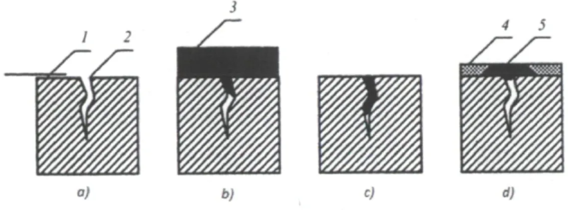
The liquid penetrant testing is one of the oldest methods of NDT. It is based on a penetrant seeping into the surface defects or to subsurface defects with surface openings. The steps of penetrant inspection are shown in Figure 1.1. Firstly, the surface to be inspected (1) is cleaned from all traces of dirt and grease (a). Then a liquid penetrant (3) is applied to it (b). After the penetrating period, usually about 20 minutes, the remaining penetrant is removed from the surface (c). Then an absorbent, light colored powdered material, called a developer (4), is applied (d). This developer soaks up a portion of the penetrant from the opening (2) and the outstanding area (5), the location of the defect, can be easily visible by the naked eye or through the special ultraviolet illumination.

3 1 2

o) b) à)

This method is based on sound wave propagation and reflection in materials; thus, an ultrasound transducer employs high frequency (0.5MHz - 25MHz) sound pulses which propagate into the sample, reach an interface and travel back to the surface. Reflected waves are collected by an analog or digital detector and displayed on a monitor as a series of signals. The presence of the defect will cause changes in the amplitude of responses.

Transducer generates and receives S o u n d p a t h Defect Generating signal Receiving signal _{— — £ — i=}

Figure 1.2: Ultrasonic testing technique [2]

1.3. Radiographic testing

Radiography allows to obtain the image of material's internal defects (especially volumetric) by X-rays. In this technique the test object is placed between the radiation source and the detector (film or other radiation sensitive material). Travelling through the material, the intensity of the ionization radiation changes depending on the thickness of the material and the presence of defects. The resulting image is developed on the detector (Figure 1.3).

Pilm

Darkened area (when processed)

Figure 1.3: Radiographic testing technique [2]

1.4. Magnetic particle testing

It is the most commonly used method for crack detection in ferromagnetic materials. Cracks can be opened or be located just below the surface. The surface is covered by metal iron dust. When a magnetic flux flows through the material, dust particles are concentrated near the crack. This method allows one to determine the crack location but does not provide information about its depth. Fluorescent particles can be used for better visibility. The sensitivity of this method strongly depends on the surface quality.

Magnetic particles

Magnetic field

Figure 1.4: Magnetic particle testing technique [2]

The next chapter describes the physical basics, various methods and other features of Infrared thermography.

2.1. Physical basics

2.1.1 Infrared radiation

A German astronomer, W. Herschel, in 1800 discovered the existence of infrared rays during his experiment with a glass prism and thermometers. While moving the thermometers, he measured the temperature in each colour zone. He found that temperature was increasing from the violet to the red part of the spectrum. When he moved the thermometer beyond the red part, he found that this region had the highest temperature. Thus, he made a great discovery and this part of the spectrum was named "infrared radiation". Hence, infrared radiation is electromagnetic radiation covering the spectral region between the red end of visible light (X ~ 0.7u.m) and microwaves (k ~ 1000|xm) (Figure 2.1).

There are three bands of infrared radiation - near infrared (NIR), mid infrared (MIR) and far infrared (FIR), but specialists of different fields define different borders between them.

Here is one of those divisions (ISO 20473): • near infrared - 0.78 - 3 pm;

• mid infrared - 3 - 50 um; • far infrared - 50 - 1000 um.

Another way to classify the IR band is according to the spectral sensitivity of the camera. For instance:

• near infrared (NIR) - 0.78 - 1 jam; • short-wave infrared (SWIR) - 1- 3 um; • mid-wave infrared (MWIR) - 3 - 5 um; • long-wave infrared (LWIR) - 7.5 - 14 |am.

2.1.2 Plank's law

Thermography generates images (thermograms) where the contrast is provided by local thermal emission. The law governing thermal emission is the Planck's law. It describes the distribution of emitted energy as a function of the wavelength (I) for a given blackbody

temperature (T).

2hc2 Equation 2.1: Planck's law

Lx,b (-*- T) = -jp

d \ em -1)

Where h - Planck's constant (6.626076xlO"34Js);

c - Speed of light (~3><108 ms"1);

Figure 2.2: Spectral radiance of a blackbody [4]

2.1.3 Emissivity

The emissivity of material is the relative ability of its surface to emit energy by radiation. It is the ratio of the energy radiated by a particular material to the energy radiated by a blackbody at the same temperature. A blackbody is a hypothetical body that absorbs, without reflection or transmission, all of the electromagnetic radiation falling upon it and that yields the maximum radiation energy theoretically possible at a given temperature. The emissivity of blackbody is 1.0, while for all other materials it varies from 0 to 1.0 (Figure 2.3). Emissivity depends on the surface orientation, temperature and wavelength. Surfaces with a low emissivity (polished metals, for example) act as a mirror. It is then difficult to measure the real temperature of a sample surface because of the influence of emitted radiations from the surrounding objects. There are several ways to reduce the impact of the environmental reflections. One of them is to cover the inspected surface with a high emissivity flat paint (with s ~ 0.95) [5].

1 0

i J

f

i J

f

K^S

f

f

f

Figure 2.3: Spectral emissivity of some materials [6]

2.2. Infrared system

The infrared system consists of five components: the optical system, the detector, the amplifier, the signal processing block and the display. As an example, a radiation pyrometer is presented in Figure 2.4. Object Detector — y Adjustable Eyepiece Amplifier __$, Signal processing ___£> Display

.An optical system collects the visible and infrared energy from an object and focuses it onto a detector. The detector converts this energy into an electrical signal which then is processed and displayed as a value of measured temperature.

There are two main types of detectors: thermal (bolometer, microbolometer, thermopile and pyroelectric detector) and photonic (quantum) (photoconductive, photoemissive and photovoltaic detectors).

Thermal detectors are based on the temperature dependent phenomena (temperature change, thermoelectric effect, etc.). They are practically independent on the wavelength, the element does not need to be cooled and their price is comparatively low. In photonic detectors the electrical signal is obtained by measuring the quantity of incoming photons. Their response time and sensitivity are much higher but usually they must be cooled to avoid the thermal noise. Furthermore, their sensitivity depends on the wavelength.

2.3. Infrared thermography as an NDT method

Infrared thermography (IR thermography) is one a widely used technique, which enables inspection of large areas in a fast and safe manner. Its principle is to measure surface temperature variations of a component. A temperature contrast is created and detected by the infrared camera over defective areas of the specimen.

2.3.1. Classification

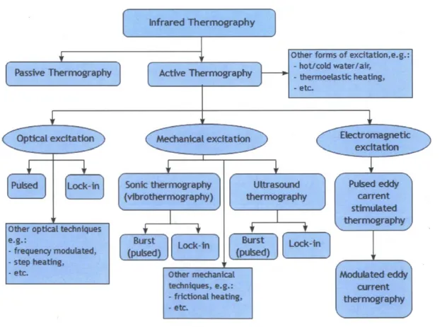
Several types of IR thermography are known nowadays (Figure 2.5). They can be classified into two groups based on the temperature difference generated to obtain a thermal image: passive thermography and active thermography. The passive thermography is used for the objects which are naturally at the higher temperature than ambient. In the case of active thermography, an external energy source (hot or cold) is introduced to generate the relevant temperature difference.

Active thermography can be classified by the mode of thermal stimulation: pulsed thermography, lock-in thermography, step heating, etc.

Pulsed thermography (PT) is when the specimen surface is exposed to a short heat pulse. Lock-in thermography (LT) is when harmonic stress waves are applied to a specimen surface.

Step heating (SH) is when the surface is exposed to a stepped heating pulse ("long pulse") at low power.

There are several types of external energy sources which can be used for specimen heating: optical (photographic flash, halogen lamps, etc.), mechanical (sonic or ultrasonic transducer), electromagnetic, etc [7].

Infrared Thermography

JL

Passive Thermography

Optical excitation

Pulsed Lock-in

Other optical techniques e.g.:

- frequency modulated,

- step heating, - etc.

Active Thermography

Other forms of excitation,e.g.: - hot/cold water/air,

- thermoelastic heating, - etc.

Mechanical excitation Etectromagnetic excitation Sonic thermography ( vibro thermography )

c

F

2.3.2. Advantages and limitations

There are many advantages of IR thermography that makes it more competitive as compared to other NDT methods:

• fast, reliable and accurate output;

• a large surface area can be scanned rapidly; • no contact needed;

• secure for users (no harmful radiation);

• can be applied for both curved and flat surfaces; • presented in visual and digital form;

• it is possible to examine the sample only on one side; • can be used to detect objects in dark areas;

• software for image processing and analysis are available.1

There are also some limitations to IR thermography:

• ability to inspect a limited thickness of material under the surface; • reflections from surrounding surfaces can influence the result;

• high price range of equipment, although prices are constantly falling.

2.3.3. Applications

Passive thermography is usually used for predictive and preventive maintenance (e.g. crack or corrosion detection in oil & gas pipes, train wheel inspection, electrical maintenance, etc.) while the active one is most useful when more detailed information about the internal structure of a test object is needed.

Active IR thermography has been successfully applied for detection of delaminations and disbonds in layered structures, hidden corrosion in metallic components, cracks in ceramics and metals, voids, impact damage and inclusions in composite materials, etc.

The next chapter discusses the fundamentals of ultrasound thermography.

Chapter 3 Ultrasound thermography

When using mechanical excitation sources like electromagnetic or piezoelectric transducers on frequencies up to 20kHz, the method is called sonic thermography, on frequencies 20kHz to 50kHz, it is called ultrasound thermography (UT).

These methods use high-speed, full-field infrared imaging to detect cracks, delaminations or other defects both surface and subsurface. A short pulse (burst) or a wave of sound is applied to a structure. Due to the thermal phenomena - thermoelastic effect and hysteresis (loss angle), mechanical energy is converted into thermal waves locally at the interface of a defect, then heat travels to the surface. The tempéramre increases in the vicinity of the defect and this local increase becomes visible by the IR camera.

3.1. Sonic/ultrasound thermography development timeline

The defect detection technique using mechanical vibrations was first reported in 1979 by Henneke [8] in the USA. Various sample types (laminates, metals and polymers) were investigated. As a source of mechanical energy a transducer of 1 - 20kHz was used, as a measuring instrument an IR camera AGA Thermovision Model 680 [8-10]. Shortly after Henneke's first experiments, British researchers, Pye and Adams [11], made experiments to detect shear cracks in tubes and plates made of glass fibre reinforced plastic (GFRP) and carbon fibre reinforced plastic (CFRP), using resonant vibration. For each sample they chose an appropriate resonant frequency that allowed them to create greater stresses in the structures using lower-power devices [11].

Since then, many investigators have studied the application possibilities, efficiency and other aspects of sonic/ultrasound thermography. Rantala and Busse, 1996 [12] invented a new technique - lock-in vibrothermography. Using it they made a series of experiments to detect various defect types in polymer and composite materials. As a result, it was found that this method is effective in that type of applications, and especially suitable for detection of small delaminations and cracks in CFRP with long fibers [12, 13].

ultrasound lock-in thermography for the inspection of several materials. During the experiments they successfully detected vertical cracks in a steel sample, in ceramic materials and C/SiC plates; corrosion in aluminum plates; cracks and delaminations in stringer structures; cracks along rivets; impact damages, resin bridges between top and bottom layer and metal inserts in the foam layer at various depths in a sandwich structure that consisted of a polymer foam between two thin CFRP layers.

Favro et al., 2000 [18] presented a new technique of ultrasound thermography - burst (sonic pulse) thermography. For their experiments they used aluminum alloy bars containing fatigue cracks and a graphite fiber reinforced polymer composite containing interply delaminations. This technique also proved the efficiency of ultrasound excitation application for detection of cracks with non-planar geometrical orientation.

In 2002 a group of researchers from Wayne State University, USA - Han, Favro, and Thomas [19], were the first to describe a quasichaotic mechanism for the generation of complex vibrations. Measuring the frequency pattern of a sample, while inducing mechanical waves in it, they found additional frequencies, subharmonics of the main one. Later, in 2003, they assumed the ability of acoustic chaos to enhance crack detectability while using the technique of sonic infrared imaging. Through a series of experiments on an aircraft engine disk with shallow cracks and other aluminum plates, using nonchaotic, chaotic and low-power chaotic wave excitation forms, their hypothesis was confirmed [20]. Afterwards, Han et al. [21, 22] performed mechanical and finite-element models in which chaotic effects, including the appearance of additional frequencies, result from the interaction between the ultrasonic source and the sample.

As the high excitation power contained in bursts may cause damage of the inspected material, one transducer generating a long low-power pulse or several transducers in the same time can be used (Barden et al., 2006 [23]; Zweschper.et al., 2003 [24]). This approach provides a more homogenous low-power density in the sample so that even larger components can be examined with this technique.

measuring system in which instead of an ultrasonic welder a broadband actuator is used (piezoelectric stack driven by a power amplifier fed by an arbitrary waveform generator). The excitation signal is a sweep (chirp) with a frequency 1-20kHz. As the frequency varies, at some point it will match the natural one of a specimen, so resonance will take place. In this case comparatively low power will be sufficient to generate detectable amounts of heat in cracks. In addition, the broadband excitation can be tuned to match the specific resonant frequencies of the specimen, thereby improving the chances of detecting a crack.

In 2008 the first noncontact ultrasound thermography (air coupled acoustic thermography (ACAT)) was implemented by Zalameda et al. [26]. The object of investigation was a sandwich honeycomb structure, helicopter blade section, with ballistic damage to the outer skin and core. The AC AT system consisted of an acoustic source of 800-2000Hz and pulsed at 0.5Hz. By this technique it was possible to detect skin to core disbonds that were not seen with an optical thermography. Another advantage of ACAT is that it is a noncontact technique (no coupling material needed and there is low chance of specimen surface damage). Moreover, it can be useful for large surfaces.

The experiment of Guo et al., 2009 [27] on gas turbine blades with service induced fatigue cracks achieved the highest efficiency of ultrasound thermography in comparison with visual and fluorescent penetrant inspection.

Holland, 2011 [28] improved the method of thermographic signal reconstruction in crack detection using ultrasound thermography. He developed an algorithm that reduces the entire time sequence to a single static plot, improves sensitivity and reduces the noise.

■

3.2. Physical basics

3.2.1. Sound

Sound is an elastic wave that creates mechanical oscillations when propagating through a solid, liquid or gas medium. In liquids and gases acoustic waves have a longitudinal character. It means that the particle oscillation direction is aligned with the direction of

wave propagation. In solid mediums, besides the longitudinal deformations, compliance of displacement exists which causes a transverse wave excitation. In this case, particles oscillate perpendicularly to the direction of wave propagation. The speed of longitudinal wave propagation is much higher than that of the transverse wave.

3.2.1.1. Classification

As every wave, sound is characterized by an amplitude and a frequency range. The human ear is capable of perceiving sounds in 20Hz - 20kHz range. Frequencies < 20Hz correspond to infrasound, 20kHz - 1GHz to ultrasound, and > 1GHz to hypersound (Figure 3.1).

Infrasound Audible sound Ultrasound Hypersound

I 1 I

►

20 Hz 20 kHz 1GHz F, Hz Figure 3.1: Frequency ranges of sound

Infrasound

Infrasound results naturally from severe weather (earthquakes, volcanoes, waterfalls, etc.) or generated by man-made processes (transport, heat-only boiler stations, wind turbines, etc.). Due to its weak absorption in different mediums infrasound can propagate in the air, water and crust over very long distances.

Ultrasound

In the living world ultrasound is a component of many natural noises (wind, waterfall, rain, sounds of thunder etc.) and it is used by animals (bats, whales, certain insects, etc.) for navigation purposes.

In industry, medicine or science, ultrasound is artificially produced by generators. In some of them oscillations are generated by means of a barrier on the way of direct current such as gas or fluid flows. In others by means of electro-acoustic transducers that convert the voltage oscillations into mechanical vibrations of solid object which emit acoustic waves in the material.

Since ultrasonic waves have a relatively short wavelength, even comparatively small sound sources can form narrow beams, so the intensity of ultrasonic oscillation can be high. This fact is the basis of important applications in NDT and medicine.

Hypersound

Natural hypersound is generated by the atomic vibrations of a material. Artificial hypersound is generated by the excitation from the surface of a piezoelectric crystal. Hypersound has the same physical nature as ultrasound but at the molecular level a difference exists. Since, the hypersonic wavelength is almost equal to the mean free path of molecules of air and gases at normal atmospheric pressure these waves do not propagate in them. In liquids the attenuation of hypersound is very high and the propagation range is small. Solids in the form of single crystals are relatively good conductors of hypersound but mainly at low temperatures only.

3.2.1.2. Reflection and refraction

When a sound wave encounters the boundary between two media with different physical properties, it can be partially or even totally reflected. Sometimes a part of the sound comes through the second medium where it changes its direction and velocity. This process is called refraction. Both reflected and refracted waves have amplitude and phase different from the incident wave.

According to the law of reflection the angle of reflection is equal to the angle of incidence (Figure 3.2).For refracted wave the Snell's law is expressed as:

_ _j_a __ • a Equation 3.1: Snell's law

ni sin»! =n2Sin02 Incident Reflected wave wave e« 9l / Refractive jndex - n. Medium 1 Medium 2 6_~~ Refractive index - n2 6_~~ Refracted wave

3.2.1.3. Standing waves

The phenomenon called standing (stationary) wave occurs in the situation of superposition of two waves of the same frequency traveling in the opposite directions. The most common example of standing wave is when the wave propagating through the medium reflects back when it reaches its end.

In the context of NDT this phenomenon can create difficulties in the interpretation of the thermogram because these waves can appear as temperature patterns due to the hysteretic losses in the elongation maximums.

3.2.1.4. Generation of audible sound and ultrasound

Two types of sound transducers exist: electromagnetic and piezoelectric. The electromagnetic (electrodynamic) transducer principle of operation is based on the transformation of electromagnetic energy into mechanical energy using a moving system in a permanent magnetic field coil.

The main part of a piezoelectric transducer is a layer of piezoelectric material sandwiched by thin metal electrodes on both sides. When an alternative electrical voltage is applied, the thickness of the layer is changed proportionally to the value of this voltage; this phenomenon is called "reverse piezoelectric effect" (Figure 3.3). Thus, electrical energy is converted into mechanical vibrations. In order to influence its mechanical resonance, additional mass can be loaded onto the piezoelectric layer.

Due to their high efficiency, simple construction and the uniformity of the exciting force, piezoelectric transducers are the most popular ultrasound sources nowadays.

mechanical __*, ^ * ~ . +.\ ^ electrical energy +~ \ ' >/ _ )*— energy

The most typical example of such material is quartz. Despite the low mechanical and electrical losses and high resistance to electrical breakdown, twinning effects, that change physical properties of crystal, can take place in quartz that reduces the piezoelectric effect. Moreover, this quartz is inexpensive.

Lately, piezoelectric ceramics have been widely used. These materials are synthesized from different powdered matters (usually metal oxides) by mixing them and pressing them at high temperature into desired shape. Thereafter they are poled by electric field at high temperature, and during cooling the dielectric moment is frozen into their structure.

High electromechanical transforming efficiency at the point of resonance, high stability and the possibility to have different shapes make piezoelectric ceramics very popular for mechanical energy or electrical signal generation [31].

3.2.2. Thermal phenomena

In ultrasound thermography, mechanical energy is converted into thermal energy in the zone of the defect. This mechanism is possible by the presence of three principal phenomena: friction, thermoelastic and hysteresis effects.

Friction is a physical phenomenon that occurs when two objects slide along each other. In the case of a crack the two objects are its two surfaces. For a delamination or inclusion of a substantially different density material, the two objects are the contact surfaces of these materials. In both cases mechanical waves propagate into the specimen, force the surfaces to rub against each other. Mechanical energy is thus converted into heat, and the presence of the defect becomes detectable by the IR camera.

This phenomenon makes UT very interesting for NDT applications because the defect detectability does not depend on the orientation of the defect. This is a problem that most NDT techniques are not able to solve. The more important here is the roughness of the two involved surfaces (more rough they are more thermal energy is generated).

Thermoelastic effect describes the relationship between mechanical deformation and temperature change of an elastic material. When a material is being elongated, its

temperature decreases, when it is being compressed its temperature increases (adiabatic conditions are required).

Hysteresis describes the behaviour of the material that is periodically mechanically deformed. The stress-strain diagram is a loop. One of its curves presents the loading, another one unloading, and the enclosed area corresponds to the dissipated energy that was converted into heat. The efficiency of heat generation increases with vibration frequency since more hysteresis loops are generated per unit time. Therefore, it is more useful to use ultrasound.

Mathematically, the generated thermal signal S can be described as:

5 = Kraac + K2Oac Equation 3.2: Generated thermal signal

where aac is a stress amplitude, K] and K2 are complex constants defining the thermoelastic

and the hysteresis effects, respectively [32].

Because of a high acoustical damping even at low amplitudes the hysteresis effect is stronger in polymers than in metals. While in metals the thermoelastic effect dominates.

3.3. Experimental setup and possible configurations

A schematic diagram of the experimental setup for ultrasound thermography is shown in Figure 3.4. A piezoelectric shaker system is used to apply mechanical energy (acoustic wave) into the specimen which has an internal discontinuity. The surface tempéramre of the area under inspection is imaged by an infrared camera which is triggered simultaneously with the shaker system via computer-controlled system to initiate the data acquisition equipment.

Computer l ' I t r u o u n d controller Interna) diwontinuiiy Cuntrul unit A synchronization

H^____>

I

Figure 3.4: Experimental setup for ultrasound thermography [33] In ultrasound thermography two configurations have been mainly introduced:

• Lock-in (amplitude modulated) thermography, in which the high frequency signal is amplitude modulated at a much lower frequency (Figure 3.5); the IR camera is synchronized with the input signal and collects the surface thermal image.

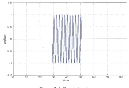
• Burst thermography, in which the sample is excited by a brief (typically 50 -200ms) ultrasonic pulse (Figure 3.6) and the surface temperature, is collected as a function of time, also by an IR camera.

Figure 3.6: Burst signal

It is possible to modulate the frequency in both configurations (Figure 3.7). The procedure, called wobbulation, allows to cover a range of frequencies on a single experiment, instead of only one, since it is not always possible to predict the right frequency for a particular application. Moreover, wobbulation is useful to prevent the appearance of standing waves, which are produced when working at the natural harmonic resonance frequencies of the material [34].

• . 1. . . ._ .

MM|I||

1

villi!

1

3.4. Advantages and limitations

As every technique, ultrasound thermography has its advantages, that makes it useful in some applications where other IRT techniques do not perform well enough. Mainly:

• fast (from a fraction of a second to a few seconds); • allows to detect deeper defects;

• allows to detect closed cracks, nanometric open cracks, vertical cracks, kissing disbonds;

• can be applied to large areas of structures.

But there are also some requirements for ultrasound thermography application: • direct contact between transducer and sample;

• coupling material (for acoustic impedance matching and sample protection); • appropriate pressure of transducer (to avoid damage of the sample);

• appropriate type of excitation (lock-in or burst, with or without frequency modulation);

• appropriate excitation and modulation frequencies and amplitudes;

• the optimal parameters are obtained mostly experimentally with some guidelines from analytical and computer modelling studies.

3.5. Image processing and data analysis

When the raw image is not enough to observe the defect, image processing and data analysis are required. Image processing allows to improve defect contrast, to reduce the impact of non-uniform heating, emissivity variations and environmental reflections.

A great variety of processing techniques have been developed in the infrared community: thermal contrast computations, normalization, Fast Fourier Transform (FFT), Principal Components Thermography (PCT), Thermographic Signal Reconstruction (TSR), etc. For example, FFT allows retrieving phase and amplitude data from the image, TSR considerably reduces the amount of data to be handled, de-noising the signal and allowing the algebraic manipulation of data, etc. [35, 36]. For ultrasound thermography, cold image subtraction is sometimes enough but the best results can be obtained with FFT or PCT.

3.5.1. Fast Fourier Transform

To analyze the thermal response of the specimen in a frequency domain the fast Fourier transform (FFT) is used. FFT is an algorithm to calculate the discrete Fourier transform (DFT) and its inverse.

One-dimensional DFT for each pixel of the thermogram sequence can be described as:

/v-i

Fn = Y T(k)e2nikn'N = Ren + i lm*

Equation 3.3: Discrete Fourier transform

Where i is the imaginary number, Re and Im the real and the imaginary parts of transform, n defines the frequency increment (n=0, 1..JV), T(k) is the temperature at location (x,y), and k is the number of image in the sequence.

Amplitude A„ and phase <p„ are calculated as:

A L 2 , i 2 Equation 3.4: Amplitude from FFT

k = tan" Im,

KRenJ

Equation 3.5: Phase from FFT

Amplitude and phase images (ampligrams and phasegrams) are generated by applying Equation 3.3 to every pixel of the sequence.

Phasegrams are more effective than ampligrams in most defect detection applications since the phase is less sensitive to emissivity variations, environmental reflections, non-uniform heating, excitation source position, and surface geometry and orientation. Moreover, phase FT can be used for defect size and depth estimation [37, 38].

FFT is realized in some mathematical software packages, such as Matlab®. A graphical user interface IRView (M.Klein, 2008) was used in this project for the image processing.

3.5.2. Principal components thermography

Principal component thermography (PCT) is an image processing technique that allows enhancing the defect's contrast. PCT uses empirical orthogonal functions (EOF) that represent the measured thermal response spatially and temporally. To minimize the memory and computation time EOF are usually obtained through singular value decomposition (SVD).

For example, for MxN matrix A (M>N) SVD can be found as:

A = URVT Equation 3.6: PCT matrix

where [/is MxN matrix, R is NxN matrix with singular values of matrix A in diagonal, Fris

the transpose of an NxN matrix. If in matrix A the time values are arranged in columns and spatial values in rows so the columns of matrix U correspond to EOFs associated with data

spatial values. The rows of matrix VT represent principal components defining time values.

The response at peak contrast for simulated transient axisymmetric heat-flaw in an aluminium slab containing a circular blind hole is presented in Figure 3.8. The standard

deviation of Gaussian noise is set to 10% of Cmax:

Equation 3.7: Signal-to-noise ratio

Where ojy is the standard deviation of the noise and Cm^ is the peak spacial contrast in the frame sequence that is calculated as max\Tr=oj- Tr=aj,\, where Tr~oj is the temperature of the

pixely, Tr=ajjs the average temperature of the neighbourhood surrounding the pixely.

To better understand the principle of PCT the peak contrast distribution and first four EOFs are shown in Figure 3.9.

It is seen that EOF) does not have any noticeable spatially varying features so it is not informative in the case of defect detection. The form of EOF2 is very similar to the peak contrast distribution that denotes its close relationship with the underlying structural flaw. In addition, EOF2 has a very high SNR, even higher than that of Cmax

-When the EOF level increases, the shape of the profile becomes more complicated (new extrema appear) and the SNR also increases. That means that the most useful information is located in the first EOFs except EOFi.

Figure 3.9: Peak contrast distribution and first four EOFs [39]

PCT has excellent noise-rejection qualities that explain much higher flaw contrast comparing to unprocessed data. The drawback of this technique is that it requires extensive processing time and memory [39]. As FFT, PCT technique is implemented in IRView Matlab®.

3.6. Mathematical modeling and computer simulations

Mathematical modeling and computer simulations are often used to optimise and analyze the experimental setup or to verify different hypotheses. These techniques are often faster and allow to verify different specimen parameters, experiment boundaries and initial conditions, different types and parameters of excitation without changing the actual setup. This can be realized by modem computer software, such as Comsol®, Abaqus®, or Matlab®. Some literature references dealing with mathematical modeling and computer simulations applied to ultrasound thermography are described below.

Chinmoy [40] used crack dynamic modeling to calculate the friction energy created by the rubbing of crack faces, and to visualize the associated modes. Han et al. [22] created a basic finite element (FE) model to study the efficiency of random vs. harmonic sonic excitation in generating heat around fatigue cracks. Combined structural and thermal FE analyses have also been performed on metallic and composite components to understand the effect of applied sonic pulses at delaminated locations on the temperature variation. Mabrouki et al. [41] used coupled thermo-mechanical FE analyses to calculate the temperature increase due to friction at crack locations and the stress distribution around cracks. The same authors [42] also used combined experiments and thermal FE analyses to investigate the potential of both pulsed and lock-in thermography in detecting delamination in fibre metal laminates. Salazar et al. [43] developed a theoretical model to calculate the surface temperature rise induced by a vertical heat source simulating a vertical crack. This model allowed characterizing the size and depth of calibrated buried vertical cracks in metallic slabs.

Chapter 4 Equipment and experimentation parameters

4.1. Ultrasound thermography setup

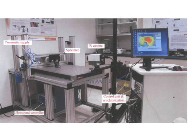
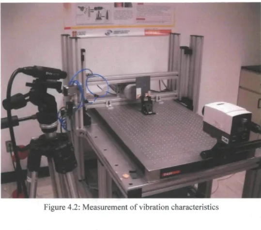
In order to generate mechanical waves, ultrasonic welders Branson 2000b and Branson 2000LPt were used. As a capturing system, Phoenix Indigo IR camera was chosen because of its high performance for NDT applications. Synchronizing signal for acquisition, and input signals for ultrasound generator were generated by the analog output board PCI NI-6711 of National Instruments^ (Figure 4.1). To measure velocity, displacement and frequency of the specimen during the excitation Polytec® laser vibrometer was used (Figure 4.2). All equipment details are available in Appendix.

Figure 4.2: Measurement of vibration characteristics

4.1.1. Acquisition system

To observe the thermal radiation from the specimen surface during experiments, infrared camera Phoenix Indigo produced by FLIR® was used. The focal plane array of this camera contains 640x512 single sensors made of Indium Antimonide (InSb). It operates in the 3 to 5urn spectral range (MWIR) and has a 14-bit dynamic range extension. The noise equivalent temperature difference (NETD) is specified as 25mK.

Moreover, there are other features that make this camera widely used: snapshot (simultaneous) pixel exposure, adjustable gain, variable integration times, high frame rate (up to 22,000 fps) and windowing capability. Camera cooling is made by a Stirling closed cycle cooler that allows keeping the temperature of the FPA around 79K. Specifications are presented in Appendix 1. A set of several infrared lenses Janos Asio is available in the laboratory. Their focal lengths are 13mm, 25mm, 50mm, and 100mm. There are also microscopic lenses of 1 x and 4x magnification.

The camera head is connected to the camera interface, this unit that can be also used to synchronize the camera with an external generated frequency (through analog Syncln and SyncOut ports and a digital Syncln/Out).

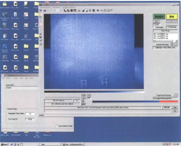
The last essential part of the acquisition system is a personal computer (PC) with a built­in frame grabber. The frame grabber acquires the data streamed from the camera interface towards the PC and stores it in memory. To acquire process, analyze, and the save obtained sequences, the software RTools is installed on the PC (Figure 4.3).

• ­ua1 —

1

I Fit Cwrt 1 H - L M Fit Acqwtd * a*7_*«i_a 2HI_0-5(R__2I>W_4 A M V | « 6 . 1 K [ J k f e j

I 1 " 1 15 F p . T « _ » | q | 15 « • m F p . T « _ » | q | 743S r .>V__oR4M*Er*» r .>V__oR4M*Er*» a»­«l *__l__3 J__i_î__i

Figure 4.3: RTools software

■ i H O 2I1W

RTools allows defining the acquisition settings (e.g. time of acquisition, storage type), display options (e.g. colour palette, display rate) and file name.

4.1.2. Source of ultrasounds

In order to generate low-frequency ultrasonic waves, two sources of ultrasound were used: Branson 2000LPt and Branson 2000b. Despite the fact that they are designed for thermoplastic welding they are well suitable for ultrasound thermography tests.

4.1.3. Branson 2000LPt

Branson 2000LPt is a hand-held ultrasonic welder with a maximum power of 500W. It generates a monofrequent signal (40kHz) with an amplitude between 0 and 100%. To control the source, a special graphical interface was designed by J. M. Piau, the LVSN student working previously with this system (Figure 4.4).

" Ultrason 40 kHz _|n|x|

Excitation i riggei camera Duration |500 ms Min: 1ms M ax: 9000ms Delay |100 m s Min: 100ms M ax: 1000ms go Repeat 17 On go Repeat 17 On Period |1000 m« max: 20000 ms Period |1000 m«

max: 20000 ms Buffer length -| Q00 Buffer length -| Q00 ms

Figure 4.4: Graphique user interface for Branson 2000LPt [33]

Three parameters must be defined for experiment: impulse duration, triggering delay and pulse repetition period. A triggering delay can be used to delay the beginning of ultrasonic signal from the beginning of acquisition; thus, to capture the cold image of the scene (before heating).

4.1.4. Branson 2000b

The operation principle of the ultrasonic source Branson 2000b is the same as of the Branson 2000LPt but it has more options that can be changed. This makes it more effective

in NDT applications. The maximum power of this generator is 2200 W, the frequency range is 15...25kHz. High voltage signal generated by ultrasound generator goes to an ultrasound converter where through the piezoelectric effect, it is converted into mechanical vibrations. To the front side of the converter the titanium hom is attached. Its purpose is to concentrate the energy transferred into the specimen. The integral part of this experimental setup is a pneumatic system of Festoe. It consists of two cylinders, a pressure control unit with gauge

and air dryer, a two-way switch to control the cylinder movement, two adjustable choke valves to control the movement speed, and one choke valve to cool the air towards the converter.

The Branson 2000b can operate in four modes: - burst without frequency modulation, - burst with frequency modulation, - lock-in without frequency modulation, - lock-in with frequency modulation.

First, the main frequency/range of frequencies and the amplitude are set in the software of the Branson UPS (Figure 4.5). Other parameters are next defined in the interface showed in Figure 4.6 (designed by Piau [33]). Using this interface it is possible to generate a simple burst signal (defining amplitude and duration) or burst signals with frequency modulation in the range of 15 to 25kHz (in the form of a ramp or as a periodic function with frequency between 1 and 100Hz) (Figure 4.7). Lock-in (amplitude modulated) signal can be generated defining the shape of the signal (sinusoidal or step), the frequency of modulation, the amplitude and the number of periods. The frequency is variable in the range of 0.1Hz to 10Hz since the duration of the signal is limited to 10 seconds. Lock-in signal can also be frequency modulated (Figure 4.6). As for the Branson 2000LPt, it is possible to program a trigger delay to capture the cold image of the scene.

Fie Password Help

■ l a i x i

Parameter Nane: |DI I fliu I 20KH2, IKP Parameter Index: [1 Connent: |default Seek flnplitude [ I ] - i k p Read HH DIP: i U a r i a n t : |o Held AnpUUnJe \%] Connent: |default

Seek flnplitude [ I ] _{| k i} Read HH DIP: i

U a r i a n t : |o

Held AnpUUnJe \%] _[iu

Seek Ramp Tine [ n s ] _{Jl8 0}

Read HH DIP: i

Held Raup Tine [ u s ] [iu Seek Ramp Tine [ n s ] _{Jl8 0}

Read HH DIP: i

Held Raup Tine [ u s ] lino

Seek Tine [ n s ] _{Jl1 0 8}

Read HH DIP: i

Weld Phase Loop [ ] Ins a Seek Frequ. Hi [• Hz] | | s . o . Read HH DIP: i « e l d Phase Loop Cf [ ] | Ins a Seek Frequ. Hi [• Hz] | | s . o . Read HH DIP: i

« e l d Phase Loop Cf [ ] | lus a Seek Frequ. Lo [«—Hz] ||'. iinn

Read HH DIP: i

Held flnpl. Loop C1 [ | | Hon

Seek Phase Loop [ ] _Jl1"0

Read HH DIP: i

Weld flnpl. loop n? [ ] | la oo Seek Phase Loop CF [ ] ||.00

Read HH DIP: i

Weld L i m i t Hi [*-Hz] | la oo Seek Phase Loop CF [ ] ||.00

Read HH DIP: i

Weld L i m i t Hi [*-Hz] | | ' , 1 ) 1 ! 11

Seek ftnpl. Loop C1 [ ) _{Jl2 8 5}

Read HH DIP: i

Weld L i n i t Lo [*-Hz] | Is unit Seek Rpip]. Loop C2 [ ] _Jl3'°

Read HH DIP: i

Weld Phase L i m i t [ B i t ] | Is unit Seek Rpip]. Loop C2 [ ] _Jl3'°

Read HH DIP: i

Weld Phase L i m i t [ B i t ] | | i «nil

Reserued _II" Read HH DIP: i Weld P h . L i n . T i n e [ n s ] | 160000 Reserued _II8 Read HH DIP: i Resergpd lo Node [ ] JF- SW-DIP Reserued lo

li Frequ. Fixed THzT— *||?I)0I). _{Save ♦ Download} flnpl. Fixed [ I ] |100

F r > q u . Hodul. Loner [Hz F r e q u . Hodul. Upper [Hz

l | | r nun P r i n t | flnpl. Hodul. i MW [%} IS

F r > q u . Hodul. Loner [Hz

F r e q u . _{Hodul. Upper [Hz l||? 0000 E x i t | flnpl. Hodul. Upper [ * ]}

piti

F r > q u . Hodul. Loner [Hz F r e q u . _{Hodul. Upper [Hz l||? 0000}

piti

Ready _{r~r~i /,}

Figure 4.5: Graphical user interface Branson UPS

Ultrasound Vibrothermography Branson 2000b Contrôler Amplitude Frequency modulation P On 9 Ramp C She 5 weep frequency [ Hz Range:! to 100Hz Amplitude Amplitude modulation — W On 0 Sine f" Step Frequency h H 1 00 Hz Range: 0.01 to 10 Hz AmpKudemax I 50 \ Anpitude mil | Ô X W With frequency modulation

| - H 4 Periods

Camera triggw Delay | Ô"

modulating signal

FM

wavefom.

(•) (b) Figure 4.7: Examples of modulating signals and corresponding frequency-modulated

waveforms: a) Ramp modulating signal; b) Periodic modulating signal. [44]

4.1.5. Laser vibrometer

To measure and record the surface velocity and displacement, a single-point laser-Doppler vibrometer (LDV) Polytec was used. LDV operates according to the principles of laser interferometry (Figure 4.8) and the Doppler Effect.

Figure 4.8: Modules of the laser-Doppler vibrometer [45]

A coherent beam generated by an helium neon (HeNe) laser goes to the Beam Splitter 1 where it is divided into two: reference beam and measurement beam. The measurement beam falls on the sample and the light reflected from its surface goes to the Beam Splitter 2. Then this beam travels to the Beam Splitter 3, interfered with the reference beam, and goes to the photodetector. This detector converts this signal into a voltage fluctuation. The

Bragg cell used here is an acousto-optic modulator which purpose is to shift the light frequency by 40MHz to determine the sign of the velocity (if the object moves away or towards interferometer).

The measured frequency shift (Doppler frequency) of the wave is:

2u(t)

ID =—i— cos (a) Equation 4.1 : Doppler frequency

where v(t) is the velocity of the sample, a is the angle between the laser beam and the velocity vector, and A is the wavelength of the emitted wave. Therefore, the output of the photodetector is a frequency modulated signal, with the Bragg cell frequency acting as the carrier frequency, and the Doppler frequency as the modulation frequency.

Using a vibrometer in ultrasound thermography allows defining vibration frequency of the specimen during the test. Examples of velocity vs. time and magnitude vs. frequency graphs are presented in Figure 4.9 and Figure 4.10 respectively.

6­

I

I

I

I

j

j

j

j

j

Figure 4.10: Frequency spectrum

a) Main frequency 20kHz, b) Main frequency 25kHz

sub-harmonics (e.g. 40kHz, 60kHz for 20kHz excitation, 50kHz for 25kHz). Moreover, because of non-linearity of the coupling material, other frequencies occur (acoustic chaos). It was found that their presence enable better defect detectability [15-18].

4.1.6. Coupling and isolation materials

Fixation of the specimen is realized by its clamping between the clamps and the horn with a constant force (usually in the range of 100...150kPa) (Figure 4.11).

Figure 4.11: Specimen clamping

For an efficient ultrasound coupling, tight contact performed through the use of the coupling material. Coupling material should be chosen to match the acoustic impedance of horn (Zh) and specimen (Zs) (Figure 4.12).

horn specimen

Z4

coupling material

Figure 4.12: Scheme of impedances

Since acoustic impedance is defined by the density p and the elastic wave velocity u in the material, acoustic impedance of coupling material can be stated as:

Zc = -JZsZh = J p vs • p.Vh Equation 4.2: Acoustic impedance of coupling material [46]

Another purpose of the coupling materials is to protect the specimen surface from marring that ultrasound horn can produce. As a coupling material, leather, cloth, special coupling liquids, honey and other means can be used. A piece of cloth moistened with water and honey were used in this project. To minimize mechanical energy loss, tips of clamps are made of Teflon and additional insulation material is placed between clamps and specimen. In our case cork was used.

4.2. Ultrasonic testing setup

The setup for ultrasonic testing consists of a bath, a system of axes (X and Y), two controllers (X and Y), two encoders, a flow detector Omniscan MX UT, and a computer with the software that controls the axes.

4.2.1. Water bath

The water bath is a 50cm x 50cm x 30cm plastic bath with a hole in the bottom and a support to hold the specimen. The support includes a 50cm x 48cm x 0,6cm plastic plate with 342 holes of 5mm in diameter. Four aluminum mounts can be fixed on different distances from each other depending on the size of the specimen (Figure 4.13). The bath is filled with water through the hose connected to the tap, and evacuated by the pomp through another hose into the sink.

4.2.2. System of axis XY

The system of axis works in "master to slave" mode (X is "master", Y is "slave"). For axis X positional controller, the encoder has a 159.85 steps/mm resolution. Axis Y moves forward when line X is completed. During the scan the scanner encoders transfer the positional controller coordinates to OmniScan (see next section). The surface dimensions and the resolution programmed in the software of the computer must be the same as those that are entered in OmniScan. There is only one cable connecting the controllers to computer (PS2); thus, the software detects only one controller at a time (Figure 4.14).

4.2.3. Flaw detector OmniScan MX UT

The OmniScan MX UT is an advanced flaw detector from RD Tech (now Olympus NDT) with a module for ultrasonic testing (Figure 4.15). Due to its modular platform, compact size, autonomous power supply, and robust casing, the OmniScan MX is widely used for NDT applications. It can be applied for both manual and automated inspections. Information is displayed on an 8.4-inch real-time monitor with an SVGA resolution of 800 x 600 pixels. To browse through the menu, a scroll knob and function keys can be used (or a mouse and a keyboard externally connected through USB ports). The data can be stored in a Compact Flash card, any USB storage devices, or through network storage.

Chapter 5 Experimental results

This chapter is dedicated to the experimental details, obtained results and their analysis. During this project, tens of experiments were done but only the most significant results are presented in this thesis. In order to compare the performance of different techniques, ultrasonic C-scan testing was performed for some specimens.

The UT tests were carried out with the following acquisition parameters: - integration time - 1.5ms

- window resolution - 640 x 512 pixels - acquisition time - 10-30 sec

- frame rate - 30-50 frames/sec lens - 25mm, 50mm

The legends to the UT images contain the following information:

Configuration (lock-in or burst), main excitation frequency, frequency of amplitude modulation (for lock-in), amplitude, number of periods (for lock-in), duration (for burst), type of image processing.

5.1. CFRP specimens

Mechanical properties of composite materials, such as low weight, robustness, heat resistance, long life expectancy, etc., make them indispensable in aero-space industry. Composites tend to replace other materials in aircraft structures; hence, 25% of Airbus A380 fuselage is made of carbon-fibre reinforced plastics (CFRP), glass-fibre reinforced plastics (GFRP), quartz-fibre reinforced plastic (QFRP), and glass-reinforced fibre metal laminate (GLARE). One of the most probable damages that composite parts could be subject to during assembly, maintenance and exploitation are impacts. The Engineering School of Sao Carlos, University of Sâo Paulo, provided us with CFRP specimens that were previously exposed to impact damages.

5.1.1. Description of specimens and defect production

All specimens have the same dimensions (150 x 100 x 5mm) but different structure.

Specimens #1, #2, #3 and #5 are made of Polyphenylene Sulfide-Carbon (PPS-C) laminate composed of polyphenylene sulfide thermoplastic resin reinforced with T300 JB continuous carbon fibres. The volume fraction of polymer is 50%. Fibre matrix consists of

16 plies following the sequence [(0/90), (+45/-45)2, (0/90)]4. The laminates were hot-compressed at ~300°C.

Specimen #4 is made of Epoxy-Carbon (EPX-C) laminate composed of thermosetting epoxy resin toughened with thermoplastic elastomer particles and reinforced with AGP 193 continuous carbon fibres. The volume fraction of resin in the composite is 60%. The fibre matrix consists of 24 plies following the sequence [(0/90), (+45/-45)2, (0/90)]6. This

laminate was vacuum-bagged in an autoclave at 180°C.

Impact tests were performed in a Charpy pendulum tester with a spherical 16mm steel impactor at an impact rate of 3.5m/s. Specimens #4 and #5 got three impact damages (5, 10 and 20 Joules) each (Figure 5.1).

o»

o «

O 10 J O 10'

O 5J © 5J

USP05 IJSP04 16 plies 24 plies

Figure 5.1 : Specimens #4 and #5

Specimens #1, #2 and #3 were subjected to single impacts of 20, 5 and 10 Joules respectively. Later they were repaired, and no any visible defect occurs now (Figure 5.2).

O

Figure 5.2: Specimens #1, #2, #3 5.1.2. Experiment

The following parameters were employed: excitation frequency

excitation mode

frequency of amplitude modulation nominal amplitude of ultrasound power number of heating periods

position clamping method inspected side pressure isolation material coupling material 15 ... 25 and 40kHz burst, lock-in 0.1 ... 1Hz 0...40% 1 ...9 vertical, horizontal 1, 2 points front, back lOOkPa

cork and Teflon cloth soaked in water