Contents lists available atScienceDirect
Journal of Environmental Management
journal homepage:www.elsevier.com/locate/jenvmanResearch article
Does time since
fire drive live aboveground biomass and stand structure in
low
fire activity boreal forests? Impacts on their management
Jeanne Portier
a,∗, Sylvie Gauthier
b, Guillaume Cyr
c, Yves Bergeron
daDépartement des Sciences Biologiques, Centre for Forest Research, Université du Québec à Montréal, P.O. Box 8888, Stn. Centre-ville, Montréal, QC H3C 3P8, Canada bNatural Resources Canada, Canadian Forest Service, Laurentian Forestry Centre, 1055 du PEPS, P.O. Box 10380, Stn. Sainte-Foy, Québec, QC G1V 4C7, Canada cBureau du forestier en chef, Ministère des Forêts, de la Faune et des Parcs, 845 Boul. St-Joseph, Roberval, QC, G8H 2L6, Canada
dForest Research Institute, Université du Québec en Abitibi-Témiscamingue and Université du Québec à Montréal, 445 Boul. de l'Université, Rouyn-Noranda, QC J9X 5E4,
Canada
A R T I C L E I N F O
Keywords: Boreal forests
Live aboveground biomass Stand structure Time sincefire Lowfire activity Forest management
A B S T R A C T
Boreal forests subject to lowfire activity are complex ecosystems in terms of structure and dynamics. They have a high ecological value as they contain important proportions of old forests that play a crucial role in preserving biodiversity and ecological functions. They also sequester important amounts of carbon at the landscape level. However, the role of time sincefire in controlling the different processes and attributes of those forests is still poorly understood. The Romaine River area experiences afire regime characterized by very rare but large fires and has recently been opened to economic development for energy and timber production. In this study, we aimed to characterize this region in terms of live aboveground biomass, merchantable volume, stand structure and composition, and to establish relations between these attributes and the time since the lastfire. Mean live aboveground biomass and merchantable volume showed values similar to those of commercial boreal coniferous forests. They were both found to increase up to around 150 years after afire before declining. However, no significant relation was found between time since fire and stand structure and composition. Instead, they seemed to mostly depend on stand productivity and non-fire disturbances. At the landscape level, this region contains large amounts of biomass and carbon stored resulting from the longfire cycles it experiences. Although in terms of merchantable volume these forests seemed profitable for the forest industry, a large proportion were old forests or presented structures of old forests. Therefore, if forest management was to be undertaken in this region, particular attention should be given to these old forests in order to protect biodiversity and ecological functions. Partial cutting with variable levels of retention would be an appropriate management strategy as it reproduces the structural complexity of old forests.
1. Introduction
North American boreal forests are shaped by disturbance re-gimes, most particularly wildfires (Brandt, 2009; Johnson, 1992; Payette, 1992). Successional patterns are strongly determined by fires, notably fire intervals and fire severity. With an increasing time since the lastfire, stand biomass and organic layer accumulate for a certain period of time, stand composition changes from mainly shade intolerant species to a higher proportion of shade tolerant species (Paré and Bergeron, 1995; Ward et al., 2014) and stand structure shifts from an even-aged structure to a more irregular one (Bouchard et al., 2008). A stabilization of the aboveground biomass is generally observed between 75 and 90 (Bouchard et al., 2008; Paré and Bergeron, 1995) to 150 years after a fire (Garet et al.,
2009; Gauthier et al., 2010; Harper et al., 2005), depending on the region under study.
In North American boreal forests,fire activity decreases from west to east (Zhang and Chen, 2007). For instance, the North Shore region of Quebec, eastern Canada, experiences fire cycles reaching 785 years (Bouchard et al., 2008; Portier et al., 2016), while they could be as short as 90 years in the Taiga Plain of western Canada (Zhang and Chen, 2007). In the absence offire, stands can become older than the mean longevity of tree species (Boucher et al., 2006; Kneeshaw and Gauthier, 2003). Their dynamics gradually become driven by non-fire disturbances associated with gap dynamics, such as insect outbreaks and windthrows (Blais, 1983; Girard et al., 2014; Pham et al., 2004; Waldron et al., 2013), or simply by senescence mortality. Consequently, such stands are characterized by complex age structures as new cohorts
https://doi.org/10.1016/j.jenvman.2018.07.100
Received 16 April 2018; Received in revised form 27 July 2018; Accepted 29 July 2018
∗Corresponding author.
E-mail address:portier.jeanne@courrier.uqam.ca(J. Portier).
Available online 06 August 2018
0301-4797/ Crown Copyright © 2018 Published by Elsevier Ltd. This is an open access article under the CC BY-NC-ND license (http://creativecommons.org/licenses/BY-NC-ND/4.0/).
establish below older ones (Boucher et al., 2006; De Grandpré et al., 2008).
Over the last few years, the Romaine River region in eastern Quebec has been opened for the forest industry, and close to 280 km2of forests have beenflooded for hydroelectric production. In the context of such economic development, areas experiencing long fire cycles present substantial challenges. First, they contain an important proportion of old forests that are highly complex ecosystems playing a crucial role in preserving biodiversity and ecological functions (Bergeron and Fenton, 2012; Kneeshaw and Gauthier, 2003). Second, boreal forests contain a large share of the global terrestrial carbon pool (Bradshaw and Warkentin, 2015; de Groot et al., 2013; IPCC, 2014). In the context of climate change, the importance of keeping this carbon stored is widely recognized (IPCC, 2014). A large portion of this carbon is released into the atmosphere byfires (Bond-Lamberty et al., 2007; de Groot et al., 2007) but areas subject to lowfire activity can store large amounts at the landscape level (Luyssaert et al., 2008).
Contrary to areas subject to shortfire cycles that are relatively well documented (Harper et al., 2002; Rapanoela et al., 2015), forest attri-butes and dynamics of longfire cycle areas are still poorly known. Yet, live aboveground biomass and merchantable volume, as well as com-position and structure characteristics of such regions would be valuable information for forest managers. Moreover, if forest live aboveground biomass and merchantable volume generally increase with time since the last fire (Harper et al., 2005; Lecomte et al., 2006; Paré and Bergeron, 1995), this relation is still poorly understood in boreal forests subject to long fire cycles. Similarly, the role of fire versus non-fire disturbances in changes in structure and composition of these ecosys-tems needs to be further studied, especially when forest management is involved. Finally, estimating carbon stocks is crucial for a better ap-preciation of the consequences of developing commercial forestry, as well as for simulating alternative scenarios using forestry as a mean to mitigate climate change (e.g. reforestation or intensive management in unproductive sites).
The goal of our study was to characterize the live aboveground biomass, merchantable volume, structure and composition of a fire-scarce region in the Romaine River area of Quebec, Canada, and to establish the relation between these attributes and the time since the lastfire. Our study was based on field inventory data that was also used to extrapolate live aboveground biomass and merchantable volume to the entire study area at the scale of forest stands. Overall, this study intended to improve our understanding of the dynamics of low fire activity areas to help build appropriate forest management strategies in such regions.
2. Material and methods
2.1. Study area
The Romaine River is located in the eastern North Shore region of Quebec, eastern Canada, north of the St. Lawrence River. This region has recently been opened to economic development for hydroelectric energy and forest products (MFFPQ, 2013a). In particular, a portion of the forested landscape has beenflooded permanently to produce elec-tricity. The entire region is mainly characterized by a very low fire activity with rare but largefires. Fire cycles range from ∼200 years in the north to∼8200 years in the south (Gauthier et al., 2015). Our study area is centered on Romaine River and is entirely located within the spruce-moss bioclimatic domain, except for the northernmost portion that lies in the spruce-lichen domain (MFFPQ, 2013b). It covers 72,681 km2and stretches between latitudes 50°N to 53°N, and between longitudes 66°W to 60°W (Fig. 1). This region is the one of the wettest in eastern Canada, with total mean annual precipitation ranging from 754 mm to 1108 mm. Mean annual temperature varies from−4.2 °C to 3.3 °C (means of weather data extracted at the forest-stand level over the 1971–2000 period - Leboeuf et al., 2012). The topography is
variable throughout the study area withflat, sea level areas in the south along the St. Lawrence River, gradually transiting to a highly fractured relief to the north, rising to nearly 1000 m of elevation (Fig. 1). The southern half of the study area mainly sits on bedrocks with very thin mineral soil, while the northern half is largely dominated by thick till deposits. If, as in the rest of the boreal zone of Quebec, black spruce (Picea mariana (Mill.) B.S.P.) is the most represented tree species in the coniferous boreal forests of the North Shore region, longfire cycles and high precipitation make it possible for a significant proportion of balsam fir (Abies balsamea (L.) Mill.) to develop in these forests (Bouchard et al., 2008; De Grandpré et al., 2000). Some other tree species, such as trembling aspen (Populus tremuloides Mich.), white birch (Betula papyrifera Marsh.) and white spruce (Picea glauca (Moench) Voss) can also be found in smaller proportions.
2.2. Field data and basal area calculation
Thefield campaign was conducted in 2014 along a 160-km-long road near Romaine River (Fig. 1). The road was divided into 32 con-secutive 5-km-long by 750-m-wide cells (Portier et al., 2016). In each cell, two points located at a minimum distance of 100 m from the road were randomly generated. These points were used as sampling plots for the estimation of tree basal area (BA) and organic layer thickness. One out of two plots per cell was used for time sincefire estimation. In the northern section of the road, a lower number of plots were sampled because of access issues (total number offield plots = 54). In addition, 164 plots from the Northern Forest Inventory Program (NFIP; 2005 to 2009) of the Ministère des Forêts, de la Faune et des Parcs du Québec (MFFPQ) were added to thefield dataset (Fig. 1). Ourfield protocol was adjusted to match that of the NFIP in order to obtain data of the same kind. Both datasets could therefore be combined without further com-patibility testing. In total, time sincefire data was available for 200 plots: 44field plots (Portier et al., 2016) and 156 inventory plots from the NFIP. Fire history was conventionally reconstructed using den-drochronology. In each stand, the time since the lastfire was inferred from the age of 10 dominant trees (Arno and Sneck, 1977; Johnson and Gutsell, 1994). If this method allows the reconstruction of up to 350 years offire history, time since fire estimates become less precise as they increase (Cyr et al., 2016; Portier et al., 2016). When a stand is older than the oldest tree on-site, assessing a precise stand age becomes impossible. In these cases, a minimum time sincefire was attributed to the stand (Cyr et al., 2016; Portier et al., 2016).
In the 54field plots, BA was assessed per species from the center of the plot using a factor-two wedge prism that selects trees meeting a certain size-distance threshold (Bruce, 1955; Paré et al., 2013). The BA
Fig. 1. Map of study area in the eastern North Shore region of Quebec, Canada, showing the location of sampling sites, elevation profile and bioclimatic do-mains.
of a given species equals two times the number of trees of that species that has been counted with the prism and is expressed in square meters per hectare. In the 164 NFIP inventory plots, BA was calculated from forest stand inventory data. The diameter at breast height (DBH) and height of all trees with a DBH≥ 9 cm were measured in a 400 m2circle. In addition, the DBH of all saplings (3 cm≤ DBH < 9 cm) was mea-sured in a 100 m2circle from the same center. The BA of a tree or sapling in square meters was calculated as:
=
BA π DBH
40 000* ²
tree or sapling (1)
The BA of a given species in square meters per hectare was then defined as:
∑
∑
= +
BAspecies BAtree*25 BAsapling*100 (2)
In order to avoid biases related to the different field methods used (Eastaugh and Hasenauer, 2013), forest stand inventory was also car-ried out in 12field plots (∼25% of the plots) using the same protocol as in the NFIP plots. BA estimates from those 12field plots were compared with the corresponding prism estimates, and a correction was applied to all prism estimates.
2.3. Live aboveground biomass and merchantable volume
Live aboveground biomass was calculated from per species allo-metric equations developed byParé et al. (2013)which estimate the biomass of tree components (stemwood, foliage, branch, and bark) from trees' BA. The biomass of all tree components was summed to obtain the biomass per species in tons per hectare for each plot. Finally, the bio-mass of all species was summed to obtain the total live aboveground biomass of each stand in tons per hectare.
The merchantable volume (i.e. volume in cubic meters per hectare of trees with a DBH≥9 cm –Perron, 2003; Newton, 2012) was cal-culated for each forest inventory plot according to the per species equations developed from DBH and heights of trees (Perron, 2003). As DBH and height were not available where BA was estimated from the wedge prism, the corresponding plots were removed from this calcu-lation (total number of plots in which merchantable volume was cal-culated = 168).
2.4. Composition and structure
Composition was assessed using the proportion of BA of merchan-table trees attributed to black spruce and balsamfir in each plot. Four compositional types were defined: spruce-dominated, spruce-fir, fir-spruce,fir-dominated (Table 1a).
The stand structure of each plot was assessed from the proportion of density and BA of merchantable trees (DBH≥ 9 cm) contained in DBH classes. Plots that did not fall into the four compositional types pre-sented inTable 1a were removed from this analysis. Two-centimeters DBH classes were defined, with “10” being the lowest class and con-taining trees with a DBH between 9 and 11 cm. The few trees presenting a DBH greater than 33 cm were grouped into a“34+” class. In each plot, the reversed cumulative proportions of trees and of BA in each class were calculated to identify groups of similar stand structures. Cumulative proportions were used because they smooth the DBH dis-tributions and thus avoid biases resulting from the use of classes that can lead to important differences between the proportions of two neighboring classes. For instance, consider two plots containing the same number of trees distributed between two DBH classes, but one plot contains all the trees in one class while the other has the trees split equally between the two classes. With a continuous distribution, these two plots would be very similar, while a distribution by class would make them appear completely different.
A k-means clustering method was used to split the plots into homogeneous structure distribution groups (Nlungu-Kweta et al., 2016; Oksanen et al., 2017). The DBH distributions werefirst submitted to a Simple Structure Index (SSI) test using the cascadeKM function of the “vegan” R package (Oksanen et al., 2017). This test divides data into various numbers of clusters based on the distributions provided and produces an SSI value for each number of clusters tested. The highest value indicates the number of clusters into which the data should be divided. Two tofive clusters were tested. Plots were then grouped based on their DBH distributions into the number of clusters obtained with the SSI test using the kmeans function of the“stats” R package.
2.5. Relation between live aboveground biomass, merchantable volume, organic layer thickness, time sincefire, composition and structure
A piecewise regression method was used to determine how long afterfire the live aboveground biomass peaked, and whether this peak was followed by a steady state or a decline (Harper et al., 2005). First, linear regression was used to test the effect of time since fire on bio-mass. Second, a Davies test was performed in order to test for a change of slope and to provide afirst estimate of breakpoint (Muggeo, 2008). Third, a segmented regression was applied using the segmented function of the segmented R package (Muggeo, 2008). The breakpoint estimate returned by the Davies test was used as a starting value to search for the most likely breakpoint. This process was repeated to test the effect of time sincefire on the accumulation of merchantable volume and or-ganic layer thickness.
To test for differences in live aboveground biomass, merchantable volume, time sincefire and organic layer thickness between composi-tional types and structural clusters, one-way ANOVAs followed by Tukey's post-hoc tests were used. In addition, a Chi-square test was conducted between structural clusters and compositional types.
2.6. Extrapolation of live aboveground biomass and merchantable volume to the Romaine River region at the forest stand level
The extrapolation of live aboveground biomass and merchantable volume to the entire study area was done using regression trees. The analysis was carried out at the forest stand level (mean size = 17 ha). Forest stand maps were produced between 2005 and 2008 based on the analysis of Landsat satellite images confirmed with the use of aerial photographs (Leboeuf et al., 2012). Among other attributes, these maps contain information on forest stands' height, density and surficial de-posits. All explanatory variables used in this analysis were compiled at the level of forest stands and are described inTable 2and in the sections below.
Table 1
Description and repartition of compositional types (a). Repartition of structural clusters (b). Only plots corresponding to the four compositional types presented in a) were used in the analyses.
a) Compositional types
Spruce Spruce-Fir Fir-Spruce Fir
Description Percentage relative to the merchantable BA of stands Spruce ≥75% Spruce: 50–75% Fir: Second most represented species Fir: 50–75% Spruce: Second most represented species Fir≥75% Percentage of sites 66.1% 12.8% 10.1% 4.1% b) Structural clusters
Inverted J Intermediate Flat
2.6.1. Rescaling of live aboveground biomass and merchantable volume All plots (field plots and NFIP plots) were assigned to the forest stands in which they fell. Some stands contained two or more plots, in which cases the plots' biomass and merchantable volume were averaged (biomass: six stands containing on average 2.5 plots, mean standard deviation = 5.3; merchantable volume: one stand containing two plots, standard deviation = 1.4). Total live aboveground biomass and mer-chantable volume were split intofive classes based on quantile inter-vals: biomass classes in tons per hectare: 0≤ class 1 < 24.5 ≤ class 2 < 42.5 ≤ class 3 < 54 ≤ class 4 < 71 ≤ class 5 < 188; mer-chantable volume classes in cubic meters per hectare: 0≤ class 1 < 25.5≤ class 2 < 61.5 ≤ class 3 < 96.5 ≤ class 4 < 138 ≤ class 5 < 413.
2.6.2. Forest, soil and topographic data
Classes of stand height and density were reconverted into con-tinuous variables using the median of their classes. Topographic vari-ables were elevation, cosine of aspect, Terrain Ruggedness Index (TRI) and Topographic Position Index (TPI). Topographic variables were averaged using a weighted mean calculation for each forest stand. Surficial deposit drainage was defined based on the dominant surficial deposit of the forest stand and was classified as either xeric, mesic, subhydric, hydric or bare rock when the proportion of mineral soil covering the stand was too small.
2.6.3. Remote sensing spectral data
TERRA MODIS level 1B geolocated top of atmosphere radiance (MOD02) data for summer (July–August) and winter (January–February) 2008 were processed at the Canada Center for Remote Sensing (Pouliot et al., 2009; Trishchenko et al., 2006). They produced orthorectified seasonal mosaics of composite surface flectance at 250-m (Bands 1 and 2) and 500-m (Bands 3 and 6) re-solutions, although different procedures were applied, including the downscaling of the 500-m resolution bands to 250 m (Trishchenko et al., 2006). We used the winter and summer reflectance data in bands 1 (red, 620–670 nm), 2 (near-infrared, 841–876 nm), 3 (blue, 459–479 nm) and 6 (shortwave infrared, 1628–1652 nm) at a 250-m resolution as well as six summer and winter spectral indices that were all derived from summer and winter reflectance data (bands 1, 2 and 3), i.e. Normalized Difference Vegetation Index (NDVI), Wide Dynamic Range Vegetation Index (WDVI), Soil Adjusted Vegetation Index (SAVI), Global Environment Monitoring Index (GEMI), Reduced Simple Ratio (RSR) and Normalized Difference Moisture Index (NDMI) (Pouliot et al., 2009). All spectral bands and indices were extracted for each forest stand using a weighted mean calculation.
2.6.4. Predicted live aboveground biomass and merchantable volume from regression trees
Regression trees are a nonlinear, nonparametric regression method that uses recursive partitioning of the data to model the response variable based on different explanatory variables. Regression trees are made of branches going through different interior nodes (each corre-sponding to one of the explanatory variables) and leading to terminal nodes (values of the response variable) (Breiman et al., 1984; De'ath and Fabricius, 2000). Regression trees of live aboveground biomass and merchantable volume were built using the rpart R package (Therneau et al., 2015). To avoid overfitting, the minimum size of the final nodes for both regression trees was set to 15 observations (between 10 and 15% of the total number of observations).
A k-fold cross-validation was performed on both regression trees by randomly splitting the data set into k mutually exclusive subsets of approximately equal size (Kohavi, 1995). We used k = 10, as it has been suggested to be the most appropriate number of folds for real-world datasets (Kohavi, 1995). One subset was used for validation, while the other nine were used together as a training data set on which a regression tree was built. The cross-validation estimate of accuracy is the proportion of correct classifications in the validation subset. Those steps were repeated ten times so that each subset was used for valida-tion. The mean value of the ten resulting estimates of accuracy provided the overall estimate of accuracy (Kohavi, 1995). This procedure was repeated in a bootstrap process in order to obtain a more precise overall estimate of accuracy, along with the corresponding 95% empirical confidence interval calculated using the lower and upper percentiles. The bootstrap was run using 1000 iterations, after which the confidence interval's width tended to stabilize.
The regression trees were used to predict the live aboveground biomass and merchantable volume of forest stands. For each forest stand, the probabilities of belonging to each class of biomass or mer-chantable volume were extracted from the regression trees. Predicted live aboveground biomass and merchantable volume were then
Table 2
The variables used in the extrapolation of live aboveground biomass and merchantable volume to the study area in the eastern North Shore region of Quebec, Canada, and their description.
Variables Description and range Reference
Forest stands attributes
Height class Classes: 1: > 22 m; 2: 17 to 21 m; 3: 12 to 16 m; 4: 7 to 11 m; 5: 4 to 6 m; 6: 2 to 3 m; 7: < 2 m
(Leboeuf et al., 2012)
Density class Classes: A: > 81%; B: 61 to 81%; C: 41 to 60%; D: 26 to 40%; L: 10 to 25%
Topographic variables
Elevation Range: 1 to 996 m Cosine of aspect Equivalent to the north-south
exposure of a stand. Range: from−1 = facing south to 1 = facing north
TPI Topographic Position Index < 0 tends toward valleys > 0 tends toward hilltops Range: 82 to 90 TRI Terrain Ruggedness Index
Increases with ruggedness of terrain (0 = level) Range: 0 to 138 m Soil variable
Drainage Classes: xeric, mesic, subhydric, hydric or bare rock
(Leboeuf et al., 2012)
MODIS spectral variables
Band 1 (red) Winter and summer surface reflectance bands at 250-m resolution Range B1: 286 to 1398– Range B2: 215 to 3633 Range B3: 867 to 1720– Range B4: 89 to 2370 (Pouliot et al., 2009; Trishchenko et al., 2006) Band 2 (near-infrared) Band 3 (blue) Band 6 (shortwave infrared)
Winter and summer GEMI
Global Environment Monitoring Index
Winter range:−15251 to 5942 Summer range: 1795 to 7809 Winter and summer
NDMI
Normalized Difference Moisture Index
Winter range: 3160 to 9064 Summer range:−3602 to 5566 Winter and summer
NDVI
Normalized Difference Vegetation Index
Winter range:−823 to 4630 Summer range:−1932 to 7709 Winter and summer
RSR
Reduced Simple Ratio Winter range: 424 to 1386 Summer range: 378 to 3263 Winter and summer
SAVI
Soil Adjusted Vegetation Index Winter range:−685 to 292 Summer range:−279 to 5152 Winter and summer
WDVI
Wide Dynamic Range Vegetation Index
Winter range:−7088 to −2942 Summer range:−7618 to 2151
calculated based on the probability and median of each class as:
∑
= ∗
= =
class probability class median
Predicted value class class 1 5 (3) For the whole study area, mean and 95% confidence interval of live aboveground biomass and merchantable volume were calculated using the mean and the lower and upper percentiles of a 1000-iteration bootstrap with replacement of the forest stands. In addition, carbon storage in living trees was estimated using a 0.5 conversion factor from live aboveground biomass (de Groot et al., 2007; Mathews, 1993). Mean predicted live aboveground biomass was also computed for each homogeneousfire zone previously determined based on their fire cycle (Gauthier et al., 2015).
3. Results
Mean live aboveground biomass of all plots was 49.7 t ha−1 (stan-dard deviation = 29.4), while mean merchantable volume was 94.2 m3ha−1(standard deviation = 78.3). The most represented com-positional type was spruce-dominated, followed by spruce-fir, fir-spruce andfinally fir-dominated (Table 1a). The SSI test led to splitting the data into three structural clusters: the“inverted J” structure dominated by small stems; the“intermediate” structure with stems of intermediate DBH; and the“flat” structure presenting a wider range of stem sizes and containing the largest ones (Table 1b,Fig. 2).
3.1. Time sincefire
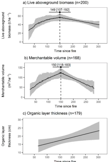
Davies tests performed on linear models of live aboveground bio-mass and time sincefire, as well as of merchantable volume and time since fire were both significant (p-value = 0.013 and 0.004, respec-tively) and both provided a starting breakpoint value at 146 years. Segmented regressions returned a breakpoint at 149 years (95% CI:
107–192) for live aboveground biomass, and at 150 years (95% CI: 118–183) for merchantable volume (Fig. 3a and b). Estimates of all segments were significant (Tables 3a and 3b).
Shaded areas represent 95% confidence intervals. For a) and b), curves and confidence intervals were obtained by bootstrap after 1000 randomizations with replacement of the original dataset and compu-tation of the predicted biomass and merchantable volume values. Mean values were used for the curves, upper and lower percentiles for the confidence intervals. The 95% confidence interval on the time since fire breakpoint estimate is represented by the horizontal black line.
Fig. 2. Relative proportion of merchantable tree density and merchantable BA among DBH classes for each structural cluster.
Fig. 3. Live aboveground biomass (a), merchantable volume (b), and organic layer thickness (c) accumulation with time sincefire.
Table 3
Estimates and p-values (significance level = 0.05) of the segmented regressions of live above ground biomass (a) and merchantable volume (b) and of the linear regression of organic layer thickness (c).
Coefficient p-value a) Live aboveground biomass
Intercept 28.63 6.85 × 10⁻⁴
Time sincefire – segment 1 (< 149 years) 0.20 1.18 × 10⁻² Time sincefire – segment 2 (> 149 years) −0.14 1.28 × 10⁻² b) Merchantable volume
Intercept 30.21 1.22 × 10⁻¹
Time sincefire – segment 1 (< 150 years) 0.64 6.16 × 10⁻³ Time sincefire – segment 2 (> 150 years) −0.62 3.29 × 10⁻³ c) Organic layer thickness
Intercept 11.46 1.88 × 10⁻⁴
The Davies test performed on the linear model of organic layer thickness and time since fire was not significant (p-value = 0.665), suggesting that no breakpoint could be found. Consequently, the seg-mented regression was not performed. Instead, the initial linear model was kept and showed that organic layer thickness significantly in-creased with time sincefire (Table 3c,Fig. 3c).
The ANOVA tests did not show any significant difference between structural clusters and between compositional types in terms of time sincefire (Fig. 4). Nevertheless, the “inverted J” structure tended to have a younger median time sincefire than the other structures (Fig. 5). To better understand why no significant relation was found, mean tree volume was plotted against tree density to visually estimate sites' pro-ductivity (Newton, 2012), according to their time sincefire and struc-tural cluster (Fig. 6). Younger stands with an intermediate or flat structure were mostly productive (high tree density and high mean tree volume), while older stands with an“inverted J” structure were mostly found in unproductive sites.
ANOVA F-tests are shown on the top left corner of each panel along with the significance of the test (* P < 0.05; ** P < 0.01; *** P < 0.001). Tukey's post-hoc tests were used for pairwise comparisons when the ANOVA F-test was significant. Unique letters within each panel reflect significant differences.
3.2. Structure and composition
ANOVAs followed by Tukey's post-hoc tests showed significant dif-ferences in terms of live aboveground biomass and merchantable vo-lume between structural clusters and between compositional types. On the opposite, no significant differences were found in terms of organic
Fig. 4. Mean and standard error of live aboveground biomass, merchantable volume and organic layer thickness for each structural cluster and composi-tional type.
Fig. 5. Time sincefire structure of each structural cluster. Corresponding time sincefire statistics (minimum, 25th percentile, median, 75th percentile and maximum values) are also shown.
Fig. 6. Relation between mean tree volume and tree density of sites according to structural clusters and time sincefire. Site's productivity is maximized where the highest values of both tree volume and tree density are found.
layer thickness (Fig. 4). The Chi-square test showed a significant rela-tion between structural clusters and composirela-tional types (Fig. 7).
3.3. Predicted live aboveground biomass and merchantable volume
The regression trees partitioning forest stands based on their live aboveground biomass and merchantable volume had eight and sevenfinal
nodes, and usedfive and four explanatory variables, respectively (Fig. 8). The 10-fold cross-validation showed an estimate of accuracy of the re-gression trees of live aboveground biomass and merchantable volume of 0.35 (95% CI: 0.30–0.40) and 0.39 (95% CI: 0.34–0.44), respectively.
Fig. 7. Repartition of compositional types into each structural cluster. Chi-square test:χ2= 13.37 (df = 6; p-value = 0.04).
Fig. 8. Regression tree of live aboveground biomass classes (a) and merchan-table volume classes (b).
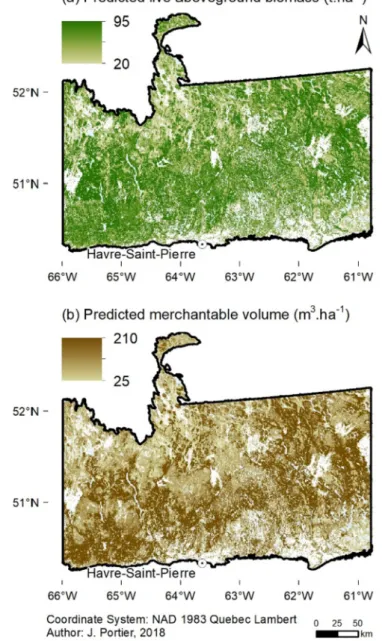
Fig. 9. Map of predicted live aboveground biomass in tons per hectare (a) and predicted merchantable volume in m3per hectare (b). White areas are zones
where no data (explanatory variables) was available.
Fig. 10. Homogeneous fire zones with corresponding fire cycles (FC) over 1972–2009 (Gauthier et al., 2015) and predicted live aboveground biomass (B).
Each interior node constitutes a test with a yes/no answer, from which the“yes” branch goes to the left and the “no” branch goes to the right. Live aboveground biomass classes (t.ha−1): 0≤ class 1 < 24.4≤ class 2 < 42.4 ≤ class 3 < 53.9 ≤ class 4 < 70.8 ≤ class 5 < 188; merchantable volume (m3.ha−1) classes: 0≤ class 1 < 25.4≤ class 2 < 61.3≤ class 3 < 96.5≤ class 4 < 138.1≤ class 5 < 412.7.
Predicted live aboveground biomass and merchantable volume were extracted from the regression trees for all forest stands (Fig. 9). On average, forest stands presented a predicted live aboveground biomass of 58.0 t ha−1 (95% CI: 57.8–58.2) and a merchantable volume of 129.0 m3ha−1 (95% CI: 128.5–129.3). In comparison, live above-ground biomass extracted from Beaudoin et al. (2014) at the forest stand level was 57.0 t ha−1 (95% CI: 56.9–57.1). Predicted live aboveground biomass was higher in areas subject to longerfire cycles (Fig. 10). Furthermore, we estimated from the values of live above-ground biomass that carbon storage in living trees was 29.0 t ha−1 (95% CI: 28.9–29.1).
4. Discussion
4.1. Characterization of forests in a boreal region with lowfire activity Forests in the Romaine River region were dominated by black spruce and, to a lesser extent, by balsamfir. This composition is also prevalent in the western half of the North Shore region of Quebec, east of our study area (Boucher et al., 2006). Stands were split into three structural types– “inverted J”, intermediate and flat – matching those observed by other studies (Boucher et al., 2003; Moussaoui et al., 2016; Nlungu-Kweta et al., 2016). Live aboveground biomass and merchan-table volume significantly increased from the “inverted J” structure to the intermediate structure and finally to the flat structure. The latter presented a wide range of stem sizes, representative of irregular structures characterizing old forests. The complexity of those structures and of the disturbances occurring in such old forests is recognized to be responsible for their high biodiversity of vascular plants, bryophytes, liverworts, lichens (Bergeron and Fenton, 2012), insects (Saint-Germain et al., 2007) and birds (Drapeau et al., 2009), giving them a high ecological value.
We estimated the live aboveground biomass and merchantable volume of the study area to be 58.0 t ha−1(95% CI: 57.8–58.2) and 129.0 m3ha−1 (95% CI: 128.5–129.3), respectively. These values are consistent with larger scale estimates obtained in forested boreal areas, that is, without considering recently burned areas (Beaudoin et al., 2014; Boudreau et al., 2008; Rapanoela et al., 2015). For instance,Boudreau et al. (2008)found that the moderately open coniferous boreal forests of Quebec (density between 26 and 60%) presented an aboveground biomass of 50.2 t ha−1± 1.4 in non-commercial forests and of 58.3 t ha−1± 1.6 in commercial forests. Therefore, forests in the Romaine River area would be mostly akin to commercial boreal forests. However, total predicted aboveground biomass increased between regions experiencing the shortest to the longestfire cycles. At the landscape level, low fire activity areas – mostly covered by forested lands– contain more above- and belowground biomass and thus more carbon stored than regions presenting a large proportion of recently burned areas due to their shorter fire cycles (Gauthier et al., 1996; Luyssaert et al., 2008). In addition, large amounts of carbon are released into the atmosphere byfires burning living and dead biomass in both above- and belowground forest compartments ( Bond-Lamberty et al., 2007; Bradshaw and Warkentin, 2015; de Groot et al., 2007), despite productive young forests partly compensating for these carbon stock losses.
4.2. Biomass accumulation with time sincefire
The pattern of change in live aboveground biomass and merchan-table volume with time sincefire showed an aggradation phase up to
∼150 years, followed by a slow decline. This breakpoint is consistent with thefindings of studies conducted in Quebec (Garet et al., 2009; Gauthier et al., 2010; Harper et al., 2005) and Ontario (Gao et al., 2017). Others found earlier breakpoints in the western North Shore region (∼90 years –Bouchard et al., 2008) and in western Quebec (∼100 years –Harper et al., 2002). Insect outbreaks are the main non-fire disturbance in the North Shore region (MFFP, 2013a; De Grandpré et al., 2008), followed by windthrows (Girard et al., 2014; Waldron et al., 2013). The western North Shore has experienced stronger and more frequent spruce budworm outbreaks than our study area, as well as some hemlock looper outbreaks (MFFP, 2013b; De Grandpré et al., 2008). By inducing high mortality rates and lowering tree growth, these insect disturbances could have turned the aggradation phase's slope into afluctuating pattern (Bouchard et al., 2005).
Decline phases most likely resulted from senescence and non-fire disturbances. First, the mean longevity of canopy trees for black spruce and balsamfir is 100–200 and 60–100 years, respectively (Burns and Honkala, 1990), and balsamfir is shade-tolerant, thus rarely present in thefirst decades after fire (Bouchard et al., 2008; De Grandpré et al., 2000). Second, non-fire disturbances lead to high mortality rates in mature stands (Bouchard et al., 2005; Girard et al., 2014; Pham et al., 2004). However, decline phases often stabilize (Bond-Lamberty et al., 2004; Garet et al., 2009; Harper et al., 2005; Irulappa Pillai Vijayakumar et al., 2016). Although not entirely compensating for the increasing tree mortality with time sincefire, young tree regeneration can allow the upkeep of a certain level of live aboveground biomass and merchantable volume (Garet et al., 2009). Indeed, the decline phase of merchantable volume– that did not consider saplings (DBH < 9 cm) – was steeper than that of live aboveground biomass. In particular cases, as in the Clay Belt area of western Quebec, paludification can lead to a continuous biomass decline by lowering site productivity, regeneration success and tree growth (Lecomte et al., 2006; Simard et al., 2007).
Similarly, when a stand ages, tree mortality leads to the accumu-lation of dead wood that eventually decomposes and thickens the or-ganic layer (Luyssaert et al., 2008; Terrier et al., 2016). However, or-ganic layer thickness in our study area did not reach depths observed in the paludified Clay Belt area. For example, 200 years after fire, the organic layer was approximately 20 cm thick while it could reach 50 cm in the Clay Belt area (Simard et al., 2009, 2007).Ward et al. (2014) concluded that contrary to paludified regions, productivity was not affected by this organic layer accumulation in the North Shore area. Substantial amounts of dead biomass and consequently of carbon are contained in organic layers, which in boreal ecosystems often surpasses live aboveground biomass and carbon (Bradshaw and Warkentin, 2015; Yuan et al., 2008). Old forests are important carbon sinks (Luyssaert et al., 2008) and, therefore, the Romaine River region most likely contains large amounts of carbon stored into its soils.
4.3. Relation between time sincefire and stand structure
One importantfinding of this study is that time since fire did not explain structural nor compositional differences between stands. We demonstrated that instead, stand productivity could be a major driver of stand structure (Boucher et al., 2006; Moussaoui et al., 2016; Newton, 2012). Relatively young stands with aflat structure can be observed when stands are highly productive, as trees can reach large DBHs over a relatively short time. On the contrary, old stands can present an“inverted J” structure when they are located on poor, un-productive sites maintaining a very low tree density regardless of time since the lastfire (Boucher et al., 2006).
As this region experiences longfire cycles (Gauthier et al., 2015; Portier et al., 2016), structural differences could also result from mor-tality caused either by senescence of old stands or by insect outbreaks and/or windthrows (De Grandpré et al., 2000; Girard et al., 2014; Kneeshaw and Gauthier, 2003; Pham et al., 2004). A multi-cohort old stand experiencing gap dynamics driven by small-scale disturbances
would present aflat structure (Kneeshaw and Gauthier, 2003). But if this stand is subjected to strong non-fire disturbances inducing high mortality rates, it could rapidly go back to an“inverted J” structure where large stems would have died and small stems would be new trees regenerating from beneath.
Finally, time sincefire estimates are not always precise, especially when stands are not composed of thefirst post-fire trees (Cyr et al., 2016), which can complicate the determination of relations between time sincefire and composition or structure. Indeed, stands having a time sincefire greater than 150 years are necessarily old, regardless of the precision of the estimate. However, a stand with a small estimated time sincefire would be considered young, even though it could be an old stand that suffered from non-fire disturbances and in which only young trees survived.
4.4. Ecosystem management in a lowfire activity region
Forest management harvests large amounts of biomass and leads to the rejuvenation of forests (Cyr et al., 2009) and to the exportation of important quantities of carbon. On the other hand, the flooding of terrestrial ecosystems for energy production interferes with carbon stocks through two processes, the balance between which is still poorly understood. Flooded biomass eventually releases carbon into the at-mosphere, although this phenomenon can take centuries to millennia in such cold ecosystems (Gennaretti et al., 2014; St. Louis et al., 2000; Teodoru et al., 2012; Tremblay et al., 2004). By no longerfixing carbon, flooded forests also lose their role of carbon sequesters. For these rea-sons, economic development should pay particular attention to the large amounts of highly ecologically valuable old forests and of stored carbon resulting from the longfire cycles. To maintain the proportion of old forests in the landscape, thefirst recommendation for forest man-agement would be to create more protected areas and to apply longer forest rotations in managed forests than those currently used to better match thefire history of the region (Burton et al., 1999; Cyr et al., 2009; Kneeshaw and Gauthier, 2003). In a climate change context, these strategies would also be beneficial as they help maintaining carbon stocks into the forest.
As we showed that in lowfire activity areas, stand productivity and non-fire disturbances might be more important drivers of stand struc-ture than time sincefire, stand structure could constitute a more in-tegrative and complete indicator of the ecosystem's condition than stand age. For this reason, forest management should strengthen the weight of stand structure over stand age in the determination of its strategies. Some ecosystem-based management options are available to preserve old forests or to manage stands so as to maintain or recreate the structural patterns of natural forests (Bauhus et al., 2009; Bergeron et al., 2017; Burton et al., 1999; Shorohova et al., 2011). If clear-cutting should be avoided, partial cutting could be appropriate in structurally complex stands, despite its higher harvesting costs (Bauhus et al., 2009; Bergeron et al., 2017). In particular, some partial cuts treatments maintain a canopy cover by harvesting only large stems and leaving out smaller trees, which helps reproducing the irregular structure of old forests and favors the growth of small stems. As part of ecosystem management objectives, these treatments are recommended in Quebec in regions where pre-industrialfire cycles were long.
In conclusion, our study paints an original and complete picture of lowfire activity boreal forests by establishing relations between forest attributes such as biomass, time sincefire, structure and composition. These forests are highly complex ecosystems driven by processes de-rived from disturbance regimes and stand productivity. If they have a non-negligible commercial potential, they also present a high ecological value because of their large amounts of old forests, biomass and carbon stored. Forest management offers many adapted options and could be implemented on the condition that it accounts for their structural complexity.
Acknowledgements
We are grateful to Alain Leduc (CFR) and Annie Claude Bélisle (UQAT) for valuable methodological advice, and to André Robitaille (MFFP) and David Paré (NRCan) for their ideas on the project. We are grateful to Alain Tremblay (Hydro-Québec) for his helpful advice and his help withfield logistics. We thank Aurélie Terrier, Dave Gervais and Joannie Hébert for their assistance in thefield and Evick Mestre in the laboratory. We also acknowledge the MFFP for providing us with forest inventory andfire archive data. This work was supported by a Natural Sciences and Engineering Research Council of Canada strategic part-nership grant awarded to Y.B. and S.G. and by a Mitacs Accelerate grant awarded to J.P. in partnership with Hydro-Quebec.
References
Arno, S.F., Sneck, K.M., 1977. A Method for Determining Fire History in Coniferous Forests of the Mountain West.
Bauhus, J., Puettmann, K., Messier, C., 2009. Silviculture for old-growth attributes. For. Ecol. Manag. 258, 525–537.https://doi.org/10.1016/j.foreco.2009.01.053. Beaudoin, A., Bernier, P.Y., Guindon, L., Villemaire, P., Guo, X.J., Stinson, G., Bergeron,
T., Magnussen, S., Hall, R.J., 2014. Mapping attributes of Canada's forests at mod-erate resolution through kNN and MODIS imagery. Can. J. For. Res. 44, 521–532.
https://doi.org/10.1139/cjfr-2013-0401.
Bergeron, Y., Fenton, N.J., 2012. Boreal forests of eastern Canada revisited: old growth, nonfire disturbances, forest succession, and biodiversity. Botany 90, 509–523.
https://doi.org/10.1139/B2012-034.
Bergeron, Y., Irulappa Pillai Vijayakumar, D.B., Ouzennou, H., Raulier, F., Leduc, A., Gauthier, S., 2017. Projections of future forest age class structure under the influence offire and harvesting: implications for forest management in the boreal forest of eastern Canada. For. Int. J. For. Res. 90, 485–495.https://doi.org/10.1093/forestry/ cpx022 Projections.
Blais, J.R., 1983. Trends in the frequency, extent, and severity of spruce budworm out-breaks in eastern Canada. Can. J. For. Res. 13, 539–547.
Bond-Lamberty, B., Peckham, S.D., Ahl, D.E., Gower, S.T., 2007. Fire as the dominant driver of central Canadian boreal forest carbon balance. Nature 450, 89–92.https:// doi.org/10.1038/nature06272.
Bond-Lamberty, B., Wang, C., Gower, S.T., 2004. Net primary production and net eco-system production of a boreal black spruce wildfire chronosequence. Glob. Change Biol. 10, 473–487.https://doi.org/10.1111/j.1529-8817.2003.0742.x.
Bouchard, M., Kneeshaw, D., Bergeron, Y., 2005. Mortality and stand renewal patterns following the last spruce budworm outbreak in mixed forests of western Quebec. For. Ecol. Manag. 204, 297–313.https://doi.org/10.1016/j.foreco.2004.09.017. Bouchard, M., Pothier, D., Gauthier, S., 2008. Fire return intervals and tree species
suc-cession in the North Shore region of eastern Quebec. Can. J. For. Res. 38, 1621–1633.
https://doi.org/10.1139/X07-201.
Boucher, D., De Grandpré, L., Gauthier, S., 2003. Développement d'un outil de classifi-cation de la structure des peuplements et comparaison de deux territoires de la pessiere à mousses du Québec. For. Chron. 79, 318–328.
Boucher, D., Gauthier, S., De Grandpré, L., 2006. Structural changes in coniferous stands along a chronosequence and a productivity gradient in the northeastern boreal forest of Québec. Ecoscience 13, 172–180. https://doi.org/10.2980/i1195-6860-13-2-172.1.
Boudreau, J., Nelson, R.F., Margolis, H.A., Beaudoin, A., Guindon, L., Kimes, D.S., 2008. Regional aboveground forest biomass using airborne and spaceborne LiDAR in Québec. Remote Sens. Environ. 112, 3876–3890.https://doi.org/10.1016/j.rse. 2008.06.003.
Bradshaw, C.J.A., Warkentin, I.G., 2015. Global estimates of boreal forest carbon stocks andflux. Glob. Planet. Change 128, 24–30.https://doi.org/10.1016/j.gloplacha. 2015.02.004.
Brandt, J.P., 2009. The extent of the North American boreal zone. Environ. Rev. 17, 101–161.https://doi.org/10.1139/A09-004.
Breiman, L., Friedman, J., Stone, C.J., Olshen, R.A., 1984. Classification and Regression Trees. CRC Press, Boca Raton, FL.
Bruce, D., 1955. A new way to look at trees. J. For. 53, 163–167.
Burns, R.M., Honkala, B.H., 1990. In: Silvics of North America. Volume 1: Conifers, Agriculture Handbook 654 USDA Forest Service, Washington, DC.
Burton, P.J., Kneeshaw, D.D., Coates, K.D., 1999. Managing forest harvesting to maintain old growth in boreal and sub-boreal forests. For. Chron. 75, 623–631.https://doi. org/10.5558/tfc75623-4.
Cyr, D., Gauthier, S., Bergeron, Y., Carcaillet, C., 2009. Forest management is driving the eastern North American boreal forest outside its natural range of variability. Front. Ecol. Environ. 7, 519–524.https://doi.org/10.1890/080088.
Cyr, D., Gauthier, S., Boulanger, Y., Bergeron, Y., 2016. Quantifyingfire cycle from dendroecological records using survival analyses. Forests 7, 1–21.https://doi.org/10. 3390/f7070131.
De'ath, G., Fabricius, K.E., 2000. Classification and regression trees: a powerful yet simple technique for ecological data analysis. Ecology 81, 3178–3192.https://doi.org/10. 2307/177409.
De Grandpré, L., Gauthier, S., Allain, C., Cyr, D., Périgon, S., Thu Phan, A., Boucher, D., Morissette, J., Reyes, G., Aakala, T., Kuuluvainen, T., 2008. Vers un aménagement écosystémique de la forêt boréale de la Côte Nord. In: Aménagement Écosystémique En Forêt Boréale. Les Presses de l'Université du Québec, Québec, QC, Canada, pp. 241–268.
De Grandpré, L., Morisette, J., Gauthier, S., 2000. Long-term post-fire changes in the northeastern boreal forest of Quebec. J. Veg. Sci. 11, 791–800.
de Groot, W.J., Cantin, A.S., Flannigan, M.D., Soja, A.J., Gowman, L.M., Newbery, A., 2013. A comparison of Canadian and Russian boreal forestfire regimes. For. Ecol. Manage 294, 23–34.https://doi.org/10.1016/j.foreco.2012.07.033.
de Groot, W.J., Landry, R., Kurz, W.A., Anderson, K.R., Englefield, P., Fraser, R.H., Hall, R.J., Banfield, E., Raymond, D.A., Decker, V., Lynham, T.J., Pritchard, J.M., 2007. Estimating direct carbon emissions from Canadian wildlandfires. Int. J. Wildl. Fire 16, 593–606.https://doi.org/10.1071/WF06150.
Drapeau, P., Nappi, A., Imbeau, L., Saint-Germain, M., 2009. Standing deadwood for keystone bird species in the eastern boreal forest: managing for snag dynamics. For. Chron. 85, 227–234.
Eastaugh, C.S., Hasenauer, H., 2013. Biases in volume increment estimates derived from successive angle count sampling. For. Sci. 59, 1–14.https://doi.org/10.5849/forsci. 11-007.
Gao, B., Taylor, A.R., Searle, E.B., Kumar, P., Ma, Z., Hume, A.M., Chen, H.Y.H., 2017. Carbon storage declines in old boreal forests irrespective of succession pathway. Ecosystems.https://doi.org/10.1007/s10021-017-0210-4.
Garet, J., Pothier, D., Bouchard, M., 2009. Predicting the long-term yield trajectory of black spruce stands using time sincefire. For. Ecol. Manag. 257, 2189–2197.https:// doi.org/10.1016/j.foreco.2009.03.001.
Gauthier, S., Boucher, D., Morissette, J., De Grandpré, L., 2010. Fifty-seven years of composition change in the eastern boreal forest of Canada. J. Veg. Sci. 21, 772–785.
https://doi.org/10.1111/j.1654-1103.2010.01186.x.
Gauthier, S., Leduc, A., Bergeron, Y., 1996. Forest dynamics modelling under naturalfire cycles: a tool to define natural mosaic diversity for forest management. Environ. Monit. Assess. 39, 417–434.
Gauthier, S., Raulier, F., Ouzennou, H., Saucier, J., 2015. Strategic analysis of forest vulnerability to risk related tofire: an example from the coniferous boreal forest of Quebec. Can. J. For. Res. 45, 553–565.https://doi.org/10.1139/cjfr-2014-0125. Gennaretti, F., Arseneault, D., Bégin, Y., 2014. Millennial stocks andfluxes of large woody
debris in lakes of the North American taiga. J. Ecol. 102, 367–380.https://doi.org/ 10.1111/1365-2745.12198.
Girard, F., De Grandpre, L., Ruel, J.C., 2014. Partial windthrow as a driving process of forest dynamics in old-growth boreal forests. Can. J. For. Res. 44, 1165–1176.
https://doi.org/10.1139/cjfr-2013-0224.
Harper, K.A., Bergeron, Y., Drapeau, P., Gauthier, S., De Grandpré, L., 2005. Structural development followingfire in black spruce boreal forest. For. Ecol. Manag. 206, 293–306.https://doi.org/10.1016/j.foreco.2004.11.008.
Harper, K.A., Bergeron, Y., Gauthier, S., Drapeau, P., 2002. Post-fire development of canopy structure and composition in black spruce forests of Abitibi, Québec: a landscape scale study. Silva Fenn. 36, 249–263.
IPCC, 2014. Climate Change 2014: Synthesis Report. Contribution of Working Groups I, II and III to the Fifth Assessment Report of the Intergovernmental Panel on Climate Change. IPCC, Geneva, Switzerland.
Irulappa Pillai Vijayakumar, D.B., Raulier, F., Bernier, P., Paré, D., Gauthier, S., Bergeron, Y., Pothier, D., 2016. Cover density recovery afterfire disturbance controls landscape aboveground biomass carbon in the boreal forest of eastern Canada. For. Ecol. Manag. 360, 170–180.https://doi.org/10.1016/j.foreco.2015.10.035.
Johnson, E.A., 1992. Fire and Vegetation Dynamics - Studies from the North American Boreal Forest. Cambridge University Press, Cambridge, UK.https://doi.org/10.1046/ j.1469-8137.1997.00703-3.x.
Johnson, E.A., Gutsell, S.L., 1994. Fire frequency models, methods and interpretations. Adv. Ecol. Res. 25, 239–287.
Kneeshaw, D., Gauthier, S., 2003. Old growth in the boreal forest: a dynamic perspective at the stand and landscape level. Environ. Rev. 11, 99–114.https://doi.org/10.1139/ A03-010.
Kohavi, R., 1995. A study of cross-validation and bootstrap for accuracy estimation and model selection. In: International Joint Conference on Artificial Intelligence. Morgan Kaufmann Publishers, San Francisco, pp. 1137–1145.https://doi.org/10.1067/mod. 2000.109031.
Leboeuf, A., Robitaille, A., Létourneau, J.-P., Morneau, C., Bourque, L., 2012. Norme de cartographie écoforestière du programme d'inventaire écoforestier nordique (PIEN). Ministère des Ressources naturelles, Secteur des forêts, Québec, QC, Canada. Lecomte, N., Simard, M., Fenton, N., Bergeron, Y., 2006. Fire severity and long-term
ecosystem biomass dynamics in coniferous boreal forests of eastern Canada. Ecosystems 9, 1215–1230.https://doi.org/10.1007/s10021-004-0168-x. Luyssaert, S., Schulze, E.-D., Börner, A., Knohl, A., Hessenmöller, D., Law, B.E., Ciais, P.,
Grace, J., 2008. Old-growth forests as global carbon sinks. Nature 455, 213–215.
https://doi.org/10.1038/nature07276.
Mathews, G., 1993. The Carbon Content of Trees. Forestry Commission Technical Paper 4. Edinburgh, Scotland.
MFFPQ, 2013a. Rapport du Comité scientifique chargé d'examiner la limite nordique des forêts attribuables. Québec, QC, Canada.
MFFPQ, 2013b. Cartographie numérique des niveaux supérieurs du Système hiérarchique de classification écologique et banque de données descriptives des districts écologiques. Québec, QC, Canada.
Moussaoui, L., Fenton, N.J., Leduc, A., Bergeron, Y., 2016. Can retention harvest maintain natural structural complexity? A comparison of post-harvest and post-fire residual patches in boreal forest. Forests 7, 1–17.https://doi.org/10.3390/f7100243. Muggeo, V.M.R., 2008. segmented: an R package tofit regression models with broken-line
relationships. R. News 8, 20–25.https://doi.org/10.1159/000323281. Newton, P.F., 2012. A decision-support system for forest density management within
upland black spruce stand-types. Environ. Model. Software 35, 171–187.https://doi. org/10.1016/j.envsoft.2012.02.019.
Nlungu-Kweta, P., Leduc, A., Bergeron, Y., 2016. Climate and disturbance regime effects on aspen (Populus tremuloides Michx.) stand structure and composition along an east–west transect in Canada's boreal forest. Forestry 90, 70–81.https://doi.org/10. 1093/forestry/cpw026.
Oksanen, J.F., Blanchet, G., Friendly, M., Kindt, R., Legendre, P., McGlinn, D., Minchin, P.R., O'Hara, R.B., Simpson, Gavin L., Solymos, Peter, Stevens, M. Henry H., E.S, Wagne, H., 2017. Package“vegan”. [WWW Document]. URL.https://cran.r-project. org/web/packages/vegan/vegan.pdf, Accessed date: 23 March 2017.
Paré, D., Bergeron, Y., 1995. Above-ground biomass accumulation along a 230-year chronosequence in the southern portion of the Canadian boreal forest. J. Ecol. 83, 1001–1007.https://doi.org/10.2307/2261181.
Paré, D., Bernier, P., Lafleur, B., Titus, B.D., Thiffault, E., Maynard, D.G., Guo, X., 2013. Estimating stand-scale biomass, nutrient contents, and associated uncertainties for tree species of Canadian forests. Can. J. For. Res. 43, 599–608.https://doi.org/10. 1139/cjfr-2012-0454.
Payette, S., 1992. Fire as a controlling process in the North American boreal forest. In: Shugart, H.H., Leemans, R., Bonan, G.B. (Eds.), A System Analysis of the Global Boreal Forest. Cambridge University Press, Cambridge, UK, pp. 144–169.https://doi. org/10.1017/CBO9780511565489.006.
Perron, J.-Y., 2003. Tarif de cubage général - volume marchand brut, 3e édition. Ministère des Ressources naturelles, de la Faune et des Parcs, Direction des in-ventaires forestiers, Québec, QC, Canada.
Pham, A.T., De Grandpré, L., Gauthier, S., Bergeron, Y., 2004. Gap dynamics and re-placement patterns in gaps of the northeastern boreal forest of Quebec. Can. J. For. Res. 34, 353–364.https://doi.org/10.1139/x03-265.
Portier, J., Gauthier, S., Leduc, A., Arseneault, D., Bergeron, Y., 2016. Fire regime along latitudinal gradients of continuous to discontinuous coniferous boreal forests in eastern Canada. Forests 7, 211.https://doi.org/10.3390/f7100211.
Pouliot, D., Latifovic, R., Fernandes, R., Olthof, I., 2009. Evaluation of annual forest disturbance monitoring using a static decision tree approach and 250 m MODIS data. Remote Sens. Environ. 113, 1749–1759.https://doi.org/10.1016/j.rse.2009.04.008. Rapanoela, R., Raulier, F., Gauthier, S., Ouzennou, H., Saucier, J., Bergeron, Y., 2015.
Contrasting current and potential productivity and the influence of fire and species composition in the boreal forest: a case study in eastern Canada. Can. J. For. Res. 45, 541–555.https://doi.org/10.1139/cjfr-2014-0124.
Saint-Germain, M., Drapeau, P., Buddle, C.M., 2007. Host-use patterns of saproxylic phloeophagous and xylophagous Coleoptera adults and larvae along the decay gra-dient in standing dead black spruce and aspen. Ecography (Cop.) 30, 737–748.
https://doi.org/10.1111/j.2007.0906-7590.05080.x.
Shorohova, E., Kneeshaw, D., Kuuluvainen, T., Gauthier, S., 2011. Variability and dy-namics of old-growth forests in the circumboreal zone: implications for conservation, restoration and management. Silva Fenn. 45, 785–806.
Simard, M., Bernier, P.Y., Bergeron, Y., Paré, D., Guérine, L., 2009. Paludification dy-namics in the boreal forest of the James Bay Lowlands: effect of time since fire and topography. Can. J. For. Res. 39, 546–552.https://doi.org/10.1139/X08-195.
Simard, M., Lecomte, N., Bergeron, Y., Bernier, P.Y., Paré, D., 2007. Forest productivity decline caused by successional paludification of boreal soils. Ecol. Appl. 17, 1619–1637.
St. Louis, V.L., Kelly, C.A., Duchemin, E., Rudd, J.W.M., Rosenberg, D.M., 2000. Reservoir surfaces as sources of greenhouse gases to the atmosphere: a global estimate. Bioscience 50, 766–775.
Teodoru, C.R., Bastien, J., Bonneville, M.-C., del Giorgio, P.A., Demarty, M., Garneau, M., Hélie, J.-F., Pelletier, L., Prairie, Y.T., Roulet, N.T., Strachan, I.B., Tremblay, A., 2012. The net carbon footprint of a newly created boreal hydroelectric reservoir. Global Biogeochem. Cycles 26, 1–14.https://doi.org/10.1029/2011GB004187.
Terrier, A., Paquette, M., Gauthier, S., Girardin, M.P., Pelletier-Bergeron, S., Bergeron, Y., 2016. Influence of fuel load dynamics on carbon emission by wildfires in the Clay Belt boreal landscape. Forests 8, 1–20.https://doi.org/10.3390/F8010009.
Therneau, T., Atkinson, B., Ripley, B., 2015. Package“rpart. [WWW Document]. URL.
http://cran.r-project.org/web/packages/rpart/rpart.pdf, Accessed date: 1 January 2017.
Tremblay, A., Lambert, M., Gagnon, L., 2004. Do hydroelectric reservoirs emit green-house gases? Environ. Manag. 33, 509–517. https://doi.org/10.1007/s00267-003-9158-6.
Trishchenko, A.P., Luo, Y., Khlopenkov, K.V., 2006. A method for downscaling MODIS land channels to 250 m spatial resolution using adaptive regression and normal-ization. In: Ehlers, M., Michel, U. (Eds.), SPIE Proceedings Vol. 6366: Remote Sensing for Environmental Monitoring, GIS Applications, and Geology VI. International Society for Optics and Photonics, Ottawa, ON, Canada, 636607.https://doi.org/10. 1117/12.689157.
Waldron, K., Ruel, J.-C., Gauthier, S., 2013. Forest structural attributes after windthrow and consequences of salvage logging. For. Ecol. Manag. 289, 28–37.https://doi.org/ 10.1016/j.foreco.2012.10.006.
Ward, C., Pothier, D., Paré, D., 2014. Do boreal forests needfire disturbance to maintain productivity? Ecosystems 17, 1053–1067. https://doi.org/10.1007/s10021-014-9782-4.
Yuan, F., Arain, M.A., Barr, A.G., Black, T.A., Bourque, C.P.-A., Coursolle, C., Margolis, H.A., McCaughey, J.H., Wofsy, S.C., 2008. Modeling analysis of primary controls on net ecosystem productivity of seven boreal and temperate coniferous forests across a continental transect. Glob. Change Biol. 14, 1765–1784.https://doi.org/10.1111/j. 1365-2486.2008.01612.x.
Zhang, Q., Chen, W., 2007. Fire cycle of the Canada's boreal region and its potential response to global change. J. For. Res. 18, 55–61. https://doi.org/10.1007/s11676-007-0010-3.