Are Children Decision-Makers Within the Household?

Texte intégral

(1)2010s-17. Are Children Decision-Makers Within the Household? Anyck Dauphin, Abdel-Rahmen El Lahga, Bernard Fortin, Guy Lacroix. Série Scientifique Scientific Series. Montréal Avril 2010. © 2010 Anyck Dauphin, Abdel-Rahmen El Lahga, Bernard Fortin, Guy Lacroix. Tous droits réservés. All rights reserved. Reproduction partielle permise avec citation du document source, incluant la notice ©. Short sections may be quoted without explicit permission, if full credit, including © notice, is given to the source..

(2) CIRANO Le CIRANO est un organisme sans but lucratif constitué en vertu de la Loi des compagnies du Québec. Le financement de son infrastructure et de ses activités de recherche provient des cotisations de ses organisations-membres, d’une subvention d’infrastructure du Ministère du Développement économique et régional et de la Recherche, de même que des subventions et mandats obtenus par ses équipes de recherche. CIRANO is a private non-profit organization incorporated under the Québec Companies Act. Its infrastructure and research activities are funded through fees paid by member organizations, an infrastructure grant from the Ministère du Développement économique et régional et de la Recherche, and grants and research mandates obtained by its research teams. Les partenaires du CIRANO Partenaire majeur Ministère du Développement économique, de l’Innovation et de l’Exportation Partenaires corporatifs Banque de développement du Canada Banque du Canada Banque Laurentienne du Canada Banque Nationale du Canada Banque Royale du Canada Banque Scotia Bell Canada BMO Groupe financier Caisse de dépôt et placement du Québec Fédération des caisses Desjardins du Québec Gaz Métro Hydro-Québec Industrie Canada Investissements PSP Ministère des Finances du Québec Power Corporation du Canada Raymond Chabot Grant Thornton Rio Tinto State Street Global Advisors Transat A.T. Ville de Montréal Partenaires universitaires École Polytechnique de Montréal HEC Montréal McGill University Université Concordia Université de Montréal Université de Sherbrooke Université du Québec Université du Québec à Montréal Université Laval Le CIRANO collabore avec de nombreux centres et chaires de recherche universitaires dont on peut consulter la liste sur son site web. Les cahiers de la série scientifique (CS) visent à rendre accessibles des résultats de recherche effectuée au CIRANO afin de susciter échanges et commentaires. Ces cahiers sont écrits dans le style des publications scientifiques. Les idées et les opinions émises sont sous l’unique responsabilité des auteurs et ne représentent pas nécessairement les positions du CIRANO ou de ses partenaires. This paper presents research carried out at CIRANO and aims at encouraging discussion and comment. The observations and viewpoints expressed are the sole responsibility of the authors. They do not necessarily represent positions of CIRANO or its partners.. ISSN 1198-8177. Partenaire financier.

(3) Are Children Decision-Makers Within the Household?* Anyck Dauphin†, Abdel-Rahmen El Lahga‡, Bernard Fortin§ Guy Lacroix ** Résumé Les enfants sont rarement pris en considération dans les modèles de comportement des ménages. On présume généralement qu’ils ne possèdent ni la capacité ni le pouvoir d’influencer le processus décisionnel du ménage. La littérature portant sur les modèles collectifs a, jusqu’à maintenant, intégré les enfants par le truchement des « préférences altruistes » de leurs parents [Bourguignon (1999)] ou les a traités comme des biens publics des ménages [Blundell et al. (2005)]. Le présent document tente de déterminer si les enfants d’un certain âge jouent un rôle décisionnel. Nous mettons l’accent sur le processus de prise de décision au sein des ménages composés de deux adultes et d’un enfant âgé d’au moins 16 ans vivant ensemble. Nous résumons d’abord les principales restrictions qui ont été proposées pour tester le modèle collectif dans le contexte de décideurs multiples [Chiappori et Ekeland (2006)]. Nous montrons aussi que les contraintes paramétriques laissent supposer un nombre minimal de décideurs. Ensuite, nous appliquons ces tests aux données extraites d’une série de sondages sur les dépenses des familles au Royaume-Uni. Nos résultats fournissent l’évidence que les enfants âgés de 16 ans et plus vivant avec leurs parents influencent le processus décisionnel du ménage. Lorsque l’analyse est stratifiée selon l’âge et le genre, nos résultats révèlent qu’il en est de même pour les enfants âgés entre 16 et 21 ans, filles ou garçons. Le modèle collectif n’est jamais rejeté. Mots clés : allocation intra-ménage, modèles collectifs de ménages, enfants, analyse de la demande, efficacité parétienne, tests de classement.. *. We are grateful to the Central Statistical Office for granting us access to the British Family Expenditure Survey. We also wish to thank the Centre Interuniversitaire sur le Risque, les Politiques Économiques et l’Emploi (CIRPÉE), the Canada Chair of Research in the Economics of Social Policies and Human Resources, and the Consejo Superior de Investigacion Cientifico de España for their financial assistance. This article was partly written while Lacroix was a visiting professor at the Institut de Anàlisi Econòmica in Barcelona and while Fortin was a visiting researcher at the Université de Paris 1 Panthon-Sorbonne. We are also indebted to Eugene Choo, Olivier Donni, Nicolas Jacquemet, Costas Meghir, Steve Pischke, Arthur van Soest, and two anonymous referees for their detailed and informative comments on an initial version. We also benefited from useful discussions with Georges Bresson, Martin Browning, Pierre-André Chiappori, Hélène Couprie, Frank Kleibergen, Chris Flinn, Jean-Marc Robin, and Frances Woolley. † Université du Québec en Outaouais; anyck.dauphin@uqo.ca. ‡ Institut Supérieur de Gestion de Tunis, Tunisia, and U.A.QU.AP.; abdelrahmen.ellahga@gnet.tn. § Département d’économique, Université Laval, CIRPÉE, CIRANO; bernard.fortin@ecn.ulaval.ca. ** Département d'Economique, Pavillon J.A. De Sève, Québec, Québec, G1K 7P4, Canada. Tél : 418-656-5122. Fax : 418-656-2707. E-mail : Guy.Lacroix@ecn.ulaval.ca..

(4) Abstract. Children are seldom accounted for in household behavioural models. They are usually assumed to have neither the capacity nor the power to influence the household decision process. The literature on collective models has so far incorporated children through the “caring preferences” of their parents [Bourguignon (1999)] or has treated them as household public goods [Blundell et al. (2005)]. This paper seeks to determine whether children of a certain age are decision-makers. We focus on the decision-making process within households composed of two adults and one child of at least 16 years of age living together. We first summarise the main restrictions that have been proposed to test the collective model in the context of multiple decision-makers [Chiappori and Ekeland (2006)]. We also show how a minimal number of decision-makers can be inferred from parametric constraints. Second, we apply these tests on data drawn from a series of U.K. Family Expenditure Surveys. Our results show clear evidence that children aged 16 and more and living with their parents influence the household decision-making process. When the analysis is stratified by age and by gender, our results reveal that it is also the case for children aged between 16 and 21 and for daughters. The collective model is never rejected. Keywords: intra-household allocation, collective household models, children, demand analysis, Pareto efficiency, rank tests. Codes JEL : D11, D12, D79, J13.

(5) 1. Introduction. Children are seldom accounted for in household behavioural models. At best, they are considered bystanders assumed not to have the capacity nor the power to influence the household decision process. This is not really surprising since until recently households were assumed to act as if their members maximised a unique utility function under the household budget constraint. This so-called unitary model has been forcefully challenged in the last two decades both on theoretical and empirical grounds. At the theoretical level, the unitary model has been challenged for its failure to acknowledge methodological individualism, which is a fundamental tenet of microeconomic theory. Because “it is necessary to base all accounts of economic interaction on individual behaviour” [Arrow (1994)], each member’s preferences should indeed be explicitly taken into account. At the empirical level, the restrictions of the unitary model have been widely tested and generally rejected [e.g., Fortin and Lacroix (1997); Alderman et al. (1997); Cherchye et al. (2009)]. The collective household model has been proposed partly in response to the dissatisfaction with the unitary model. The former simply assumes that the family decision process, whatever its exact nature, leads to Pareto efficient outcomes. One interesting feature of the collective model is that it does not require the specification of the bargaining process. Evidently, the generality of the efficiency assumption comes at a price: the model is not very informative about which variables, other than those in the budget constraint, may influence the decision process. In particular, the model is totally silent as to the role children may play in the process. The literature on the collective model has so far incorporated children through the “caring preferences” of their parents [Bourguignon (1999)] or has treated them as household public goods [Blundell et al. (2005)].1 Yet every parent knows that children, even at a very early age, have their own preferences over consumption and their parents’ labour supply. In an experiment, Harbaugh et al. (2001) found that “at age 7 children’s choices about consumption goods show clear evidence of rationality, though also many inconsistencies. By age 11, choices by children [...] are as rational as choices by adults”. Harbaugh et al. (2003) further showed in another experiment that children display good bargaining skills as early as 7 years of age. Naturally, one may object to the inclusion of young children as decision-makers on several grounds. Within a bargaining framework, the child’s threat point could correspond to his level of well-being in a non-cooperating equilibrium with his parents. Parents could then resort to punishment to reduce their child’s bargaining power or to make it non existent.2 One could also argue that the bargaining power of young children is so low and their preferences “defined” over such a limited subset of goods that it is pointless to treat them as economic agents. Yet the relevance of modelling the decision power of older children cannot be discarded so easily. As children grow up, they gradually become more autonomous. Their autonomy eventually leads to the possibility of earning income and, later on, of becoming fully independent at the legal age of majority. Therefore the well-being that 1. A number of papers in the bargaining literature have explicitly accounted for children’s preferences, although the proposed models were not meant to analyse household consumption or labour supply decisions. For instance, Burton et al. (2002) propose a principalagent model between the parents and the child to study the interaction between parenting style and child conduct. Lundberg et al. (2007) develop a non-cooperative model of parenting control over child behaviour. The model incorporates child resistance and seeks to examine the determinants of decision-making power by children and adolescents. Finally, Hao et al. (2008) present a two-stage repeated game in which the children decide whether to drop out of school or teenage daughters decide whether to give birth. Parents must then decide whether or not to provide support to their children beyond the age of 18. 2 Conditional positive transfers made by a parent to his child may also induce the latter to behave as if there were only one decisionmaker within the household. However, this Beckerian rotten kid theorem [Becker (1974)] requires many restrictive assumptions to hold [e.g., Bergstrom (1989)].. 1.

(6) a child can attain in a non-cooperative equilibrium might improve as he grows up and so should his bargaining position. Whether and at which age children should be considered as economic agents in household consumption and labour decisions is thus an empirical issue. Conceiving family decisions as the result of a process involving parents only, when they truly stem from a process involving all family members, is undesirable for at least three reasons. First, it might offer deficient explanations of some very important economic issues such as investment in post-secondary education, child labour and food allocation within poor households.3 Second, it might lead to incorrect intra-household welfare analysis. Consider for example an increase in the minimum wage. If adolescents are not treated as decisionmakers, one would predict the change to have no intra-household welfare effect if both parents are earning a higher wage and the adolescent is not working. Conversely, if adolescents do take part in the decision process, the same policy change might increase their bargaining power and thus have intra-household welfare effects. Any social policy that is conditional upon the household living arrangements is likely to have welfare effects. Taking into account the number of decision-makers in a household and anticipating the response of recipients and non-recipients alike is very important for any policy that targets specific individuals. Third, it may lead to biased estimates of the parameters of the household demand system. As we will see, the nature of the restrictions imposed on this system depends on the number of decision-makers. The objective of this paper is not to provide a general answer to the question of the age at which children become decision-makers. Rather, we more modestly focus on determining whether children of a certain age are decision-makers. We focus on the decision-making process within households composed of two adults and one child of at least 16 years of age living together. This threshold corresponds to the age at which a child can start working a significant number of hours and thus earn a sizable income. Obviously, if children of that age are found not to have significant decision power, then younger children are even more likely to be bystanders in the household. Our analysis is limited to household consumption decisions; we do not address household labour supply decisions. The collective model is particularly well suited to our needs for two reasons. First, most studies have found the collective model to be supported by data in many circumstances [see Vermeulen (2002) and Chiappori and Donni (2006) for recent surveys]. Second, under reasonable assumptions the model provides information on the number of decision-makers within the household. In particular, it can be shown that if a household demand system is found to satisfy certain rank conditions, it is consistent with there being at least a given number of decision-makers. Therefore the model provides testable sufficient conditions under which all members (including the child) are decision-makers in a three-member household. An important remark must be made at the outset: The tests we provide in this paper are parametric, that is, they are conditional on the functional form of the individual utility function and the household decision process used in the analysis. Recently, tests of individual rationality have been extended to nonparametric demand systems [e.g., Lewbel (1995), Haag et al. (2009)]. These tests focus on the symmetry of the Slutsky matrix implied by the single decision-maker model. However, they have yet to be generalised to the case of collective rationality of households with multiple decision-makers. Moreover, they require a large number of observations. Other studies have recently used a revealed preference approach within the the collective framework [e.g., Cherchye et al. (2007); Vermeulen et al. (2008); Cherchye et al. (2009)]. While promising, this approach is still in its infancy and 3 For example, Moehling (2005) studied child labour in the United States at the beginning of the last century and concluded that children had an incentive to work because it gave them a greater say in household decision-making.. 2.

(7) can not address problems such as the endogeneity of expenditures. In addition, testing nonparametric constraints implied by collective rationality may raise computationally untractable problems in particular cases [Deb (2007)]. Note also that we use a Quadratic Almost Ideal Demand System (QUAIDS) model as proposed by Banks et al. (1997). This functional form allows for flexible price responses and quadratic income effects. There is some evidence that shows that this model provides results that perform reasonably well as compared with alternative nonparametric approaches [[e.g., Banks et al. (1997); Haag et al. (2009)]. The paper is structured as follows. First, we summarise the main restrictions that have been proposed to test the collective model in the context of multiple decision-makers [Chiappori and Ekeland (2006)]. We also show how the minimal number of decision-makers implied by the consumption patterns can be inferred from parametric constraints. Second, we apply these tests on a sample drawn from a series of cross-sectional data from the U.K. Family Expenditure Survey (FES). The sample is composed of couples living with a single child, all with positive earnings. We estimate a QUAIDS model similar to that of Browning and Chiappori (1998) but extend their test procedure to apply to households comprising three members, each one considered as a potential decision-maker. Since living with his parents may be a choice for a child aged over 15, the family composition is likely endogenous [e.g., Rosenzweig and Wolpin (1993); Card and Lemieux (2000)]. Therefore the estimates and the inference may suffer from a selectivity bias. We conjecture that this is more likely for households with older children. We therefore provide separate estimates for households with children aged between 16 and 21 and for those with children aged 22 and older. We also investigate whether daughters and sons differ in terms of their bargaining power and thus stratify the sample by the child’s gender. Our results show clear evidence that children aged 16 and over and living with their parents are decisionmakers. When the analysis is stratified by age and by gender, daughters and children aged between 16 and 21 are also found to be decision-makers. Our results are less conclusive when we focus on households that comprise a son or a child at least 22 years of age. With these samples, we can only conclude that the observed consumption patterns are consistent with there being at least two decision-makers. Interestingly, the collective model is not rejected in any case. Along with Moehling (2005), these results are amongst the first to provide theoretically consistent evidence that children play an active role in household consumption. Our results also contribute to the scant literature that focuses on testing the collective model with multiple decision-makers [see Rangel (2004) and Dauphin et al. (2006)].. 2. The Theoretical Framework. Our theoretical approach is based on the collective model developed in Browning and Chiappori (1998) (hereafter BC1998) and generalised by Chiappori and Ekeland (2006).4 Consider a household comprising 𝑆 + 1 (𝑆 ≥ 0) members, where 𝑆 is predetermined. Let x𝑖 represent the vector of goods privately consumed by member 𝑖 and X the vector of goods publicly consumed within the household.5 The household faces an exogenous price vector 𝝅 and its budget constraint is given by: 4. We ignore domestic production and inter-temporal choices. See Chiappori and Ekeland (2006) and Mazzocco (2007) for an analysis of these two issues, respectively. 5 Each good may include private components and a public component.. 3.

(8) ′. 𝝅(. 𝑆+1 ∑. x𝑖 + X) = 𝑚,. (1). 𝑖=1. where 𝑚 represents total expenditures, assumed exogenous for the moment. In its most general form, the collective model then posit the following two axioms. Axiom 1 Each member 𝑖, 𝑖 = 1, . . . , 𝑆 + 1, has his own preferences over the goods consumed in the household. We impose no restrictions on the nature of the preferences. We allow for egoism, 𝑈𝑖 (x𝑖 , X), “Beckerian caring,” 𝑈𝑖 (𝑣1 (x1 , X), ..., 𝑣𝑆+1 (x𝑆+1 , X)), altruism and externalities, 𝑈𝑖 (x1 , ..., x𝑆+1 , X), and other type of preference interactions. We assume that the utility functions are strongly concave, twice differentiable, and strictly increasing in (x𝑖 , X). Axiom 2 The decision-making process leads to Pareto-efficient choices. In other words, for any price vector 𝝅 and total expenditures 𝑚, the consumption vector [x1 , ..., x𝑆+1 , ( X] chosen by the)household members is such that ∑𝑆+1 ′ no other vector [x1 , ..., x𝑆+1 , X] that satisfies the condition 𝝅 𝑖=1 x𝑖 + X = 𝑚 can make all members at least better off and one of them strictly better off. These two assumptions are referred to as “collective rationality” in the literature. From axioms 1 and 2, it is clear that the outcomes depend upon preferences, income and prices. The collective model also allows factors that may contribute to the bargaining power of the household members to affect the outcomes. Formally: Axiom 3 The decision process depends on 𝐾 distribution factors y ≡ [𝑦1 , . . . , 𝑦𝐾 ]′ that are independent of individual preferences and that do not modify the overall household’s budget constraint. There are several examples of distribution factors in the literature: divorce-related legislation, the relative proportion of men and women on the marriage market [Chiappori et al. (2002)], and the relative income shares of the household’s members [(BC1998)]. The three axioms imply that there exist 𝑆 + 1 scalar functions 𝜇1 (𝝅, 𝑚, y) ≥ 0, . . . , 𝜇𝑆+1 (𝝅, 𝑚, y) ≥ 0, ∑ with 𝑆+1 𝑖=1 𝜇𝑖 = 1, such that the consumption matrix [x1 , ..., x𝑆+1 , X] is the solution to the following program: Max. 𝑆+1 ∑. 𝜇𝑖 (𝝅, 𝑚, y)𝑈𝑖 (x1 , ..., x𝑆+1 , X),. (P). 𝑖=1. subject to 𝝅′(. 𝑆+1 ∑. x𝑖 + X) = 𝑚.. 𝑖=1. Each function 𝜇𝑖 (𝝅, 𝑚, y) is assumed to be twice continuously differentiable and zero-homogeneous in 𝝅 and 𝑚 (no money illusion). The variable 𝜇𝑖 represents the Pareto weight associated with the preferences of member 𝑖 and can be interpreted as the importance attached to them in the household decision process. If the Pareto weight of a member is equal to zero, it is as if the household is not taking into account his preferences in the decision process, unless someone with a positive Pareto weight is “caring” for him. Thus, it is as if the 4.

(9) member has no decision power. The 𝑆 + 1 Pareto weights can therefore be viewed as the distribution of decision power within the household and the number of positive Pareto weights as the number of members with decision power. We will refer to the members with decision power as decision-makers for short. In our framework, each member is a potential decision-maker. Unlike Bourguignon (1999) and Blundell et al. (2005), we do not assume a priori the Pareto weights of children to be zero. The Pareto weights may depend not only on distribution factors, but also on prices6 and total expenditure since these may influence the distribution of the bargaining power within the household. The collective model does not provide information on the distribution factors that influence each member’s decision power. Bargaining theory, on the other hand, suggests that a member’s bargaining power is related to his outside option [e.g., McElroy and Horney (1981)]. In our particular framework, adolescents may threaten to leave the house against their parent’s will. Of course the option is more credible if the child has the potential to earn enough income. In most developed countries employers are prohibited from hiring children under the age of 16 during school hours since school attendance is compulsory.7 In developing countries, child labour is much more pervasive.8 As suggested by Bergstrom (1996), leaving the family nest may be considered as the ultimate threat. An intermediate threat point could simply be non-cooperation as is often assumed in some bargaining models [e.g., Lundberg and Pollak (1993), Chen and Woolley (2001)]. Irrespective of which strategy grown-ups may turn to when negotiating with their parents, common sense would suggest that earnings potential may be a good proxy for their bargaining power. This will be investigated thoroughly when testing the model empirically. The solution to program (P) can be derived in two steps.9 First, the budget constraint and the utility functions determine the household’s Pareto frontier. Axiom 2 implies that the outcome of the decision process is located on this Pareto frontier. Second, the vector 𝝁 (𝝅, 𝑚, y) ≡ [𝜇1 (𝝅, 𝑚, y) , . . . , 𝜇𝑆+1 (𝝅, 𝑚, y)] of Pareto weights determines the location along the frontier. Let the vector of Marshallian (household) demands obtained by solving ˜ 𝑚; 𝝁). Upon substituting the Pareto weights the demand (P) for given values of the weights 𝝁 be denoted as 𝝃(𝝅, system can be written as: 𝝃˜ (𝝅, 𝝁(𝝅, y)), where income, 𝑚, has been normalised to 1 and removed from the function to simplify the notation. Unfortunately, these structural demands are unobservable because the Pareto weights are themselves unobservable. Only their reduced form 𝝃(𝝅, y) are observable. A fundamental question raised by the collective model is the following: given the identity 𝝃(𝝅, y) ≡ 𝝃˜ (𝝅, 𝝁(𝝅, y)) , does collective rationality impose any falsifiable restrictions on the observed behaviour of the household? The recent literature [e.g., BC1998, Chiappori and Ekeland (2006)] has shown that even when no constraints are placed on the nature of the goods that are consumed, the assumption of collective rationality may effectively generate testable restrictions, at least when the number of goods is large enough relative to the number of potential decision-makers in the household. Some tests are based on price variations, others on distribution factor variations, some on both. We briefly review these tests below and we derive their implications for the parametric demand system used in our particular context. 6. For instance, variations in rental prices or in education fees could clearly affect the bargaining power of children living with their parents. 7 In the U.K., where our sample is drawn from, the school leaving age was 16 over the sample period. 8 Interestingly, Basu and Ray (2002) study child labour within the framework of the collective model but do not allow children to have any decision-making power. 9 For notational simplicity, we have excluded from program (P) the preference variables that may or may not also affect the Pareto weights. However, these variables will be taken into account in the empirical section of the paper.. 5.

(10) 2.1 Tests Based on Price Variations Collective rationality imposes parametric restrictions on the manner with which prices affect the household demand functions. The first set of restrictions can be formalised as follows: Proposition 1 (SR(S) condition): If 𝝃(𝝅, y) solves the program (P), then the Slutsky matrix associated with 𝝃(𝝅, y) can be decomposed as follows: 𝑳(𝝅, y) = Σ(𝝅, y) + 𝑹(𝝅, y),. (2). where Σ is a symmetric and negative matrix and 𝑹 a matrix of rank at most 𝑆. Proof : See BC1998.10 Proposition 1 is a generalization of the standard Slutsky restrictions. The intuition for this result is rather straightforward. The matrix 𝑳(𝝅, y) in Proposition 1 is in fact a “pseudo” Slutsky matrix. This is because the elements of 𝑳(𝝅, y) no longer represents the price effects on the demand functions for a given level of household utility, as in the unitary model. In the collective framework, a price variation generates two effects. When the utility level and Pareto weights are given, a variation in prices changes the household’s choices. This change satisfies the symmetry and negativity of the matrix of price effects while shifting the Pareto frontier. This effect corresponds to Σ(𝝅, y). However, a price variation may also have an impact on the bargaining power of the household members through its effect on the Pareto weights and therefore on the location on the new Pareto frontier. This effect corresponds to 𝑹(𝝅, y). Since there are no more than 𝑆 Pareto weights that vary ∑ independently given the normalisation 𝑆+1 𝑖=1 𝜇𝑖 = 1, a price variation will change at most all of them, implying that the rank of 𝑹(𝝅, y) is at most 𝑆. One may wonder whether the SR(S) property is binding. Intuitively, we would expect that the greater the number of goods and the fewer the potential decision-makers, the more likely this restriction will be binding. It is well known that for a household with a single individual (𝑆 = 0), testing the symmetry of the Slutsky matrix requires at least three goods. More generally, one can show that the symmetry of Σ when SR(S) holds is binding only if 𝑁 > 2(𝑆 + 1). Therefore when there are three potential decision-makers at least seven goods are needed to test this restriction. The collective model’s representation of households comprising several individuals underlines the fact that violation of the traditional Slutsky conditions can be attributed to the omission of the role played by bargaining power in the decision process. Furthermore, if the representation is valid, it also shows how and why this violation occurs. BC1998 have shown that an empirical test of Proposition 1 reduces to testing for the following restriction: Proposition 2 Let 𝑴 (𝝅, y) ≡ 𝑳(𝝅, y) − 𝑳(𝝅, y)′ . Then the rank of the antisymmetric matrix 𝑴 (𝝅, y) is at most 2𝑆. Proof : See BC1998. 10. Chiappori and Ekeland (2006) also prove the converse integrability proposition: If the condition SR(S) is valid (and given a number of reasonable assumptions), then there exist Pareto weights and individual utility functions such that 𝝃(𝝅, y) (locally) solves the program (P). Therefore, the finding that there are many decision-makers is not consistent with a unitary model with inconsistent decision-makers.. 6.

(11) The restriction of Proposition 2 leads to a rank test on an observable matrix.11. 2.2 Tests Based on Distribution Factors In the standard unitary model, distribution factors have no impact on the demand functions. In the collective model, on the other hand, distribution factors may impact them, but only in a very specific way. Let 𝝃(𝝅, y) be a system of demand functions satisfying the SR(S) condition, and Θ ≡ 𝐷𝒚 𝝃 a matrix, the (𝑖, 𝑘) -th element of ∂𝜉𝑖 which is ∂𝑦 . The following proposition states how the distribution factors may impact the demand functions. 𝑘 Proposition 3 (Chiappori and Ekeland (2006)) If 𝝃(𝝅, y) solves the program (P) and if the number of distribution factors (𝐾) and the number of goods (𝑁 ) are at least equal to 𝑆, then we have rank (Θ) ≤ 𝑆. Proof : The proof is straightforward. Since 𝝃(𝝅, y) ≡ 𝝃˜ (𝝅, 𝝁 (𝝅, y)), the matrix of the marginal effects of ˜ 𝝁)𝐷𝒚 𝝁. Because the the distribution factors on the demand functions is given by Θ ≡ 𝐷𝒚 𝝃(𝝅, y) ≡ 𝐷𝝁 𝝃(𝝅, ∑𝑆+1 dimension of the matrix 𝐷𝒚 𝝁 is 𝑆 +1×𝐾 and 𝑖=1 𝜇𝑖 = 1, its rank is at most 𝑆. Consequently, rank (Θ) ≤ 𝑆.. Proposition 3 implies that if there are more than 𝑆 distribution factors, their marginal effects on the demand functions must be linearly dependent. This is a generalisation of the result obtained by Bourguignon et al. (2009) for households composed of only two potential decision-makers (𝑆 = 1). In that case, the distribution factors have proportional effects on all the demand functions. The intuition underlying this result is as follows. The demand system depends on at most 𝑆 Pareto weights that vary independently and the distribution factors only impact the demand system through the latter. Therefore, if there are fewer weights than there are distribution factors, their effects on the demands must necessarily be linearly dependent.. 2.3 Tests Based on Distribution Factors and Price Variations Chiappori and Ekeland (2006), generalizing a result by BC1998, have shown that the (compensated) price effects and the effects of the distribution factors on the demand functions are formally linked as follows: Proposition 4 Assume 𝝃(𝝅, y) solves the program (P) and assume also that the rank of 𝑴 (𝝅, y) = 2𝑆 (there are 𝑆 + 1 decision-makers). As before, let Θ ≡ 𝐷𝒚 𝝃(𝒚, 𝝅). Then Θ can be written as a linear combination of the columns of 𝑳 − 𝑳′ . The intuition of this result is also straightforward. The link stems from the fact that both distribution factors and prices affect the demands through the Pareto weights.. 2.4 The number of intra-household decision-makers Under collective rationality, household consumption provides indirect information on the number of members involved in the decision-making process. Recall that the number of positive Pareto weights can be interpreted as 11. Note that the rank of the matrix M is always even (or zero) since it is antisymmetric, that is, M = −M′ .. 7.

(12) the number of decision-makers in the household. Naturally, the Pareto weights can not be observed. According to Propositions 2 and 3, the number of positive weights can nevertheless be indirectly assessed by focusing on the number of linearly independent (compensated) price and/or distribution factor effects. These, however, will necessarily be fewer than the number of positive Pareto weights for at least four reasons. First, because the Pareto weights are normalised to sum to one, the number of linearly independent price and/or distribution factor effects is always at least inferior by one to the number of positive weights. Second, some Pareto weights might be positive, but (locally) constant. Third, some decision-makers might have identical preferences, in which case the specific effect of their Pareto weights will not be distinguishable. Fourth, the price and/or distribution factor effects on the positive Pareto weights might be (locally) linearly dependent. Therefore, based on price variations and using Proposition 2, one concludes that under collective rationality the number of decision-makers is at least rank(𝑴 )/2 plus one. Moreover, using Proposition 3 and under collective rationality, the number of decision-makers is at least rank(Θ) plus one. We will use these results in the empirical section to test whether children are decision-makers. It must be stressed that the identity of the decision-makers is unknown except when the minimum number of decisionmakers obtained from rank tests corresponds to the total number of individuals in the household. In that case, all these individuals are decision-makers.. 3. Empirical Strategy. To our knowledge, the above propositions have never been tested empirically on households composed of potentially more than two decision-makers. The next section discusses the data that will be used to test the collective model and to determine the number of decision-makers when it is not rejected. In Section 3.2 we present the demand system and show how the propositions we intend to test translate into parametric constraints.. 3.1 The Data We use data from the annual Family Expenditure Survey covering the period 1982–1993. The survey contains a broad array of information on household expenditures on durable and non-durable goods, on the income and labour supply of members of the household, and on their socio-economic characteristics. From the annual surveys we selected a sub-sample of 2 745 families comprising three potential decision-makers, i.e., a married couple and a single child aged 16 years and over, living together and having a positive wage income. We excluded households in which one of the two spouses was nearing retirement (men over 65 or women over 60), as well as households residing in Northern Ireland. As with most surveys, only consumption expenditure is observable, not consumption per se. This distinction is conceptually important. Indeed, expenditure on a non-durable good at a given time is a good proxy for consumption. However, durable goods provide a flow of services that are consumed over a period of time. Consequently, expenditure on durable goods are an unsatisfactory measure of their consumption. We thus assume that the distinction between a non-durable and a durable good can be made unambiguously. We also assume that the utility function is weakly separable between durable and non-durable goods. Hence consumption of non-durable goods depend solely on the household’s total income net of expenditures on durable goods. The assumption of. 8.

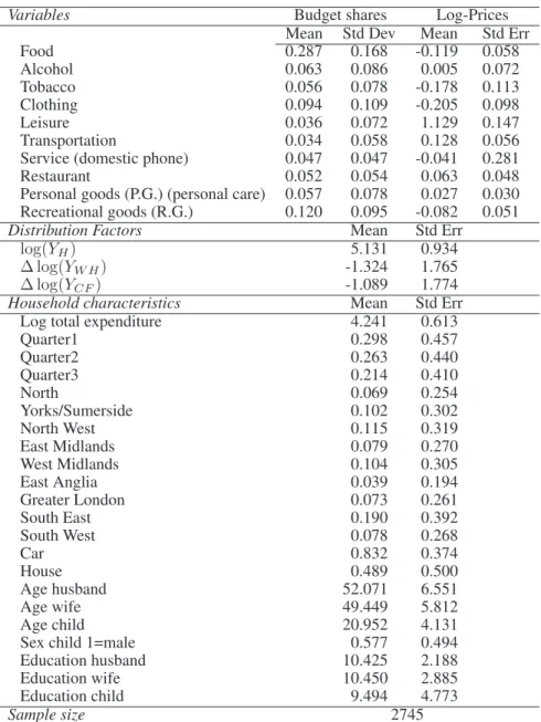
(13) separability, while restrictive, is common in the literature [see Banks et al. (1997)]. In addition, we condition the demand equations on home and car ownership to test a certain form of separability between durable and non-durable goods as shown below. The demand system we estimate comprises 11 categories of non-durable goods: food, restaurant meals, alcohol, tobacco, services, leisure, heating, transportation, clothing, recreational goods, and personal goods. With respect to the theoretical model, our demand system is thus characterised by 𝑆 = 2 and 𝑁 = 11. Prices are measured monthly at the country level, yielding 144 (12 years × 12 months) different prices for each good. Also we use 2-week expenditure data. Testing Proposition 3 in this context requires observing at least three distribution factors. Given the composition of households, and in light of the fact that the demand system is conditioned on total expenditure on non-durable goods, we can construct three distribution factors from individual incomes. Following BC1998, we use the log of the husband’s gross income, log(𝑌𝐻 ), the difference between the log of the wife and the husband’s income, Δ log(𝑌𝑊 𝐻 ), and the difference between the log of the child’s and the father’s income, Δ log(𝑌𝐶𝐻 ).12 Of course, these variables need to be used cautiously since their validity as distribution factors depends on the assumption of separability. Nonetheless, they may have a significant impact on the decision-making process at the household level for given total expenditures on non-durable goods. Other factors could eventually be included in the analysis (e.g. sex ratio, divorce laws, minimum wage, age at which a youngster can drive a car, youth unemployment rate, etc.). In this paper, the analysis is limited to the above distribution factors. Table 1 presents the descriptive statistics of our sample. These statistics are compiled for all the years from 1982 to 1993. Since we omit durable goods, it is not surprising that the largest shares relate to food, recreational goods, and clothing. Moreover, the distribution factors suggest a significant gap between the spouses’ income on one hand, and between the father’s and the child’s income, on the other. Other variables in the table reveal that the majority of households have a car (83.2%) and about half own a house (48.9%). Finally, the spouses’ education levels are similar, while the children are slightly less educated presumably because of their age. Price variability (as measured by standard errors) varies across goods. It is relatively large for leisure (= 43.1), tobacco (= 9.8), clothing (= 7.8) and alcohol (= 7.4). However, it is much smaller for service (= 2.7), personal goods (= 3.1) and recreational goods (= 4.6). While low price variability of certain goods is likely to make identification of price effects more difficult, our empirical results show that a large number of estimated price coefficients are statistically significant (see section 4).. 3.2 The Empirical Model To implement the empirical tests, we estimate a Quadratic Almost Ideal Demand System (QUAIDS) as proposed by Banks et al. (1997) and used by BC1998. The QUAIDS model has the advantage of being a flexible functional form that accommodates quadratic nonlinearities in the Engel curves. More specifically, it is a rank three demand system in the sense of Lewbel (1991). Also, it has been validated empirically on many occasions [e.g., Banks et al. (1997); Blundell and Robin (1999); Browning et al. (2007)]. 12 BC1998 do not include the third distribution factor because they assume that only the spouses are potential decision-makers in the household.. 9.

(14) Table 1: Descriptive Statistics Variables. Budget shares Log-Prices Mean Std Dev Mean Std Err Food 0.287 0.168 -0.119 0.058 Alcohol 0.063 0.086 0.005 0.072 Tobacco 0.056 0.078 -0.178 0.113 Clothing 0.094 0.109 -0.205 0.098 Leisure 0.036 0.072 1.129 0.147 Transportation 0.034 0.058 0.128 0.056 Service (domestic phone) 0.047 0.047 -0.041 0.281 Restaurant 0.052 0.054 0.063 0.048 Personal goods (P.G.) (personal care) 0.057 0.078 0.027 0.030 Recreational goods (R.G.) 0.120 0.095 -0.082 0.051 Distribution Factors Mean Std Err log(𝑌𝐻 ) 5.131 0.934 Δ log(𝑌𝑊 𝐻 ) -1.324 1.765 Δ log(𝑌𝐶𝐹 ) -1.089 1.774 Household characteristics Mean Std Err Log total expenditure 4.241 0.613 Quarter1 0.298 0.457 Quarter2 0.263 0.440 Quarter3 0.214 0.410 North 0.069 0.254 Yorks/Sumerside 0.102 0.302 North West 0.115 0.319 East Midlands 0.079 0.270 West Midlands 0.104 0.305 East Anglia 0.039 0.194 Greater London 0.073 0.261 South East 0.190 0.392 South West 0.078 0.268 Car 0.832 0.374 House 0.489 0.500 Age husband 52.071 6.551 Age wife 49.449 5.812 Age child 20.952 4.131 Sex child 1=male 0.577 0.494 Education husband 10.425 2.188 Education wife 10.450 2.885 Education child 9.494 4.773 Sample size 2745 Note : The amounts are expressed in sterling pounds.. 10.

(15) The budget shares are written as: 𝑤 = 𝜶 + Θy + Γ𝒑 + 𝜷 (ln(𝑚) − 𝑎(𝒑)) + 𝝀. (ln(𝑚) − 𝑎(𝒑))2 + 𝝊, 𝑏(𝒑). (3). where 𝜶, 𝜷 and 𝝀 are (𝑁 × 1) vectors of parameters, Θ and Γ are (𝑁 × 𝐾) and (𝑁 × 𝑁 ) matrices of parameters, respectively, 𝒚 is a (𝐾 × 1) vector of distribution factors, 𝒑 is an (𝑁 × 1) vector of log prices, ln(𝑚) is the log of the household’s total expenditure on non-durable goods, and 𝝊 is a vector of error terms. The price indexes 𝑎(𝒑) and 𝑏(𝒑) are defined as: 1 𝑎(𝒑) = 𝛼0 + 𝜶′ 𝒑 + 𝒑′ Γ𝒑 2 𝑏(𝒑) = exp(𝜷 ′ 𝒑).. (4) (5). Additivity implies that 𝜶′ 𝒆 = 1, Θ′ 𝒆 = 0 and 𝜷 ′ 𝒆 = 𝝀′ 𝒆 = Γ𝒆 = 0, where 𝒆 is an 𝑁 -dimensional unit vector. Homogeneity implies Γ′ 𝒆 = 0. In practise, additivity necessarily obtains owing to the construction of the data in terms of budget shares. Thus we estimate a system of 10 equations rather than 11 by arbitrarily eliminating one equation from the system (heating). The parameters of the omitted equation are obtained by substitution into the budget constraint. To simplify notation, we let 𝑁 = 10 in what follows. We impose homogeneity by substituting relative prices for absolute prices (we divide them all by the price of heating, the reference price). In equation (3), the distribution factors are introduced so as to only impact the constants in the share equations. The Pseudo-Slutsky matrix is given by: ( ) 𝑚 ˜ 𝑳=Γ − 𝜷 + 2𝝀 𝒑′ (Γ − Γ′ ) 𝑏(𝒑) } { ( ) 𝑚 ˜ 2 𝑚 ˜ ′ ′ ′ ′ (𝝀𝜷 + 𝜷𝝀 ) + 𝝀𝝀 , + 𝑚 ˜ 𝜷𝜷 + 𝑏(𝒑) 𝑏(𝒑) 1 2. (6). with 𝑚 ˜ = ln(𝑚)−𝑎(𝒑). So far we have omitted preference variables that take into account observable individual heterogeneity. In the empirical specification, we incorporate a vector 𝒛 of socio-demographic characteristics through the functions 𝑎(𝒑) and 𝑏(𝒑). More precisely, we write: 1 𝑎(𝒑, 𝒛) = 𝛼0 + 𝜶(𝒛)′ 𝒑 + 𝒑′ Γ𝒑, and ( ) 2 𝑏(𝒑, 𝒛) = exp 𝜷(𝒛)′ 𝒑 ,. (7) (8). where the functions 𝜶(𝒛) and 𝜷(𝒛) are linear in 𝒛, a vector of control variables. The vector 𝒛 includes a series of dummy variables (nine regional variables, three seasonal dummies, car and home ownership).13 The linearity of the QUAIDS model(3) is conditional on the terms 𝑎(𝒑) and 𝑏(𝒑). Consequently, it can be directly estimated using iterated ordinary least squares as proposed by Blundell and Robin (1999). The approach consists in estimating the demand system by OLS, conditional on a given set of initial parameter values Γ0 and 13. Preliminary estimations revealed that education and age were never jointly significant, possibly owing to the homogeneity of the sample. They are thus left out of 𝜶(𝒛) and 𝜷(𝒛) but are used as identifying instruments. See footnote 21.. 11.

(16) 𝜶0 that are substituted into in 𝑎(𝒑) and 𝑏(𝒑). The conditional OLS parameters Γ1 and 𝜶1 are next substituted in 𝑎(𝒑) and 𝑏(𝒑) and a new set of conditional OLS parameters Γ2 and 𝜶2 are estimated. The process is repeated until the conditional OLS parameters Γ𝑖+1 and 𝜶𝑖+1 are equal to those of the previous round, i.e. Γ𝑖 and 𝜶𝑖 . To account for the possibility that the log of total expenditure on non-durable goods is endogenous14 , we include the residuals of an auxiliary regression of the log of total expenditure on a set of instruments into the QUAIDS specification in (3).15 Conditional on this additional regressor, the so-called control function, the expenditure variable is exogenous. In this approach, the error term 𝝊 can be written as the orthogonal decomposition 𝝊 = 𝜌𝑢 + 𝜖.. (9). Testing 𝜌 = 0 is equivalent to a test for the exogeneity of the log of total expenditure on non-durables.16. 4. Estimation Results. The main purpose of the paper is to investigate the extent to which adolescent and older children exert some influence on household consumption choices. The empirical strategy must necessarily rest on a sample of households in which children interact with their parents. It could be argued that the household composition is precisely determined by the relative bargaining power of its members. In other words, children who live with their parents may do so precisely because their bargaining power is strong. Those who did not enjoy such an enviable situation may have left the family nest. In statistical terminology, our sample may suffer from self-selection problems.17 In our particular framework the direction of the bias is ambiguous however. Some children may have left the family nest because they enjoyed a good outside option. Others may have left because their parents had a very good threat point. Excluding children from the former group will underestimate the decision-making power of children. Excluding children from the latter group will overestimate the bargaining position of children. We investigate this issue by stratifying our sample into two groups.18 The first includes households in which the child is aged between 16 and 21 years. The second includes children that are at least 22 years of age. Since the probability of leaving the family nest is lower for the younger group, this sample is less likely to suffer from selectivity bias. The parameter estimates of the demand system for the complete sample are presented in Table 2. The first 14. It is sometimes argued that prices could also be considered as endogenous. This is likely to arise when the analysis focuses on firms since prices for individual goods can be thought to be set while targeting (partially unobserved) characteristics of individual consumers. In our application, however, we consider broad aggregates of goods and we expect such effects to wash out. Moreover, following the recent microeconometric demand literature we consider atomic individuals that act as price takers, and we control for time effects. This is why we concentrate on the endogeneity of total expenditure. Hoderlein (2009) and Haag et al. (2009) similarly treat total expenditure as endogenous and prices as exogenous. 15 After some experimentation, and following Banks et al. (1997), we chose not to include a residual generated by a regression of the square of expenditure on the instruments as an additional variable. 16 We also tested the exogeneity of the distribution factors using the same approach. The exogeneity of each distribution factor could not be rejected in every demand equation (except transportation). These results are not reported for the sake of brevity but are available upon request. 17 Note that this problem applies equally well to unitary and non-unitary models because the analysis is always carried out conditionally on household composition. The same problem arises when studying couples because the decision to marry or to divorce is also endogenous in most models. The same criticism may be addressed at all the tests of the collective model that have been conducted so far in the literature. 18 We can not correct for this potential selection bias since we have no information on children who left the household.. 12.

(17) panel of the table reports the parameter estimates of the distribution factors (Θ). The second panel focuses on the price variables (Γ). The regression also includes a series of control variables, 𝒛, which includes dummy variables for home and car ownership, 9 regional dummy variables, and 3 seasonal dummy variables, and that are not reported for the sake of brevity. Each distribution factor has a significant impact on at least two demand equations. For instance, an increase in the husband’s income (log 𝑌𝐻 ) translates into more being spent on food and less on recreational goods. Likewise, as the wife’s income increases relative to that of her husband (Δ log(𝑌𝑊 𝐻 )) more is spent on food and less on leisure goods. Finally, as the children’s income increase relative to their father’s (Δ log(𝑌𝐶𝐻 )), more is spent on tobacco and less is spent on recreational goods. The second panel of the table shows that a large number (42/100) of the prices variables parameters are statistically significant.19 Except for the Transportation equation, all the own-price parameter estimates that are significant are negative as expected.20 The last panel of the table reports two specification tests. The first line concerns the exogeneity of total expenditure. As mentioned before the residuals from an auxiliary regression of total expenditure on a series of instrumental variables are included as an explanatory variable.21 The parameter estimates are statistically different from zero in all but one equation (Transportation), thus rejecting the exogeneity assumption. The second line of the panel reports the 𝜒2 statistics of the joint test of the validity of instruments and of the over-identifying restrictions. According to the table neither hypotheses can be rejected. Tables 4–7 in appendix report the parameter estimates for the samples of households whose child is female, male, aged between 16–21, and aged 22 and over, respectively. The estimates of the price variables are relatively similar across the tables. The main differences relate to the parameter estimates of the distribution factors. The relative income of daughters (Table 4) increases the consumption of tobacco products but no such effect are found in the sample of sons (Table 5). Interestingly we find that an increase in the wife’s relative income increases the consumption of alcohol when the child is female. Conversely, when the child is male the father’s relative income decreases the consumption of alcohol. Perhaps surprisingly, the relative income of the sons has a negative and significant impact on the consumption of recreational goods. A similar result holds for the samples of daughters and both age groups, although the parameter estimate is only statistically significant at 15% for daughters and the children aged 22 and over. The parameter estimates of the price effects are simply too numerous to make any worthwhile inference. Systematic differences can only be ascertained through formal statistical tests.. 4.1 Testing the collective model and determining the number of decision-makers Propositions 2 and 3 provide two independent tests of the collective model. The former is based upon the price effects, Γ, while the latter is based upon distribution factor effects, Θ. In testing the rank of these matrices, we follow a sequential approach. In the context of Proposition 2, we first start by testing 𝐻0 : rank(𝑴 ) = 0, that is, the unitary model.22 If the null hypothesis is rejected, we then test 𝐻0 : rank(𝑴 ) = 2, the collective model 19. Preliminary estimates revealed that the assumption of homogeneity cannot be rejected. Note that the matrix Γ is not required to be negative semi-definite in eq. (3) even in the unitary model (see Banks et al. (1997)). 21 In addition to the explanatory variables and the distribution factors, the instrumental variables are: age, age2 , age3 , education, education2 , education3 of both spouses, a yearly trend, and the log of the price index. 22 Note that the unitary model is also a collective model with at least one decision maker. However, following the standard literature in household economics, we refer to this model as the unitary model. 20. 13.

(18) 14 -0,131 (25,924) 10,963. 0,009 (2,964) 8,736. -0,079 (1,276) -0,030 (1,270) 0,089 (4,048) 0,052 (1,460) 0,009 (0,639) -0,294 (3,941) 0,087 (0,402) -0,516 (3,869) 0,556 (2,795) -0,146 (0,987). -0,002 (1,131) 0,000 (0,408) 0,000 (0,088). Alc.. -0,009 (3,622) 7,547. -0,072 (1,396) -0,059 (3,031) 0,027 (1,438) 0,026 (0,852) -0,019 (1,610) 0,027 (0,437) -0,288 (1,578) -0,076 (0,674) 0,269 (1,607) 0,114 (0,915). 0,002 (1,173) 0,000 (0,303) 0,002 (2,109). Tobac.. Leisure Trans. Serv. D ISTRIBUTION FACTORS -0,002 -0,002 -0,002 0,000 (0,919) (1,236) (1,201) (0,285) 0,000 -0,002 -0,001 0,000 (0,356) (2,057) (0,890) (0,298) 0,001 0,000 0,000 0,000 (0,568) (0,212) (0,433) (0,120) P RICE VARIABLES -0,018 0,139 0,102 -0,113 (0,249) (2,644) (2,293) (3,079) 0,001 0,010 0,032 -0,005 (0,031) (0,484) (1,876) (0,364) 0,032 -0,013 -0,003 -0,141 (1,263) (0,721) (0,196) (10,849) 0,006 -0,055 -0,027 0,024 (0,152) (1,824) (1,048) (1,139) 0,034 -0,024 0,020 -0,025 (2,143) (2,088) (1,968) (3,006) 0,387 0,195 0,123 -0,093 (4,522) (3,070) (2,277) (2,095) 0,578 0,555 0,138 0,090 (2,323) (3,006) (0,882) (0,698) -0,615 -0,460 -0,162 0,262 (4,012) (4,042) (1,673) (3,305) -0,053 -0,085 -0,144 -0,186 (0,231) (0,504) (0,996) (1,578) -0,098 -0,157 -0,095 0,219 (0,579) (1,247) (0,884) (2,495) S PECIFICATION T ESTS‡ 0,021 0,038 -0,004 -0,012 (6,016) (14,367) (1,692) (6,670) 1,830 3,792 1,113 12,668. Cloth.. -0,005 (2,277) 0,762. 0,004 (0,093) 0,003 (0,163) 0,002 (0,111) 0,025 (1,014) 0,010 (1,123) 0,101 (2,001) -0,048 (0,325) -0,005 (0,051) -0,063 (0,467) 0,015 (0,151). 0,002 (1,179) 0,001 (1,092) 0,000 (0,090). Rest.. -0,021 (6,677) 8,019. 0,062 (0,996) 0,016 (0,675) 0,060 (2,723) 0,018 (0,492) 0,013 (0,947) -0,174 (2,322) 0,282 (1,295) 0,114 (0,847) -0,068 (0,341) -0,364 (2,444). 0,001 (0,668) 0,000 (0,065) 0,001 (0,959). P.G.. 0,015 (4,527) 16,279. 0,199 (3,085) -0,044 (1,812) 0,003 (0,148) -0,044 (1,183) -0,020 (1,372) 0,167 (2,134) 0,186 (0,818) 0,026 (0,189) -0,003 (0,014) -0,352 (2,265). -0,005 (2,483) 0,001 (1,497) -0,003 (3,629). R.G.. ‡. Asymptotic t statistics in parentheses. The first line reports the parameter estimates of the residuals from an auxiliary regression of total expenditures on a series of instrumental variables. The second line reports the 𝜒2 statistics of the over-identification test of the instrumental variables.. †. Total Expend (Residual) T-Stat. Over-Ident. 𝜒2(8). Γ-Recreational. Γ-Personal. Γ-Restaurant. Γ-Services. Γ-Transportation. Γ-Leisure. Γ-Clothing. Γ-Tobacco. Γ-Alcohol. Γ-Food. Δ log(𝑌𝐶𝐻 ) -0,527 (5,190) -0,069 (1,808) 0,000 (0,006) 0,101 (1,723) 0,069 (3,052) -1,120 (9,103) -2,645 (7,403) 1,390 (6,311) 1,230 (3,745) 0,893 (3,656). 0,011 (3,614) 0,003 (1,842) 0,001 (0,382). log(𝑌𝐻 ). Δ log(𝑌𝑊 𝐻 ). Food. Variable. Table 2: Parameter Estimates of the Demand System – Full Sample†.

(19) with at least two decision- makers.23 If this null hypothesis is again rejected we next test 𝐻0 : rank(𝑴 ) = 4, the collective model with three decision-makers. If all three ranks are rejected, we must reject collective rationality since rank(𝑴 ) must be at most 2𝑆, and we know that 𝑆 = 2. Otherwise, we do not reject collective rationality. We proceed in a similar fashion with Proposition 3. In the event that the collective model is not rejected by either sets of tests, Proposition 4 can be verified when rank(𝑴 ) = 2𝑆, that is, equal to 4. If Proposition 4 is rejected, the collective model is rejected. 4.1.1. Tests based on price variations. Testing the rank of 𝑴 ≡ 𝐿 − 𝐿′ is a relatively demanding task. Fortunately, in the context of the QUAIDS ′ specification, it can be shown that 𝐿 − 𝐿′ reduces to Γ − Γ under collective rationality [BC1998]. Therefore our strategy consists in testing sequentially the following null assumption for 𝐻 = 0, 1, 2: 𝐻0 : rank(𝑴 ) = 2𝐻, 𝐻𝐴 : rank(𝑴 ) > 2𝐻, ′. where 𝑴 = Γ − Γ . Let us study each step in turn. ∙ rank(𝑴 ) = 0 (Unitary model) Testing that the antisymmetric matrix 𝑴 has rank 0 is equivalent to testing the symmetry of the matrix Γ. Recall that the matrix Γ is (10×10). There are thus 10×(10−1)/2 = 45 linear constraints that must be satisfied. ∙ rank(𝑴 ) = 2 (Collective model with at least two decision-makers). Because the matrix 𝑴 is antisymmetric, all the elements on its main diagonal are zero. BC1998 exploit this property and have shown (their Lemma 3) that this is equivalent to testing that for all (𝑖, 𝑘) such that 𝑘 > 𝑖 > 2 the following equalities hold (assuming without loss of generality that 𝑚12 ∕= 0):. 𝑚𝑖𝑘 =. 𝑚1𝑖 𝑚2𝑘 − 𝑚1𝑘 𝑚2𝑖 , 𝑚12. where 𝑚𝑖𝑘 is the 𝑖𝑘 𝑡ℎ element of 𝑴 . Under rank(𝑴 ) = 2, as many as 28 constraints must be satisfied. ∙ rank(𝑴 ) = 4 (Collective model with three decision-makers). 23. Recall that the rank of the matrix 𝑴 is even since it is antisymmetric.. 15.

(20) As above, let 𝑴 = {𝑚𝑖𝑘 }, 𝑖, 𝑘 = 1, . . . , 10. Without loss of generality, assume further that: ¯ ¯ 0 𝑚12 𝑚13 𝑚14 ¯ ¯ ¯ −𝑚12 0 𝑚23 𝑚24 ∣𝑴4×4 ∣ = Det ¯¯ 0 𝑚34 ¯ −𝑚13 −𝑚23 ¯ ¯ −𝑚14 −𝑚24 −𝑚34 0. ¯ ¯ ¯ ¯ ¯ ¯ ∕= 0. ¯ ¯ ¯ ¯. It can be shown that 𝑴 has rank 4 if and only if ∀ 𝑘 > 𝑖 > 4 the following holds:. 𝑚𝑖𝑘 = {𝑚12 (𝑚3𝑖 𝑚4𝑘 − 𝑚3𝑘 𝑚4𝑖 ) + 𝑚13 (𝑚2𝑘 𝑚4𝑖 − 𝑚2𝑖 𝑚4𝑘 ) 𝑚14 (𝑚2𝑖 𝑚3𝑘 − 𝑚2𝑘 𝑚3𝑖 ) + 𝑚1𝑖 (𝑚23 𝑚4𝑘 − 𝑚24 𝑚3𝑘 + 𝑚2𝑘 𝑚34 ) + 𝑚1𝑘 (−𝑚23 𝑚4𝑖 − 𝑚24 𝑚3𝑖 − 𝑚2𝑖 𝑚34 )} /(𝑚12 𝑚34 − 𝑚13 𝑚24 + 𝑚14 𝑚33 ).. The denominator of the last expression corresponds to the square root of ∣𝑴4×4 ∣. Under rank(𝑴 ) = 4, 15 𝑚𝑖𝑘 constraints must be satisfied. Simple Wald tests can be computed to determine whether the above constraints are satisfied or not. The main advantage of this statistic is that it does not require the model to be estimated under the null hypothesis as opposed to the LR test or the Lagrange multiplier test. This is definitely important because the restrictions under rank(𝑴 ) = 2, and especially under rank(𝑴 ) = 4, are highly nonlinear and too complex to implement. Evidently the main weakness of the Wald test is that, in finite samples, it is not invariant to an algebraically equivalent parameterization of the null hypothesis.24 4.1.2. Tests based on distribution factors. The literature contains several statistical tests to determine the rank of a matrix [e.g., Gill and Lewbel (1992), Cragg and Donald (1997) and Robin and Smith (2000)].25 We follow a procedure that was recently proposed by Kleibergen and Paap (2006) and that is based on the singular value decomposition. The basic idea of their approach is to test how many singular values are significantly different from 0. Recall that the rank of a matrix is given by the number of its non-zero singular values. Let Θ′ be the 𝐾 × 𝑁 transposed matrix of distribution factor effects (with 𝑁 > 𝐾). It admits a singular values decomposition: Θ′ = 𝑈 Σ𝑉 , where 𝑈 is a 𝐾 × 𝐾 orthonormal matrix, 𝑉 is a 𝑁 × 𝑁 orthonormal matrix, and Σ is a 𝐾 × 𝑁 matrix whose main diagonal contains the singular values of Θ′ . Under the null hypothesis that rank(Θ) = 𝐻, (𝐻 = 0, ..., 𝐾 − 1), they construct a statistic based on an orthogonal transformation of the smallest (𝐾 −𝐻) singular values and on the inverse of the corresponding covariance matrix. The limiting distribution of the test statistic is 𝜒2(𝐾−𝐻)(𝐾−𝐻) . 24. There exists an extensive literature on this issue, e.g., Gregory and Veall (1985), Phillips and Park (1988), and Agüero (2008). This problem does not seem to be serious in our setup, given the large size of our samples. We performed a number of experiments with various algebraic transformations of our constraints. Our tests proved qualitatively robust to these transformations. 25 The test proposed by Gill and Lewbel (1992) is sensitive to the ordering of the variables in the matrix to be tested. In Cragg and Donald (1997), the test statistic is obtained using a numerical optimisation procedure which is not necessarily precise with relatively large matrices. Finally, the test statistic proposed by Robin and Smith (2000) does not follow a standard distribution, making the test procedure difficult to implement.. 16.

(21) This allows to test the null against the alternative rank(Θ) > 𝐻. To perform the test sequentially, the most constraining null hypothesis is first tested (i.e.,rank(Θ) = 0), which corresponds to the unitary model. If rejected, the next most restrictive null hypothesis is tested and so on. As predicted by Proposition 3, the collective model is rejected if one rejects that rank(Θ) = 𝑆, which is equal to 2 in our case. One advantage of this test is that, contrary to the Wald test, it is invariant to an arbitrary reparameterization of the null hypothesis. Its main disadvantage is that it can not be used to test the rank of antisymmetric matrices such as 𝑴 in Proposition 2.26 4.1.3. Tests Based on Price Variations and Distribution Factors. Proposition 4 implies that Θ and the columns of 𝑴 are collinear when rank(𝑴 ) = 2𝑆. The collinearity can be easily ascertained using the test procedure proposed by Kleibergen and Paap (2006). Let Ξ stand for the horizontal concatenation of 𝑴 and Θ, i.e., Ξ = 𝑴 ∣Θ. Their test procedure can be applied to investigate the rank of Ξ since the matrix is not antisymmetric. Under the null assumption of collective rationality with rank(𝑴 ) = 2𝑆 (𝑆 + 1 decision-makers), it should be equal to 2𝑆.. 4.2 Tests Results Table 3 reports the test results. The table is divided into three sections, each corresponding to Propositions 2, 3 and 4, respectively. Column (1) reports the test result for rank(𝑴 ) = 0, i.e. that the household behaves according to the unitary model. The column indicates that the assumption is strongly rejected for all five samples we have considered. Columns (2) and (3) report the 𝜒2 statistics for rank(𝑴 ) = 2 and rank(𝑴 ) = 4, that is, collective rationality with at least two decision-makers and three decision-makers, respectively. Column (2) shows very interesting results. First, it appears that the collective model with at least two decision-makers must be rejected when using the whole sample. The 𝜒2 statistic is equal to 62.6 and the associated p-value is approximately equal to .0002. The same conclusion prevails with the sample of children aged between 16 and 22. When the model is estimated with the sample of daughters, the test statistic has a p-value equal to 0.049. The model is thus marginally rejected at the 5% level and relatively easily rejected at the 10% level. Interestingly, the collective model with at least two decision-makers cannot be rejected with either the sample of sons and the sample of children aged 22 and older. This does not imply that these children are not decision-makers within their household. Rather, the results imply that we can not reject that they do not take part in the family decision-making process. The possibility that children aged 22 and over may not be decision-makers could be explained by the unwillingness of parents to negotiate with them once they reach a certain age and would prefer that they leave the family nest. As was stressed earlier, this sample is the most likely to suffer from selection bias. 26. The eigenvalues of antisymmetric (or skew symmetric) matrices such as 𝑴 are either 0 or pure imaginary so the limiting distributions of the test will not be 𝜒2 in general. The test proposed by (Kleibergen and Paap, 2006) can not be used to determine the rank of 𝑴 .. 17.

(22) Table 3: 𝜒2 Test Statistics. (Rank) (DF) S AMPLE : Complete Daughters Sons Children 16–21 Children 22+ †. Rank of 𝑴. Rank of Θ. Rank of (𝑴 ∣Θ). (Proposition 2). (Proposition 3). (Proposition 4). 0 45 (1). 2 28 (2). 4 15 (3). 0 30 (4). 1 18 (5). 2 8 (6). 4 54 (7). 445.549 (0.000) 277.261 (0.000) 221.508 (0.000) 298.235 (0.000) 186.407 (0.000). 62.599 (0.000) 41.350 (0.049) 27.261 (0.504) 49.132 (0.008) 23.254 (0.720). 3.981 (0.998) 1.923 (0.999). 111.397 (0.000) 116.751 (0.000) 54.735 (0.004) 107.351 (0.000) 143.201 (0.000). 48.837 (0.000) 31.367 (0.026) 20.508 0.305 31.958 (0.022) 21.195 (0.270). 1.445 (0.994) 3.943 (0.862). 54.622 0.451 53.178 (0.506). 1.355 (0.995). 45.227 (0.797). 2.135 (0.999). Probability under the null between parentheses.. Column (3) reports the test statistics based on the null hypothesis of collective rationality with three decisionmakers. Following our sequential approach, the test statistics are only reported for those household configurations for which the null hypothesis that there are at least two decision-makers is rejected. Interestingly, in the three cases where this occurs, the null hypothesis cannot be rejected. We must thus conclude on the basis of the rank of 𝑴 that the collective model with three decision-makers is supported for the complete sample, and in particular for the sub-samples of daughters and children aged between 16 and 21. It is rather puzzling that daughters appear to exert a clear influence on the decision-making process while the evidence is much weaker for sons. From a bargaining point of view it could be argued that the daughters’ threat point is likely higher because they tend to marry at a younger age with a potentially older spouse with greater earnings. The second section of the table focuses on Proposition 3, i.e. the impact of the distribution factors. The 𝜒2 test statistics reported in columns (4)–(6) are all based upon the test proposed by Kleibergen and Paap (2006). According to the table, the null hypothesis that the rank of Θ is equal to zero is rejected in all cases at the 5% level of significance. As with Proposition 2, the unitary model is thus strongly rejected. According to Column (5), Proposition 3 yields identical results to those of Proposition 2. Indeed, the data reject the null hypothesis that there are at least two decision-makers when the model is estimated with the complete sample, the sample of daughters and the sample of children aged between 16 and 21. Likewise, they do not reject the null hypothesis that there are at least two decision-makers when considering the sample of sons or the sample of children aged 22 and above. Column (6) further indicates that when the model is estimated with either the complete sample, the sample of daughters, or the sample of children aged 16–21, the null hypothesis that the rank of Θ is equal to two can not rejected. Therefore, the specifications based on these samples are also consistent collective rationality and with there being three decision-makers in the households. The last column of the table reports the test statistics based on the null hypothesis that there are three decision-. 18.

(23) makers in the household and that the distribution factors effects are collinear with the price effects.27 The test statistics are reported only for the samples that satisfy collective rationality with three decision-makers, i.e. complete, daughters and children 16–21. According to the test result, it must be concluded that the consumption behaviour of these households can be rationalised by a collective model with three decision-makers.28. 5. Conclusion. To the best of our knowledge, this paper is the first to test the hypothesis of Pareto efficiency in households comprising potentially more than two decision-makers and using data from a developed country. It is also the first to treat children aged 16 and over and living with their parents as regular decision-makers. We first present an overview of the tests that have recently been developed in the literature to test the collective rationality within multi-person households. These are based on the impact of prices and distribution factors on household demands. Intuitively, prices and distribution factors affect the demands indirectly through the so-called individual Pareto weights. The fact that there are only as many Pareto weights as there are potential decisionmakers imposes specific constraints on the rank of the compensated price and factor distributions effects. The framework we use is general enough to analyse the consumption choices of a variety of household types including, but not limited to, couples living with grown-ups, adult children, elderly parents, etc. In the paper we focus on the non–durable consumption expenditures of households composed of two parents and a single child of at least 16 years of age living with his parents. The sample is drawn from a series of U.K. Family Expenditure Surveys covering the period 1982–1993. We acknowledge that household composition may be partly determined by the relative bargaining power of its members. In particular, adult children may choose to live with their parents because they enjoy an enviable position. Plainly stated, our sample may be plagued by self-selection problems. We investigate this issue by stratifying our sample into two groups: (1) households in which the child is aged between 16 and 21; (2) households whose child is at least 22 years of age. We also stratify the sample by gender to investigate whether sons and daughters have similar bargaining power within the household. The empirical analysis yields a number of interesting results. First, the collective model is not rejected for any of the samples we have considered. This result is consistent with recent non-parametric tests of the model (e.g., Cherchye et al. (2009)). Second, our estimates provide strong evidence that households with a child aged 16 and over behave as tough there are three decision-makers. Third, when the analysis is stratified by age and by gender, this result also holds in households whose child is aged between 16 and 21. This result underlines the importance of recognising the input of adolescent children into the family decision-making process. Daughters are similarly found to affect the consumption decisions, irrespective of their age. The consumption pattern of households whose child is at least 22 years of age, and those whose child is male, while compatible with collective rationality, is only consistent with there being at least two decision-makers. 27. The 𝜒2 statistics are based upon the Kleibergen and Paap (2006) test. The p-values reported in column (3) (𝐻0 : rank(𝑴 ) = 4) are very close to 1. This may suggest that the power of the Wald test is low despite the samples being relatively large. While this possibility may not be ruled out, the test nevertheless rejects the null hypothesis in three out of five case when testing 𝐻0 : rank(𝑴 ) = 2 and in all cases when testing 𝐻0 : rank(𝑴 ) = 0. Similarly, the p-values of the 𝜒2 statistics that test rank(Θ) = 2 are very close to one except for the sample of daughters. Just as with the Wald test, the test statistics based upon the work of Kleibergen and Paap (2006) are capable of strongly rejecting the null assumptions in some cases (complete sample, daughters, children 16–21) while failing to reject in other cases (sons and children 22 and over). The consistency of the test results across different household configurations lends them a certain credibility. 28. 19.

(24) All in all, our analysis underlines the fact that it may be incorrect to assume that there are no more than two decision-makers when a household comprises children aged 16 and over. This hypothesis has never been tested rigorously before and is routinely made in virtually every empirical analysis of household consumption. Clearly, the assumed number of decision-makers is very important for intra-household welfare analysis and policy targeting. Acknowledging that children may influence the household decision-making process could prove important to the way we approach these issues.. 20.