Centre de Recherche en économie de l’Environnement, de l’Agroalimentaire, des Transports et de l’Énergie
Center for Research on the economics of the Environment, Agri-food, Transports and Energy
_______________________
Gaigné: Corresponding author. INRA, UMR1302 SMART, 35000 Rennes (France) and CREATE, Université Laval, Québec, Canada [email protected]
Riou: GATE Lyon-Saint-Etienne; Université de Lyon (France); Université Jean Monnet, Saint-Etienne [email protected]
Thisse: CORE, Université Catholique de Louvain (Belgium), CREA, Université du Luxembourg, and CEPR [email protected]
The authors thank William Strange and two referees for their suggestions that have allowed for major improvements in the presentation of this paper. We are also grateful to S. de Clara, K. Chen, H. Overman, S. Proost, P. Rietveld, K. Vandender, H. Wenban-Smith, and seminar audience at the London School of Economics and National University of Singapore for stimulating comments and discussions.
Professor Gaigné is visiting us a CREATE from August 2011 to July 2012.
Les cahiers de recherche du CREATE ne font pas l’objet d’un processus d’évaluation par les pairs/CREATE working papers do not undergo a peer review process.
ISSN 1927-5544
Are Compact Cities Environmentally (and Socially)
Desirable ?
Carl Gaigné
Stéphane Riou
Jacques-François Thisse
Cahier de recherche/Working Paper 2012-4
Abstract:
There is a wide consensus among international institutions and national governments in favor of compact (i.e. densely populated) cities as a way to improve the ecological performance of the transport system. Indeed, when both the intercity and intra-urban distributions of activities are given, a higher population density makes cities more environmentally friendly as the average commuting length is reduced. However, when we account for the possible relocation of activities within and between cities in response to a higher population density, the latter may cease to hold. Because changes in population density affect land rents and wages, firms and workers re-optimize and choose new locations. We show that this may reshape the urban system in a way that generates both a higher level of pollution and welfare losses. As cities become more compact, agglomeration occurs and, eventually, the secondary business centers vanish. By increasing the average commuting length, these changes in the size and structure of cities may be detrimental to both the ecological and welfare objectives even if intercity trade flows decrease. This means that compact is not always desirable, and thus an increasing-density policy should be supplemented with instruments that impact the intra- and inter-urban distributions of activities. We argue that a policy promoting the creation of secondary business centers can raise welfare and decrease emissions.
Keywords: Greenhouse gas, commuting costs, transport costs, cities Résumé:
Il existe un large consensus parmi les institutions internationales et les gouvernements nationaux en faveur des villes compactes (c’est-à-dire densément peuplées) comme un moyen d’améliorer la performance écologique de nos systèmes de transport. En effet, lorsque la localisation des activités demeure inchangée, une forte densité de population rend les villes plus respectueuses de l’environnement car la longueur du trajet moyen est réduite. Cependant, les effets à long terme sont incertains dans la mesure où la localisation des activités au sein et entre les villes s’ajuste en réponse à une forte densité de population. En effet, le changement de densité de population, en affectant les rentes foncières et les salaires, modifie la localisation des entreprises et des travailleurs, et donc la demande de transport. Nous montrons que la densification des villes peut remodeler le système urbain d’une manière qui détériore la situation environnementale et le bien-être. Des villes plus compacts accroissent la concentration spatiale et, éventuellement, réduisent la taille des pôles d’emploi secondaires. En augmentant la longueur de trajet en moyenne, ces changements dans la taille et la structure des villes peuvent être préjudiciables pour l’environnement et le bien-être, même si le commerce interurbain de marchandises diminue. Nous soutenons qu’une politique de promotion de la création de pôles d’emploi secondaires peut augmenter le bien-être et diminuer la pollution liée au transport.
Mots clés: Gaz à effet de serre, transport de marchandises, déplacement domicile/travail, villes compactes
1
Introduction
According to Yvo de Boer, former Executive Secretary of the United Nations, “Given the role that transport plays in causing greenhouse gas emissions, any serious action on climate change will zoom in on the transport sector” (speech to the Ministerial Conference on Global Environment and Energy in Transport, January 15, 2009). The transport sector is indeed a large and growing emitter of greenhouse gases (GHG). It accounts for 30% of total GHG emissions in the US and approximately 20% of GHG emissions in the EU-15 (OECD, 2008). Within the EU-27, GHG emissions in the transport sector have increased by 28% over the period 1990-2006, whereas the average reduction of emissions across all sectors is 3%. Moreover, road-based transport accounts for a very large share of GHG emissions generated by the transport sector. For example, in the US, nearly 60% of GHG emissions stem from gasoline consumption for private vehicle use, while a share of 20% is attributed to freight trucks, with an increase of 75% from 1990 to 2006 (Environmental Protection Agency, 2011).1
Although new technological solutions for some transport modes might allow for substantial reductions in GHG emissions (Kahn and Schwartz, 2008), improvements in energy e¢ ciency are likely to be insu¢ cient to stabilize the pollution level in the transport sector (European Environment Agency, 2007). Thus, other initiatives are needed, such as mitigation policies based on the reduction of average distances travelled by people and commodities. To a large extent, this explains the remarkable consensus among international institutions as well as local and national governments to foster the development of compact (or densely populated) cities as a way of reducing the ecological impact of cities and contributing to sustainable urban development. Nevertheless, the analysis of global warming and climate change neglects the spatial organization of the economy as a whole and, therefore, its impact on transport demand and the resulting GHG emissions. It is our contention that such neglect is unwarranted.
A large body of empirical literature highlights the e¤ect of city size and structure on GHG emissions through the level of commuting (Bento et al., 2006; Kahn, 2006; Brownstone and Golob, 2009; Glaeser and Kahn, 2010). The current trend toward increased vehicle use has been reinforced by urban sprawl, as suburbanites’ trips between residences and workplaces have increased (Brueckner, 2000; Glaeser and Kahn, 2004). Kahn (2006) reports that the predicted gasoline consumption for a representative household is lowest in relatively compact cities such as New York and San Francisco and is highest in sprawling cities such as Atlanta and Houston. While the environmental costs of urban sprawl are increasingly investigated in North America, the issue is becoming important in Europe as well. For example, between 1986
1This increase is associated with an increase in the average distance per shipment. In France, from 1975 à
1995, the average kilometers per shipment has increased by 38% for all transportation modes, and by 71% for road transport only (Savin, 2000). Similar evolutions have been observed in the richer EU countries and in the USA.
and 1996 in the metropolitan area of Barcelona, the level of per capita emissions doubled, the average trip distance increased by 45%, and the proportion of trips made by car increased by 62% (Muniz and Galindo, 2005). Recognizing the environmental cost of urban sprawl, scholars and city planners alike advocate city compactness as an ideal.2
Starting from the prevailing view that more compact cities is the proper way to contain GHG emissions, our paper addresses the following two issues. Firstly, when assessing the merits of increasing-density policies, the existing literature disregards one major problem: a higher population density may spark the relocation of …rms and households. Instead, a full-‡edged analysis of such a policy should be conducted within a framework in which …rms and households’locations are endogenously chosen in response to a higher population density. When its e¤ects on the spatial distribution of …rms and households are ignored, the environmental impact of an increasing-density policy is always positive because people commute over shorter distance. However, such a policy a¤ects prices, wages and land rents, which lead …rms and households to change places in order to re-optimize pro…ts and utility. Accounting for these spatial e¤ects makes the impact of higher urban density more ambiguous because their net e¤ects depend on whether the new spatial pattern is better or worse from the environmental viewpoint.
Secondly, once it is recognized that the desirability of increasing-density policies depends on the resulting spatial pattern, another question comes to mind: which spatial distribution of …rms/households minimizes transport-related GHG emissions in the space-economy as a whole? Transporting people and commodities involves environmental costs which are associated with the following fundamental trade-o¤: concentrating people and …rms in a reduced number of large cities minimizes pollution generates by commodity shipping among urban areas but increases pollution stemming from a longer average commuting; dispersing people and …rms across numerous small cities has the opposite e¤ects. Therefore a sound environmental policy should be based upon the ecological assessment of the entire urban system. Although seemingly intuitive, this global approach has not been part of the debate on the desirability of compact cities.
That said, the above trade-o¤ also has a monetary side, and thus an increasing-density policy has welfare implications that are often overlooked by compact cities’proponents. This should not come as a surprise because transporting people and commodities involves both economic and ecological costs. In other words, there is a tight connection between the ecological and welfare objectives. According to Stern (2008), the emissions of GHG are the biggest market failure that the public authorities have to manage. It is, therefore, tempting to argue that deadweight losses associated with market imperfections are of second order. This view is too extreme because a higher population density impacts the consumption of all goods, and thus
2See Dantzig and Saaty (1973) for an old but sound discussion of the advantages of compact cities. Gordon
changes individual welfare. Having this in mind, we show that increasing density may generate welfare losses when the urban system shifts from dispersion to agglomeration. For this reason, our paper focuses on both the ecological and welfare e¤ects of a higher population density when …rms and households are free to relocate between and within cities.
In doing so, we consider the following two urban scenarios. In the …rst one, cities are monocentric while consumers and …rms are free to relocate between cities in response to a higher population density. We show that an increasing-density policy may generate a hike in global pollution when this policy leads the urban economy to shift from dispersion to agglomeration, or vice versa. For example, when both the initial population density and the unit commuting cost are low enough, an increasing-density policy incentivizes consumers and …rms to concentrate within a single city. However, at this new spatial pattern, the density may remain su¢ ciently low for a single large city to be associated with a longer average commuting, which generates more pollutants than two small cities. Conversely, when the unit commuting cost is high, the market leads to the dispersion of activities because consumers aim to bear lower land rent and commuting costs. Yet, when the density gets su¢ ciently high, the average commuting is short enough for the agglomeration to be ecologically desirable because intercity transport ‡ows vanish. Consequently, agglomeration or dispersion is not by itself the most preferable pattern from the ecological point of view. In other words, our results question the commonly held belief of many urban planners and policy-makers that more compact cities are always desirable. They also show that one should pay more attention to the e¤ect of increasing-density policies on city size.
In the second scenario, we study the ecological and welfare impact of an increasing-density policy when both the city size and morphology are endogenously determined. By inducing high urban costs, a low population density leads to both the dispersion and decentralization of jobs, that is, the emergence of polycentric cities. If urban planners make the urban system more compact (i.e. raise population density), then, the secondary business centers shrink smoothly and, eventually, …rms and households produce and reside in a single monocentric city. We show that these changes in the size and structure of cities may generate higher emissions from commuting. Thus, an increasing-density policy should be supplemented with instruments that in‡uence the intra- and inter-urban distributions of households and …rms. In particular, we argue that a decentralization of jobs within cities, that is, a policy promoting the creation of secondary business centers, both raises welfare and decreases GHG emissions.
In what follows, we assume that the planner chooses the same population density in all cities. Alternately, we could assume that city governments noncooperatively choose their own population density. Both approaches have merits that are likely to suit countries with di¤erent attitudes regarding major issues such as the development of more densely populated cities. Our main argument is that the planning outcome is typically used by economists when assessing the costs and bene…ts of a particular policy.
The remainder of the paper is organized as follows. In the next section, we present a model with two monocentric cities and discuss the main factors a¤ecting the ecological performance of an urban system. While we acknowledge that our model uses speci…c functional forms, these forms are standard in economic theory and are known to generate results that are fairly robust against alternative speci…cations. Note also that using speci…c forms is not a serious issue as the main objective of the paper is not to prove a particular result, but to highlight the possible ambiguity of the desirability of more compact cities. Section 3 focuses on monocentric cities and presents the ecological and welfare assessment of an increasing-density policy. In Section 4, we extend our analysis to the more general case in which both the internal structure of cities and the intercity distribution of activities are determined endogenously by the market. The last section o¤ers our conclusions.
2
The model
Consider an economy endowed with L > 0 mobile consumers/workers, two cities where city r = 1; 2hosts Lrconsumers (with L1+L2 = L), one manufacturing sector, and three primary goods:
labor, land, and the numéraire which is traded costlessly between the two cities. Cities are assumed to be anchored and separated by a given physical distance. In order to disentangle the various e¤ects at work, it is convenient to distinguish between two cases: in the former, workers are immobile, i.e. Lr is exogenous; in the latter, workers are mobile, i.e. Lr is endogenous. In
this section, we describe the economy for a given distribution of workers between cities.
2.1
The city
Each city, which is formally described by a one-dimensional space, can accommodate …rms and workers. Whenever a city is formed, it is monocentric with a central business district (CBD) located at x = 0 where city r-…rms are set up.3 Without loss of generality, we focus on the
right-hand side of the city, the left-right-hand side being perfectly symmetrical. Distances and locations are expressed by the same variable x measured from the CBD. Our purpose being to highlight the interactions between the transport sector and the location of activities, we assume that the supply of natural amenities is the same in both cities.
We assume that the lot size is …xed and normalized to 1. Our policy instrument is given by the tallness (i.e. the number of ‡oors) > 0 of buildings. As a consequence, the parameter , which measures the city’s compactness, is also the population density. Because is constant the population is uniformly distributed across the city. Although technically convenient, the assumption of a common and …xed lot size does not agree with empirical evidence: individual plots tend to be smaller in large cities than in small cities. Since the average commuting is
typically longer in large than in small cities, we …nd it natural to believe that the plot size e¤ect is dominated by the population size e¤ect. Moreover, we test the robustness of our results in the case of nonuniform but given densities.
Because consumers are located at each point x, the right endpoint of the city is given by yr=
Lr
2
which increases (decreases) with population size (density).
2.2
Preferences and prices
Although new economic geography typically focuses on trade in di¤erentiated products, it is convenient to assume that manufacturing …rms are Cournot competitors producing a homoge-neous good under increasing returns.4 Location matters because transport costs are associated with the shipping of the manufactured good between cities. Thus each city’s market may be served by local …rms that produce domestically as well as by …rms established in the other city. In this context, there is cross-hauling and the bene…ts from consuming more varieties, which are central to standard new economic geography models, are replaced by those generated by lower prices stemming from strategic competition between quantity-setting …rms (Brander and Krugman, 1983).
Because the manufactured good is homogeneous, the quadratic utility proposed by Otta-viano et al. (2002) becomes
max Ur = a
qr
2 qr+ q0 (1)
where qris the consumption of the manufactured good and q0the consumption of the numéraire.
The unit of the manufactured good is chosen for a = 1 to hold. Each worker is endowed with one unit of labor and q0 > 0 units of the numéraire. The initial endowment q0 is supposed
to be large enough for the individual consumption of the numéraire to be strictly positive at the equilibrium outcome. Each individual works at the CBD and bears a unit commuting cost given by t > 0, which implies that the commuting cost of a worker located at x > 0 is equal to txunits of the numéraire. Note that the lot size does not enter the utility because it is constant throughout our analysis.
The budget constraint of a worker residing at x in city r is given by
qrpr+ q0+ Rr(x)= + tx = wr+ q0 (2)
where pr is the price of the manufactured good and wr the wage paid by …rms in city r’s CBD.
In this expression, Rr(x)the land rent at x, and thus Rr(x)= is the price paid by a consumer
4The same modeling strategy is used, among others, by Gaigné and Wooton (2011), Hau‡er and Wooton
to reside at x. Within each city, a worker chooses her location so as to maximize her utility (1) under the budget constraint (2).5
Utility maximization leads to the individual inverse demand for the manufactured good pr = maxf1 Qr=Lr; 0g (3)
where Qr is the total quantity of the manufactured good sold in city r.
Because of the …xed lot size assumption, the equilibrium value of urban costs, de…ned as the sum of commuting costs and land rent, is the same across workers’locations. The opportunity cost of land being normalized to zero, the equilibrium land rent is then given by
Rr(x) = t Lr
2 x for x < yr: (4)
Let n denote the number of operating …rms and nr the number of …rms located in city r.
To operate, a …rm needs a …xed amount of labor f > 0 and m units of labor to produce one unit of the good. The unit of labor is chosen for f = 1. Moreover, the inverse demand functions being linear, we may normalize m to zero without loss of generality.
The manufactured good is shipped between cities at the cost of > 0units of the numéraire. Because they are spatially separated, the two markets are segmented (Engel and Rogers, 1996, 2001). This means that each …rm chooses a speci…c quantity to be sold on each market; let qrs
be the quantity of the manufactured good that a city r-…rm sells in city s = 1; 2.
The pro…ts of a city r-…rm are given by r = r wr where operating pro…ts are de…ned
by
r = qrrpr+ qrs(ps ) with s 6= r (5)
while wrdenotes the wage rate in city r (recall that …rms use one unit of labor). Firms compete
in quantity. Therefore, using (3) and Qr = nrqrr+ nsqsr, the equilibrium quantities sold by a
city r-…rm are given by qrr = Lrpr and qrs= Ls(ps ). Substituting qrr and qsr into Qr and
the resulting expression in the inverse demand function, we obtain the following equilibrium prices:
pr = 1 + (n nr)
n + 1 (6)
which decreases with the number of domestic …rms.
Last, inserting (6) in qrr and qrs yields a …rm’s sales in each city: qrr = Lr
1 + (n nr)
n + 1 qrs = Ls
1 (1 + ns)
n + 1 : (7)
Observe that a …rm exports more when transport costs decreases whereas its domestic sales decrease because competition from foreign …rms in tougher. Moreover, trade between cities arises regardless of the intercity distribution of …rms if and only if
< trade
1
n + 1 < 1 (8)
a condition which we assume to hold throughout the paper. Urban labor markets are local. Labor market clearing implies
Lr = nr (9)
with nr + ns = n. The equilibrium city r-wage is determined by the zero-pro…t condition.
In other words, the operating pro…ts evaluated at the equilibrium prices and quantities are completely absorbed by the wage bill and no …rm can pro…tably enter the market. Formally, this means that the equilibrium wages are determined by the conditions r(wr; ws) = 0 and
s(wr; ws) = 0. Substituting (6) and (7) in (5), we get the equilibrium wages
wr = Lr[1 + (L Lr)]
2
(L + 1)2 +
Ls[1 (1 + Ls)]2
(L + 1)2 (10)
where r; s = 1; 2 and s 6= r. To sum up, (9) and (10) characterize labor market clearing in each city.
The indirect utility of a city r-worker is
Vr = Sr + wr U Cr+ q0 (11)
where Sr is the consumer surplus evaluated at the equilibrium prices (6):
Sr = (L Ls)
2
2 (L + 1)2 (12)
while U Cr are the urban costs borne by a city r-worker, de…ned as the sum of land rent and
commuting costs. It follows immediately from (4) that U Cr= tLr=2 :
Hence, for a given intercity distribution of workers, increasing urban population density through taller buildings leads to a higher individual welfare because urban costs are lowered.
2.3
The ecological trade-o¤ in a space-economy
As mentioned in the introduction, goods’ shipping and work-trips are the two main sources of GHG emissions generated in the transport sector. To convey our message in a simple way, the carbon footprint (E) of the urban system is obtained from the total distance travelled by commuters within cities (C) and from the total quantity of the manufactured good shipped between cities (T ):
E = eCC + eTT (13)
where eC is the amount of carbon dioxides generated by one unit of distance travelled by a
of carbon dioxides. The value of eC depends on the technology used (fuel less intensive and
non-fuel vehicles, eco-driving and cycling) and on the commuting mode (public transportation versus individual cars). As for the value of eT, it primarily depends on the distance between the
two cities and the transport mode (road freight versus rail freight), but also on the technology (e.g. truck size) and the transport organization (empty running, deliveries made at night, ...). For simplicity, we assume that eC and eT are given parameters which are independent from
city size and compactness. Admittedly, these are strong assumptions. First, because collective forms of transport are more viable in larger and/or more compact cities, one would expect eC to
be a decreasing function of city size and/or compactness. Under these circumstances, intercity migrations increases the value of eC in the origin city but leads to a lower eC in the destination
city. As a result, the global impact of migration would depend on a second-order e¤ect which is hard to assess. In what follows, we treat eC as a parameter and will discuss what our results
become when eC varies.
Denote by the share of workers (…rms) residing (producing) in city 1. In equilibrium, consumers/workers are symmetrically distributed on each side of the CBD. Conditional upon this pattern, the value of C depends on the intercity distribution of the manufacturing sector and is given by C( ) = 2 Z y1 0 xdx + 2 Z y2 0 xdx = L 2 4 [ 2+ (1 )2]: (14)
Clearly, the emission of carbon dioxides stemming from commuting increases with for all > 1=2 and is minimized when workers are evenly dispersed between two cities ( = 1=2). In addition, for any given intercity distribution of activities, the total amount of emission decreases with the population density because the distance travelled by each worker shrinks. Observe that C is independent of t when is …xed because the demand for commuting is perfectly inelastic.
Regarding the value of T , it is given by the sum of equilibrium trade ‡ows, n1q12+ n2q21.
Using (7) and (9), we have
T ( ) = [2 (L + 2)]L
2
L + 1 (1 ) (15)
where, owing to (8), T > 0. As expected, T is minimized when workers and …rms are agglomer-ated within a single city ( = 0 or 1) and maximized when = 1=2. Note also that T increases when shipping goods becomes cheaper because intercity trade grows. Hence, transport policies that foster lower trading costs give rise to a larger emission of GHG.
The ecological trade-o¤ we want to study may then be stated as follows: a more agglomerated pattern of activity reduces pollution arising from commodity intercity shipping, but increases the GHG emissions stemming from a longer average commuting; and vice versa.
We acknowledge with Glaeser and Kahn (2010) that most car trips, at least in the US, are not commuting trips. Car trips are also made for shopping as well as for some other activities.
Likewise, the objective function E could be augmented by introducing emissions stemming from the production of the manufactured good. As shown in Appendix A, accounting for these additional sources of emissions does not a¤ect our results because their analytical expression behaves like C. We could similarly take into account the distribution of goods within metropol-itan areas, which depends on both the city size and the consumption level. For example, the US commodity ‡ows survey reports that more than 50% of commodities (in volume) are shipped over a distance less than 50 miles (US Census Bureau, 2007). In a nutshell, accounting for the emission of GHG stemming from additional sources such as shopping trips, production and intra-city goods transport makes the case for dispersion stronger.
3
City size and the environment
In this section, we determine the market outcome and study the ecological desirability of an increasing population density when workers and …rms are free to relocate between cities.
3.1
The market outcome
As in the core-periphery model, …rms and workers move hand-in-hand, which means that workers’migration drives …rms’mobility. A long-run equilibrium is reached when no worker, hence …rm, has an incentive to move. It arises at 0 < < 1 when the utility di¤erential between the two cities V ( ) V1( ) V2( ) = 0, or at = 1 when V (1) 0. An
interior equilibrium is stable if and only if the slope of the indirect utility di¤erential V is strictly negative in a neighborhood of the equilibrium, i.e., d V =d < 0 at ; an agglomerated equilibrium is stable whenever it exists.
Using (11), the utility di¤erential is given by (up to a positive and constant factor): V ( )/ ( m) 1 2 (16) where m t ("a "b ) > 0 and "a 2 (2 + 3L) = (L + 1) 2 > 0 and "b (L + 2)(2L + 1)= (L + 1) 2 > 0. Clearly, ("a
"b ) is positive and increasing with respect to because trade < "a=2"b. Consequently, the
agglomeration of …rms and workers within one monocentric city is the only stable equilibrium when > m. In contrast, if < m, dispersion with two identical monocentric cities is the
unique stable equilibrium. To sum up, we have:
Proposition 1 Workers and …rms are agglomerated into a monocentric city when population density is high, commuting costs are low, and transport costs are high. Otherwise, they are evenly dispersed between cities.
3.2
Minimizing the ecological footprint
Because E is described by a concave or convex parabola in , the emission of GHG is minimized either at = 1 or at = 1=2. Thus, it is su¢ cient to evaluate the sign of E(1) E(1=2). It is readily veri…ed that the agglomeration (dispersion) of activities is ecologically desirable if and only if > e ( < e) with e eC 2eT L + 1 2 (L + 2): Because d e=d > 0and d e=dL > 0, we have:
Proposition 2 Assume that cities are monocentric. Pollution stemming from commuting and shipping is minimized under agglomeration (dispersion) when population density is high (low), transport costs are low (high), or the total population is low (high).
Hence, agglomeration or dispersion is not by itself the most preferable pattern from the ecological point of view. A compact city is ecologically desirable only if the population density is su¢ ciently high for the average commuting distance to be small enough. But what do “high” and “small” mean? The answer depends on the structural parameters of the economy that determine the value of the threshold e. Indeed, e increases with eC but decreases with eT.
In addition, the adoption of commuting modes with high environmental performance (low eC)
decreases the density threshold value above which agglomeration is ecologically desirable, while transport modes for commodities with high environmental performance (low eT) increases this
threshold value.
Our framework also sheds light on the e¤ects of a carbon tax levied on the transport of commodities. The implementation of such a tax is formally equivalent to a rise in transport costs ( ). For any intercity distribution of …rms, increasing transport costs reduce pollution (see (15)). However, raising transport costs fosters agglomeration (because m decreases), while
this spatial con…guration tends to become ecologically less desirable (because e increases).
Therefore, the evaluation of a carbon tax should not focus only upon price signals. It should also account for its impact on the spatial pattern of activities. Finally, observe that e is
independent of t. Nevertheless, as shown by Proposition 1, the value of t impacts on the interregional market pattern, thus on the ecological outcome.
3.3
Are more compact cities desirable?
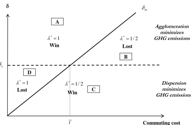
(i) The ecological viewpoint. We determine the conditions under which the market yields a good or a bad outcome from the ecological viewpoint. Because m = 0 at t = 0 and increases
with t, while e is independent of t, there are four possible cases, which are depicted in Figure
1. In panels A and C, the market outcome minimizes pollution. In contrast, in panels B and D, the market delivers a con…guration that maximizes the emissions of GHG. Consequently, the market may yield as well as the best or the worst ecological outcome.
Insert Figure 1 about here Figure 1 shows that there exists a unique t such that
m T e i¤ t T t:
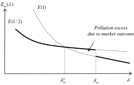
Consider …rst the case where t > t (see Figure 2a). If < m, the market outcome
involves two cities. Keeping this con…guration unchanged, a higher value of always reduces the emissions of pollutants. Note, however, that lower levels of GHG emissions could be reached under agglomeration for 2 [ e; m]. Once exceeds m, the economy gets agglomerated, thus
leading to a downward jump in the GHG emissions. Further increases in yield lower emissions of GHG. Hence, when commuting costs are high enough, denser cities generate lower emissions of GHG.
Assume now that t < t (see Figure 2b). As in the foregoing, provided that < m,
the market outcome involves dispersion while the pollution level decreases when the cities get more compact. When crosses m from below, the pollution now displays an upward jump.
Under dispersion, however, lower levels of GHG emissions would have been sustainable over [ m; e]. In other words, more compact cities need not be ecologically desirable because this
recommendation neglects the fact that it may trigger interurban migrations. Consequently, once it is recognized that workers and …rms are mobile, what matters for the total emission of GHG is the mix between the urban compactness ( ) and the interregional pattern ( ). This has the following major implication: environmental policies should focus on the urban system as a whole and not on individual cities.
Insert Figures 2a and 2b about here
The foregoing discussion shows how di¢ cult it is in practice to …nd the optimal mix of instruments. Our model also allows us to derive some unsuspected results regarding the ability of instruments other than regulating the population density (carbon tax, low emission transport technology, ...) to reduce pollution. For example, when t < t the development of more ecological technologies in shipping goods between cities (low eT) combined with the implementation of a
carbon tax on carriers, which causes higher transport costs (high ), lead to a higher value of
eand a lower value of m. This makes the interval [ m; e]wider, while the value of t increases.
Hence, the above policy mix, which seems a priori desirable, may exacerbate the discrepancy between the market outcome and the ecological optimum. Therefore, when combining di¤erent environmental policies, one must account for their impacts on the location of economic activities. Otherwise, they may result in a higher level of GHG emissions.
The conventional wisdom is that population growth is a key driver in damaging the envi-ronmental quality of cities. Restraining population growth is, therefore, often seen as a key instrument for reducing pollution. Indeed, for a given intercity pattern and a given density
level, dEm=dL > 0 because a bigger population generates larger trade ‡ows and longer
com-muting. Nevertheless, because …rms and workers are mobile, a population hike may change the intercity pattern of the economy. For that, we must study how the corresponding increase in population size a¤ects the greenness of the economy. In our setting, increasing L has the fol-lowing two consequences. First, it raises the density threshold level (d e=dL > 0) above which
agglomeration is the ecological optimum. Second, dispersion becomes the market equilibrium for a larger range of density levels (d m=dL > 0). What matters for our purpose is how the
four domains in Figure 1 are a¤ected by a population hike.
When t increases with L, then m e decreases with L provided that t > t, whereas e m
increases when t < t. In this event, urban population growth decreases the occurrence of a con‡ict between the market and the ecological objective when commuting costs are high enough (see Figure 2a) but makes bigger the domain over which the market outcome is ecologically bad (see Figure 2b). When t decreases with L, the opposite holds. In both cases, as already noted by Kahn (2006) in a di¤erent context, there is no univocal relationship between urban population growth and the level of pollution. Our analysis provides a rationale for the non-monotonicity of the relationship observed between these two magnitudes.
To sum up,
Proposition 3 Assume that cities are monocentric. If commuting costs are high, making cities more compact reduces pollution when the economy shifts from dispersion to agglomeration. However, when commuting costs are low, an increasing-density policy may be detrimental from the ecological viewpoint.
The assumption of a constant population density is very restrictive. At the same time, it is well known that characterizing the market outcome with an endogenous determination of the population density in NEG-type models is a formidable task, which has been so far out of reach (Tabuchi, 1998). We want to take an intermediate approach in which the density is variable but exogenous. More precisely, we assume that the population density is now given by f (x) where f (x) is a strictly decreasing function of the distance x to the CBD. In this case, a third spatial con…guration spatial may emerge: the market outcome and the ecological optimum may involve a large and a small monocentric city when commuting costs take on intermediate values. However, as in the case of a uniform distribution of population density, increasing leads to lower land rents, which pushes toward a more concentrated pattern of activities and a higher value of the total distance travelled by commuters. Though the analytical details become much more cumbersome, Proposition 3 remains true. An example is explicitly dealt with in Appendix B.
(ii) The welfare viewpoint. As seen in the introduction, transporting people and com-modities involves economic and ecological costs. It is not clear, however, what the welfare
implications of a higher population density are because the market outcome and the solution minimizing the ecological footprint involve di¤erent consumption levels of the manufactured good and of the numéraire. Therefore, it is important to …gure out how social welfare is a¤ected by changing the population density level.
For a given intercity distribution of activities, a higher population density is always welfare-enhancing because the average commuting costs are lower. However, when the population density becomes su¢ ciently high, …rms and workers get agglomerated. In addition to increasing urban costs, this change in the spatial pattern has two e¤ects on the utility level. First, it leads to a wage e¤ect which is ambiguous. Indeed, agglomeration triggers …ercer competition and lowers the domestic price, which tends to reduce pro…ts. Simultaneously, …rms supply all consumers at a lower cost, thus leading to an output hike which tends to increase pro…ts.6 Second, as the negative e¤ect of transport costs on consumption vanish, the consumer surplus increases (12). The total impact of denser cities on social welfare is, therefore, unclear. As a consequence, we must assess how the socially optimum con…guration is a¤ected by a higher population density. Because we study the environmental gains or losses associated with the market outcome, we …nd it natural to adopt a second-best approach in which the planner controls the location of …rms and workers but not their production and consumption decisions. Because utilities are quasi-linear and pro…ts are wiped out by free entry, social welfare may be de…ned by the sum of indirect utilities evaluated at the equilibrium prices and incomes. In what follows, we have chosen to focus on welfare without accounting for the negative impact of pollution because weighting this externality in the social welfare function is often arbitrary. For the same reason, we do not include the various impacts that a higher population density has on the well-being of people.
Plugging the equilibrium values of Sr, wr and U Crinto (11) for a given intercity distribution
of …rms and workers, the welfare function is given by
Wm( ) = LS1 + (1 ) LS2 + L(w1 U C1) + (1 ) L(w2 U C2) (17) = L(" o a "ob ) ( 1) ( o) + (L + 2) L 2(L + 1)2 tL 2 where o t ("o a "ob ) > m
and "oa 2 (L + 2) =(L + 1)2 and "ob (2L2 + 5L + 4)=2(L + 1)2. Hence, agglomeration
(dispersion) is welfare-maximizing when > o ( < o). The formal connection between
the external environmental cost E and the social welfare function Wm is now clear: both are
second-order polynomials in and the density governs the sign of their second derivatives. Let o be the intercity distribution maximizing Wm. The individual utilities being
quasi-linear, interpersonal transfers allow consumers to reach their optimum utility level W ( o)=L,
6It is readily veri…ed that q
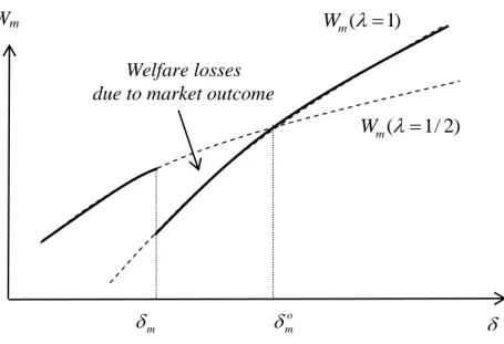
which is larger than the equilibrium utility level V ( ). As a consequence, the market yields agglomeration when o > > m, whereas dispersion is socially desirable. Otherwise, the
market outcome and the social optimum are identical. However, this does not mean that a higher density is always welfare-enhancing. For example, as shown by Figure 3, when crosses
m from below, the welfare level displays a downward jump.
Insert Figure 3 about here
Observe that both the social welfare Wm and the carbon footprint E are second-degree
polynomials in . In addition, the density governs the sign of their second derivatives. As a a result, social welfare and the amount of pollutants may be convex or concave functions of meaning that making cities more compact may or may not increase welfare and/or decrease pollution. Since o exceeds m, two cases may arise:
(i) When commuting costs are low (t < t), our results imply that an increasing-population density policy should be accompanied by a growth control policy. Indeed, the polluting emis-sions in the global economy increases when crosses m from below and takes a value in
[ m; o] (see Figure 2b). In this case, by preventing the agglomeration of activities, the public
authorities both reduce the GHG emissions and improve global welfare.
(ii) When commuting costs are high (t > t), the desirability of a growth control policy is more controversial. When crosses m from below and takes a value in [ m; o], such a policy
yields higher welfare but washes out the environmental gains generated by the market (see Figure 2a). This is not, however, the end of the story. The con‡ict between the environmental and welfare criteria vanishes when > o because the market outcome both minimizes GHG
emissions and maximizes social welfare. To summarize,
Proposition 4 Assume that cities are monocentric. If commuting costs are low, a higher population density may be harmful to both the environment and social welfare when the economy switches from dispersion to agglomeration. If commuting costs are high, a higher population density reduces pollution but may generate a welfare loss.
This proposition is su¢ cient to show that the desirability of compact cities is more complex than suggested by their proponents, the main reason being that this recommendation disregards its impact on the location of economic activity.
4
The urban system and the environment
So far, we have treated the morphology of cities as given. In this section, we provide the ecological and welfare evaluation of the market outcome when the size and structure of each
city are endogenously determined. To reach our goal, we build on Cavailhès et al. (2007). Having done this, we show once more the possible perverse e¤ects of city compactness and highlight the positive e¤ects of job decentralization. Speci…cally, we argue that an alternative strategy could reduce the pollution emissions in the global economy: public authorities control the intra-urban distribution of …rms and workers to decrease the average distance traveled by workers.
4.1
The size and structure of cities
In what follows, we determine the conditions for a city to become polycentric and, then, study how raising population density shapes the urban system.
1. The city structure. Firms are free to locate in the CBD or to form a secondary business district (SBD) on each side of the CBD, thus implying that a polycentric city has one CBD and two SBDs. Both the CBD and the SBDs are surrounded by residential areas occupied by workers. Although …rms consume services supplied in the SBD, the higher-order functions (speci…c local public goods and non-tradeable business-to-business services) are still provided by the CBD. Hence, for using such services, …rms established in a SBD must incur a communication cost K > 0. Communicating requires the acquisition of speci…c facilities, which explains why communication costs have a …xed component. Furthermore, as the distance between the CBD and SBDs is small compared to the intercity distance, shipping the manufactured good between the CBD and SBDs is assumed to be costless, which implies that the price of this good is the same everywhere within a city. Finally, without signi…cant loss of generality, we restrict ourselves to the case of two SBDs. Hence, apart from the assumed existence of the CBD, the internal structure of each city is endogenous. Note that the equilibrium distribution of workers within cities depends on the distribution of workers between cities. In what follows, the superscript c is used to describe variables related to the CBD, whereas s describes the variables associated with a SBD.
At a city equilibrium, each worker maximizes her utility subject to her budget constraint, each …rm maximizes its pro…ts, and markets clear. Individuals choose their workplace (CBD or SBD) and their residential location for given wages and land rents. Given equilibrium wages and the location of workers, …rms choose to locate either in the CBD or in a SBD. Or, to put it di¤erently, no …rm has an incentive to change place within the city, and no worker wants to change her working place and residence. In particular, at the city equilibrium, the distribution of workers is such that Vrc( ) = Vrs( ) Vr( ). Likewise, …rms are distributed at the city
equilibrium such that c
r( ) = sr( ).
Denote by yr the right endpoint of the area formed by residents working in the CBD and
also the outer limit of city r. Let xs
r be the center of the SBD in city r. Therefore, the critical
points for city r are as follows: yr= rLr 2 x s r = (1 + r) Lr 4 zr= Lr 2 (18)
where r < 1 is the share of city r-…rms located in the CBD. Observe that the bid rents at yr
and zr are equal to zero because the lot size is …xed and the opportunity cost of land is zero.
At the city equilibrium, the budget constraint implies that
wcr Rcr(x)= tx = wrs Rrs(x)= tjx xsrj
where Rcr and Rsr denote the land rent around the CBD and the SBD, respectively. Moreover,
the worker living at yr is indi¤erent between working in the CBD or in the SBD, which implies
wrc Rcr(yr)= tyr = wrs R s
r(yr)= t(xsr yr):
It then follows from Rcr(yr) = Rsr(yr) = 0 that
wcr wrs= t(2yr xsr) = t
3 r 1
4 Lr (19)
where we have used the expressions of yr and xsr given in (18).
In each workplace (CBD or SBD), the equilibrium wages are determined by the zero-pro…t condition. As a result, the equilibrium wage rates in the CBD and in the SBD must satisfy the conditions c
r(wcr; wsr) = sr(wcr; wsr) = 0. Solving these expressions for wcr and wrs, we get:
wrc = r wsr = r K (20)
which shows that the wage wedge wc
r wsr is positive.
Finally, the equilibrium land rent in the area occupied by the CBD-workers is given by Rr(x) = Rcr(x) = t
rLr
2 x for x < yr (21)
where we have used the expression of yr and the condition RC(yr) = 0, while the equilibrium
land rent in the area occupied by the SBD-workers is as follows:7 Rr(x) = Rrs(x) = t
(1 r) Lr
4 + x
s
r x for xsr < x < zr: (22)
Substituting (10) and (20) into (19) and solving with respect to yields:
r = min 1 3 + 4 K 3tLr ; 1 (23)
7In this expression, we do not account for the fact that transport modes may not be the same in these
di¤erent areas of the metropolis. Our results remain valid as long as individual worktrips to a SBD do not generate much higher pollutants than those to the CBD.
which always exceeds 1=3: the CBD is always larger than each SBD. It is readily veri…ed that city r is polycentric ( r < 1) if and only if
< r
tLr
2K: (24)
Observe also that, when r < 1, a larger population Lr leads to a decrease in the relative
size of the CBD, though its absolute size rises, whereas both the relative and absolute sizes of the SBDs rise. Indeed, increasing rLleads to a more than proportionate hike in the wage rate
prevailing in the CBD because of the rise in the average commuting cost (see (19)). Moreover, because r < 1, the higher the city compactness, the larger the CBD; the lower the commuting
cost, the larger the CBD. In short, when city compactness steadily rises, both SBDs shrink smoothly and, eventually, the city becomes monocentric.
2. The urban system. The utility di¤erential between cities now depends on the degree of job decentralization within each city. The indirect utility of an individual working in the CBD is still given by (11) in which the urban costs she bears are now given by8
U Crc rtLr
2 < U Cr: It follows from (24) that
1
Lt
2K 2
(1 )Lt
2K (25)
where 1 2 because we focus on the domain 1=2. The following three patterns may
emerge: (i) when > 1, both cities are monocentric ( 1 = 2 = 1), (ii) when 1 > > 2,
city 1 is polycentric and city 2 is monocentric ( 1 < 2 = 1) (iii) when 2 > , both cities are
polycentric ( r < 1).
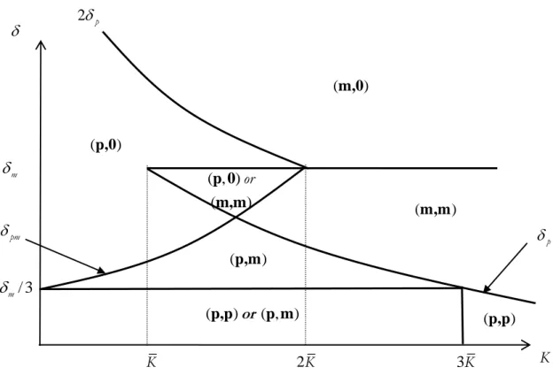
In order to determine the equilibrium outcome, we must consider the utility di¤erential cor-responding to each of these three patterns. In Appendix D, we show the existence and stability of …ve equilibrium con…gurations: (i) dispersion with two monocentric cities having the same size (m; m); (ii) agglomeration within a single monocentric city (m; 0);(iii) partial agglomera-tion with one large polycentric city and a small monocentric city (p; m); (iv) agglomeraagglomera-tion within a single polycentric city (p; 0) and (v) dispersion with two polycentric cities having the same size (p; p): In Figure 4, the domains of the positive quadrant (K; ) in which each of these con…gurations is a market outcome are depicted.
Insert Figure 4 about here
The implications of city compactness depend on the level of communication costs. We focus here on the today relevant case of low communication costs (see Appendix D), i.e.
K < K L("a "b )
4 :
8We may disregard the case of SBD-workers because, at the city equilibrium, they reach the same utility
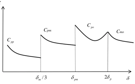
In this event, the economy traces out the following path when the population density steadily increases from very small to very large values: we have (p; p) or (p; m) when < m=3, then
(p; m) when m=3 < < pm, further (p; 0) when pm < < 2 p with p Lt=4K (see
Appendix D for more details) and (m; 0) when 2 p < , with pm
t
3("a "b ) 4K=L
which is positive because K < K. This may be explained as follows. By inducing high urban costs, a low -value leads to both the dispersion and decentralization of jobs, that is, the emergence of two polycentric cities. When cities’ population density gets higher, urban costs decrease su¢ ciently for the centralization of jobs within one city to become the equilibrium outcome; however, they remain high enough for the equilibrium to involve two cities of di¤erent sizes and structures. Last, for very high -values, urban costs become almost negligible, thus allowing one to save the cost of shipping the manufactured good through the emergence of a single city.
4.2
How the structure and size of cities impact on the environment?
We now determine whether more compact cities lead to lower GHG emissions when …rms and workers are free to locate between and within cities.
The total level of emissions of GHG corresponding to the spatial structure ( ; 1; 2) is given by
E( ; 1; 2) = eCC( ; 1; 2) + eTT ( ):
Note …rst that the value of T is still given by (15) because it does not depend on the city structure. In contrast, the total distance travelled by commuters depends on the internal structure of each city ( 1 and 2) as well as on the distribution of workers/…rms between cities:
C( ; 1; 2) = 2L2 4 2 1+ 1 2(1 1) 2 +(1 )2L2 4 2 2+ 1 2(1 2) 2 (26)
which boils down to (14) when the two cities are monocentric ( 1 = 2 = 1). It is straightforward
to check that the GHG emissions increase when the CBDs grow. However, the strength of this e¤ect decreases when cities become more compact.
For any given , the expression (26) shows that the decentralization of jobs away from the CBD leads to less GHG emissions through a shorter average commuting. Regarding the impact of a higher population density, it is a priori ambiguous. Indeed, for a given degree of job decentralization, a higher population density induces shorter commuting distances and, therefore, lower emissions. However, (23) shows that a rising also leads to a higher number of jobs in the CBD at the expense of the SBDs, which increases the emission of GHG. Plugging (23) into (26), we readily verify that the former e¤ect dominates the latter. Thus, for any given , more compact cities always generate lower GHG emissions once the city equilibrium is reached. However, this result may be reverse once workers/…rms can relocate between cities.
(i) Commuting. In order to disentangle the various e¤ects at work, we begin by focusing on pollution stemming from commuting. For any given location pattern, a higher leads to a lower level of pollution. However, the impact of such a change in population density on the total distance travelled by commuters is not clear when …rms and workers may change places within and between cities. In addition, one may wonder what happens when the economy shifts from one pattern to another.
To illustrate, we assume that the initial market outcome is given by (p; p). The correspond-ing GHG emissions generated by commutcorrespond-ing are then given by
Cpp
L2
24 2 + 4K2
3t2 :
As long as this urban con…guration prevails, a higher population density reduces commuting pollution.9 However, once crosses m=3from below, the economy shifts to the con…guration
(p; m) (see Figure 4). At = m=3, the level of pollution exhibits an upward jump.10 This is
because city 1, which remains polycentric, becomes larger while city 2, which now accommodates fewer workers, becomes monocentric.
At the equilibrium con…guration (p; m), pm increases with whenever K < K.11 In this
case, (23) and (26) show that the level of pollution Cpm unambiguously decreases with .
However, at = pm, the economy moves from (p; m) to (p; 0), which implies that the level of
GHG emissions due to commuting is given by Cpo =
L2
12 2 + 2K2
3t2 :
Once more, a change in the intercity structure generates an upward jump in commuting pollution.12
When keeps rising, the CBD grows at the expense of the SBDs. Under these circum-stances, Cpo decreases for <
p
2 p but increases when rises from
p
2 p to 2 p. Because jobs
relocate in the CBD at the expense of the SBDs in response to higher population density, the average distance traveled by commuters may increase. This result might come as something of a surprise because it says that making a polycentric city more compact need not be good for the environment, even when the city remains polycentric. We are thus far from the famous “compact is always better.”
Finally, when reaches the threshold 2 p, the SBDs vanish, meaning that city 1 becomes
monocentric. At = 2 p, we have Cpo = Cmo where
Cmo= L2 4 : 9Indeed, dC pp=d < 0 if and only if p= p 2. Because p= p 2 > m=3 when K < K, we have dCpp=d < 0
as long as the economy involves two identical polycentric cities ( < m=3). 10Indeed, we have C
pp < Cpm when m=3. 11The value of
pm can be determined from case (iii) in the Appendix B by solving pmV ( ) = 0. 12This is because C
In this case, increasing further the population density leads to lower pollution.
The entire equilibrium path is described in Figure 5. It reveals an interesting and new result: although increasing the population density is likely to reduce GHG emissions when the city size remains unchanged, the resulting change in urban structure might well raise the GHG emissions stemming from commuting. In particular, because the minimum value of Cpm over
( m=3; pm) exceeds the maximum value of Cpp over ( p; m=3), moving from (p; p) to (p; 0)
through (p; m) leads to higher levels of commuting pollution. In other words, by a¤ecting the urban system, a higher population density may have undesirable e¤ects from the environmental viewpoint.
Insert Figure 5 about here
(ii) Shipping. Consider now GHG emissions generated by the transport of goods. Dis-persion ( = 1=2) is the worst and agglomeration ( = 1) the best con…guration: T (1=2) > T ( pm) > T (1). Consequently, for K < K, the recommendations based on commuting (C) and interregional shipping (T ) do not point to the same direction. Speci…cally, when the city structure shifts from (p,m) to (p,0), the pollution generated by workers’commuting jumps up-ward, whereas the pollution stemming from shipping goods vanishes. In this event, it is a priori impossible to compare the various market outcomes, hence to determine the best ecological con…guration. Yet, given the relative importance of commuting and other within-city trips in the global emission of carbon dioxides, we believe that the conclusions derived for the former case are empirically relevant.
4.3
Welfare and the environment
The above results suggest that the decentralization of jobs within cities should supplement a higher population density from the ecological standpoint. One may wonder what this recom-mendation becomes when it is evaluated at the light of a second-best approach in which the planner chooses the number and structure of cities ( o; o1; o2).
At any given intercity distribution of …rms ( ), the intra-urban allocation of …rms maximiz-ing global welfare is given by:
o r = 1 3 + 2 K 3tLr < r: (27)
Hence, starting from the market equilibrium ( r), a coordinated decentralization of jobs within
cities both raises welfare and decreases GHG emissions. It is readily veri…ed that socially optimal outcome implies that city r is polycentric if
< or tLr
K : (28)
Let us now turn to the case where the intercity distribution of activities and the city structure are both endogenous. As in the foregoing, we restrict ourselves to the case of low communication
costs (K < K). It is shown in Appendix E that the welfare optimum is given by (i) two identical polycentric cities when o=3 > , (ii) two asymmetric cities when opm > > o=3,
(iii) one single polycentric city when 4 p > > opm, and (iv) one single monocentric when
> 4 p (the expression of opm is given in Appendix E). Because o > m and opm > pm,
the market need not deliver the optimal con…guration. For example, the market sustains two asymmetric cities when o=3 > > m=3while the second-best optimum involves two identical
polycentric cities. In addition, when opm> > o=3, a single polycentric city is the equilibrium
spatial con…guration; the second-best optimum is given by a large polycentric city with a small monocentric city.
Consequently, as in Section 3, when …rms and workers’ locations are given, a marginal increase in is always ecologically and socially desirable. However, when the population density hike generates a new pattern of activities, the move may be detrimental to both objectives. For instance, when crosses m=3from below and takes a value in [ m=3; o=3], pollution from
commuting exhibits an upward jump (see Figure 5). Moreover, the market outcome involves two asymmetric cities (p,m), while the second-best optimum involves two identical polycentric cities. This shows that what we have seen in Section 3 remains valid when the morphology of the urban system is endogenous. Though incomplete, our analysis suggests that there is no systematic con‡ict between welfare and environmental objectives.
5
Conclusion
This paper has focused on a single facet of compact cities: the transport demand. Observe, however, that trips related to activities such as recreation and schooling have a less direct rela-tion to the city structure than commuting, thus blurring the connecrela-tion between compactness and GHG emissions. Our model, therefore, should be extended to account for the location of such facilities. Furthermore, we have left aside the role of population density in the emissions of carbon dioxides generated by home heating and air conditioning. For example, residential energy use accounts for another 20% of America’s GHG emissions. Therefore, a housing sector should be grafted onto our setting to capture this additional facet of the problem. In the same vein, it should be recognized that high population densities generate congestion and other neg-ative externalities that are likely to clash with the social norms prevailing in many developed countries. Another limit of our approach is the implicit assumption of “liquid housing”in that the population density may be increased at no cost. Accounting for adjustment costs in housing size would make the case for compact cities weaker. Finally, our planning approach should be compared to a decentralized mechanism in which cities are free to choose their land-use policies. Due to the lack of coordination between jurisdictions, one may expect more tension to occur
between the ecological and social welfare objectives.13
To sum up, our work is too preliminary for strong and speci…c policy recommendations. This work must be viewed as a …rst step toward a theory of an ecologically and socially desirable urban system. We believe, however, that our results are su¢ ciently convincing to encourage city planners and policy-makers alike to pay more attention to the various implications of urban compactness. Unless modal changes lead workers to use mass transport systems, compact and monocentric cities may generate more pollution than an urban system with polycentric dispersed cities. In addition, by lowering urban costs without reducing markedly the bene…ts generated by large urban agglomerations, the creation of secondary business centers may allow large cities to reduce GHG emissions while enjoying agglomeration economies. The future of China and India, among others, will be urban, and the land-use rules they choose will have a considerable impact on the world carbon footprint (Glaeser, 2011). Building tall cities is clearly part of the answer, but we contend that policy-makers should also pay attention to the structure and number of the megacities that will emerge.
References
[1] A. Bento, S. Franco, D. Ka¢ ne, The e¢ ciency and distributional impacts of alternative anti-sprawl policies, Journal of Urban Economics 59 (2006) 121-141.
[2] J. Brander, P. R. Krugman, A “reciprocal dumping”model of international trade, Journal of International Economics 15 (1983) 313-321.
[3] D. Brownstone, T. Golob, The impact of residential density on vehicle usage and energy consumption, Journal of Urban Economics 65 (2009) 91-98.
[4] J. K. Brueckner, Urban sprawl: Diagnosis and remedies, International Regional Science Review 23 (2000) 160-171.
[5] J. Cavailhès, C. Gaigné, T. Tabuchi, and J.-F. Thisse, Trade and the structure of cities, Journal of Urban Economics 62 (2007) 383-404.
[6] B. Copeland, S. Taylor, Trade and the Environment: Theory and Evidence, Princeton Univ. Press, Princeton, 2003.
[7] G.B. Dantzig, T.L Saaty, Compact city. A plan for a liveable urban environment, W.H. Freeman, San Francisco, 1973.
13In particular, as observed by Glaeser and Kahn (2010), more empirical work is needed to determine whether
[8] G. Duranton, D. Puga, Micro-foundations of urban increasing returns: theory, in J.V. Henderson and J.-F. Thisse (Eds.), Handbook of Regional and Urban Economics. Volume 4, North Holland, Amsterdam, 2004, pp. 2063-117.
[9] C. Engel, J. Rogers, How wide is the border? American Economic Review 86 (1996) 1112–1125.
[10] C. Engel, J. Rogers, Deviations from purchasing power parity: Causes and welfare costs, Journal of International Economics 55 (2001) 29–57.
[11] European Environment Agency, Greenhouse gas emission trends and projections in Europe 2007. European Environment Agency Report No 5, COPOCE, European Union, 2007. [12] Environmental Protection Agency, US Greenhouse Gas Inventory Report, 2011.
[13] Gaigné C., S. Riou and J.-F. Thisse, Are compact cities environmentally friendly? Discus-sion Paper N 8297, CEPR, 2011.
[14] C. Gaigné, I. Wooton, The gains from preferential tax regimes reconsidered, Regional Science and Urban Economics 41 (2011) 59-66.
[15] E.L. Glaeser, Triumph of the City, Macmillan, London, 2011.
[16] E.L. Glaeser, M.E. Kahn, Sprawl and urban growth, in J.V. Henderson and J.-F. Thisse (Eds.), Handbook of Regional and Urban Economics. Volume 4, North Holland, Amster-dam, 2004, pp. 2481-527.
[17] E.L. Glaeser, M.E. Kahn, The greenness of cities: carbon dioxide emissions and urban development, Journal of Urban Economics 67 (2010) 404-418.
[18] P. Gordon, H.W. Richardson, Are compact cities a desirable planning goal? Journal of the American Planning Association 63 (1997) 1-12.
[19] A. Hau‡er, I. Wooton, Competition for …rms in an oligopolistic industry: The impact of economic integration, Journal of International Economics 80 (2010) 239-248.
[20] Kahn, M.E., Green Cities: Urban Growth and the Environment, Brookings Institution Press, Washington, DC, 2006.
[21] M.E Kahn, J. Schwartz, Urban air pollution progress despite sprawl: the “greening”of the vehicle ‡eet, Journal of Urban Economics 63 (2008) 775-787.
[22] I. Muniz, A. Galindo, Urban form and the ecological footprint of commuting. The case of Barcelona, Ecological Economics 55 (2005) 499-514.
[23] OECD, Highlights of the international transport forum 2008: transport and energy. The challenge of climate change. OECD Publishing, Paris, 2008.
[24] G.I.P. Ottaviano, T. Tabuchi, J.-F. Thisse, Agglomeration and trade revisited, Interna-tional Economic Review 43 (2002) 409-436.
[25] J.M. Savin, L’évolution des distances moyennes de transport des marchandises. Note de synthèse du SES, Logistique, May-June 2000.
[26] L. Schipper, L. Fulton, Carbon dioxide emissions from transportation: Trends, driving forces and forces for change, in D.A. Hensher and K.J. Button (Eds.), Handbook of Trans-port and the Environment, Elsevier, Amsterdam, 2003, pp. 203-226.
[27] N. Stern, The economics of climate change, American Economic Review 98 (2002) 1-37. [28] T. Tabuchi, Agglomeration and dispersion: A synthesis of Alonso and Krugman, Journal
of Urban Economics 44 (1998) 333-51.
[29] D. Timothy, W. Wheaton, Intra-urban wage variation, employment location, and com-muting times, Journal of Urban Economics 50 (2001) 338-366.
[30] J.-F. Thisse, Toward a uni…ed theory of economic geography and urban economics, Golden Issue of Journal of Regional Science 50 (2010) 281-296.
[31] US Census Bureau, US Commodity ‡ow survey, 2007.
6
Appendix A
Accounting for emissions stemming from shopping-trips and manufacturing production do not change the qualitative properties of our fundamental trade-o¤.
- If shopping malls, say, are located at the city outskirts, this means that a consumer located at x has to travel the distance yr x = Lr=2 xto go to the mall. If the number of shopping
trips is given by > 0, C( ) must be supplemented by M ( ) = 2 Z y1 0 (y1 x)dx + 2 Z y2 0 (y2 x)dx = C( )
and thus C( ) + M ( ) = ( + 1)C( ). As a result, accounting for shopping trips in (13) amounts to giving a higher weight to the component capturing the within-city emissions. Of course, this argument does not account for localized trips, such as those made to schools. As shown by Glaeser and Kahn, the length of these trips also depends on the density. Their total length decreases with but increases with , very much like C.
- The carbon footprint E of the urban system can be augmented by introducing emissions stemming from production. The total output is given by
Q1( ) + Q2( ) = L
2
L + 1[1 2 (1 )]:
Thus, production behaves like C and is minimized (maximized) when = 1=2 ( = 1). It suggests that accounting for production in the carbon footprint of cities makes the case for dispersion stronger.
Appendix B
To see how things work, assume that f (x) = 1 kx with k < =L (hence, regardless the city size, we have 1 kyr > 0). The meaning of is as before while a low value of k means that the
distribution is dispersed; it is uniform when k = 0. The right endpoint of city r is now such that
Z yr
0
(1 kx)dx = Lr 2 the solution of which is
yr =
1 p1 kLr=
k :
It is readily veri…ed that dyr=dLr > 0and d2yr=dL2r > 0as well as dyr=d < 0 and dyr=dk > 0.
In other words, the spatial extension of city r increases with its population size and decreases with its population density, that is, a higher and a smaller k. Note also that yr = Lr=2 when
k = 0.
The urban costs are now given by U Cr =
t k 1
p
1 kLr=
while the equilibrium wages and surplus are not a¤ected by k. Standard calculations show that full agglomeration arises if and only if
m <
kL
2 1 p1 kL= A and full dispersion if and only if
m >
r
1 kL
2 D:
Note that D = A = when k = 0. In addition, since k < =L we have D > A. As a
consequence, we have full dispersion when < Dm where Dm is the solution to D( ) = m with D
m = max kL +
q
k2L2+ 16 2
partial agglomeration when Am > > Dm where Am is the solution to A( ) = m with A
m = 4 2
m=(4 m kL);
and full agglomeration when > Am. It is straightforward to check that Am = Dm = m when
k = 0. In addition, we have Am = Dm = 0 when t = 0 and Am ! 1 and Dm ! 1 when t ! 1. In the case of partial agglomeration, the spatial equilibrium is given by
= 1 2 + 2 m p D m L k : The sum of distance traveled by workers is now given by
C( ) = 2X r Z yr 0 x( kx)dx = 1 2 kyr 3 y 2 r:
This function reaches its minimum at = 1=2 while C( ) = L2
r=4 when k = 0. It is
straight-forward to check that E is minimized at
e = 1 2 + eC eT p Y kLZ where Y 1 Lk 2 e2 C 4e2 T 2Z2 Z [2 (L + 2)]=(L + 1):
It is readily veri…ed that e = 1=2 ( e = 1) if and only if is su¢ ciently small (large), whereas e belongs to the interval (1=2; 1) for intermediate values of . Consequently, the positive quadrant of the (t; )-space is now divided into several domains in which the market delivers either a good or a bad ecological outcome, very much as in the case of uniform densities. This is illustrated in Figure 1b where the market outcome minimizes pollution in Panels A and C while in panels B’, D’and E, the market delivers a bad ecological outcome.
Figure 1b
Appendix C
When cities can be monocentric or polycentric, the welfare function becomes
W ( 1; 2; ) = LS1 + L2S2 + 1 L(wC1 U C C 1 ) + 2(1 ) L(w2C U C C 2 ) + (1 1) L(w1S U C S 1) + (1 2) (1 ) L w2S U C S 2 :
Plugging (27) into this expression, we get the following cases.
(i) If > o1 where o1 is given by (28), both cities must be monocentric and the social optimum is given by the maximizer of (17).