VARIATION SPA TIO-TEMPORELLE DE LA MACROF AUNE ENDOBENTHIQUE DANS LA ZONE PROFONDE DU SAINT -LAURENT (QUÉBEC, CANADA) EN
RELATION AVEC LES CONDITIONS ENVIRONNEMENTALES
MÉMOIRE PRÉSENTÉ À
L'UNIVERSITÉ DU QUÉBEC À RIMOUSKI comme exigence partielle
du programme de maîtrise en océanographie
PAR
MYLÈNE BOURQUE
Avertissement
La diffusion de ce mémoire ou de cette thèse se fait dans le respect des droits de son auteur, qui a signé le formulaire « Autorisation de reproduire et de diffuser un rapport, un mémoire ou une thèse ». En signant ce formulaire, l’auteur concède à l’Université du Québec à Rimouski une licence non exclusive d’utilisation et de publication de la totalité ou d’une partie importante de son travail de recherche pour des fins pédagogiques et non commerciales. Plus précisément, l’auteur autorise l’Université du Québec à Rimouski à reproduire, diffuser, prêter, distribuer ou vendre des copies de son travail de recherche à des fins non commerciales sur quelque support que ce soit, y compris l’Internet. Cette licence et cette autorisation n’entraînent pas une renonciation de la part de l’auteur à ses droits moraux ni à ses droits de propriété intellectuelle. Sauf entente contraire, l’auteur conserve la liberté de diffuser et de commercialiser ou non ce travail dont il possède un exemplaire.
RÉSUMÉ
L'estuaire maritime et le golfe du Saint-Laurent fonnent un système complexe où la dynamique des conditions environnementales détennine les variations spatiales et temporelles au niveau des communautés benthiques. L'observation récente de zones hypoxiques profondes dans l'estuaire maritime du Saint-Laurent pourrait avoir une influence majeure sur la structure de ces communautés, étroitement liées aux conditions environnementales. Toutefois, la macro faune benthique du Saint-Laurent reste encore méconnue. Afin de définir un éventuel impact sur l'aspect fonctionnel des communautés, la structure de la macrofaune benthique a été caractérisée dans le but de voir si les zones hypoxiques se traduisent par des modifications des communautés.
Notre objectif était de décrire les patrons de distribution des communautés endobenthiques dans deux régions du Saint-Laurent, l'estuaire maritime et le golfe du Saint-Laurent, et d'identifier les facteurs environnementaux influençant la structure des communautés. De plus, les variations temporelles au niveau des caractéristiques des communautés ont été décrites, afin de détenniner les effets potentiels de l'hypoxie. La macrofaune endobenthique a été échantillonnée en 2005 et 2006 à 20 stations, réparties le long de la zone profonde des deux régions étudiées. Les données ont été analysées selon une approche univariée et multivariée. Sept groupes de stations, basés sur l'abondance taxonomique, ont été identifiés dans la zone d'étude, selon une analyse par groupement. Les résultats ont montré une grande variabilité spatiale de la répartition des assemblages benthiques et des groupes fonctionnels, ainsi que des indices de diversité. La composition du sédiment (taille moyenne des grains et matière organique), la température et la salinité sont panni les facteurs environnementaux influençant les assemblages d'espèces et les groupes fonctionnels. Les indices de diversité sont plutôt influencés par la profondeur, l'oxygène, la température et la taille du sédiment. L'analyse des données historiques démontre une diminution temporelle de la richesse spécifique et de la diversité de Shannon, attribuée possiblement au développement de l'hypoxie dans l'estuaire maritime du Saint-Laurent. Des changements au niveau des communautés benthiques ont été détectés, dont une augmentation de la densité de quelques espèces opportunistes vivant à la surface du sédiment, tels les polychètes du genre Myriochele, généralement présentes dans les premières étapes d'un milieu perturbé par l'hypoxie. Dans un contexte de changements climatiques, ces travaux pennettront de mieux comprendre les causes et les impacts écologiques de l 'hypoxie afin de déterminer les effets potentiels des modifications de la structure des communautés sur le fonctionnement global de l'écosystème.
TABLE DES MATIÈRES
RÉSUMÉ ... 1I
TABLE DES MATIÈRES ... .111
LISTE DES TABLEAUX ... v
LISTE DES FIGURES ... VII LISTE DES ANNEXES ... IX REMERCIEMENTS ... X INTRODUCTION GÉNÉRALE ... 1
CHAPITRE 1: SPATlO-TEMPORAL VARIATION IN BENTHIC MACROFAUNE AND RELATlONSHIPS WITH ENVIRO MENTAL VARIABLES IN THE DEEP ESTUARY AND GULF OF ST. LAWRENCE (QUEBEC, CANADA) ... 11
1.1 Introduction ... 12
1.2 Material and methods ... 16
1.2.1 Study area ... 16
1.2.2 Field sampling methods and 1aboratory analyses ... 17
1.2.3 Temporal historical data ... 19
1.2.4 Data analyses ... 22
1.3 Results ... 25
1.3.1 Spatial structure ofmacrobenthic infaunal communities ... 25
1.3.2 Relationships between macrobenthic community structure and environmenta1 factors ... 35
1.3.3 Temporal variability of macrobenthic communities structure ... .42
1.4 Discussion ... 51
1.4.1 Spatial distribution ofmacrobenthic assemblages ... 51
1.4.2 Spatial variability ofbenthic diversity ... 55
1.4.3 Influence of environmental variables on macrobenthic communities structure .. 57
1.4.4 Temporal variability in benthic assemblages and diversity ... 60
1.5 Conclusion ... 63
CONCLUSION GÉNÉRALE ... 65
RÉFÉRENCES ... 70
1.3.3 Temporal variability of macrobenthic communities structure ... .42
1.4 Discussion ... 51 1.4.1 Spatial distribution of macrobenthic assemblages ... 51 1.4.2 Spatial variability ofbenthic diversity ... 55
1.4.3 Influence of environmental variables on macrobenthic communities structure .. 57 1.4.4 Temporal variability in benthic assemblages and diversity ... 60
1.5 Conclusion ... 63 CONCLUSION GÉNÉRALE ... 65 RÉFÉRENCES ... 70
LISTE DES TABLEAUX
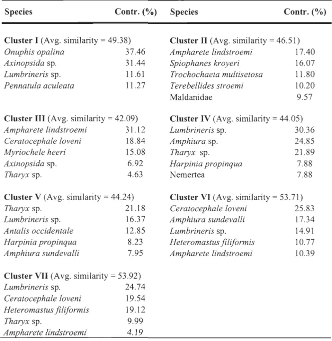
Table 1. Results of SIMPER analyses showing the contribution (%) of the five taxa (Species level) that contribute the most to the average Bray-Curtis similarity, based on
..J
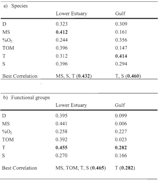
transformed densities, of compared replicates within each cluster (1 to VII) as well as the average similarity (%) for each group ofsamples ... 30 Table 2. Summary of results from BIO-ENV analyses for the Lower St. Lawrence Estuary and the Gulf of St. Lawrence, according to a) species and b) functional groups. Spearman rank correlations (rs) between biotic and abiotic similarity matrices, with highest correlations in boldo Biotic data were..J
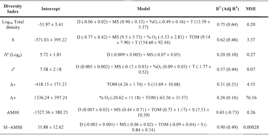
transformed; abiotic matrice constructed using Euclidean distances. Depth (D, m), mean grain size (MS, !lm), bottom oxygen saturation (%02, %), total organic matter content in the sediment(TOM, %), bottom temperature (T, OC), and bottom salinity (S, PSU) were the environmental variables used in the analysis ... 39 Table 3. Results of linear regression analyses for the a) LSLE and b) GSL, estimating total density (LOglO ind. m-2), species richness (S), diversity (H', loge), evenness (J':
H '/log sol), average taxonomic distinctness (L1 +) and variation in taxonomic distinctness (A +) among stations in a) the LSLE and b) ,the GSL. Depth (D, m), bottom temperature (T, OC), % of oxygen saturation (%02, %), mean grain size (MS, !lm) and % of total organic matter in the sediment (TOM, %) were environmentaI variables in regression models. Regression coefficients ± Standard error; total R2 (and adjusted R2
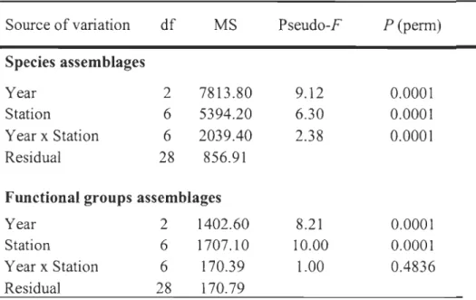
); MSE: Mean squared errors ... 40 Table 4. Permutational analysis of variance (PERMANOV A) results testing the effect of year, station and their interactions on species and functional groups assemblages based on the Bray-Curtis similarity matrices. Data were
..J
transformed prior to analysis ... 44 Table 5. Results ofSIMPER analyses showing the contribution (%) of the five taxa (Genus level) and functional groups that contribute the most to a) the average Bray-Curtis similarity of compared replicates within a year (1980 and 2005-06) as well as the average similarity (%) for each year and b) average Bray-Curtis dissimilarity of compared replicates between years (1980 and 2005-06) as well as the average dissimilarity (%), based on ..J transformed densities ... .47 Table 6. Results oftwo-way ANOVAs, showing effects of sampling year (1980 and2005-06), station and their interactions on total density (ind. m-2), species richness (S), Shannon-Wiener's diversity (H'), Pielou's evenness (J'), average taxonomie
distinetness (L1 +) and variation in taxonomie distinetness (A +). Total density was loglO transfonned ... 49
LISTE DES FIGURES
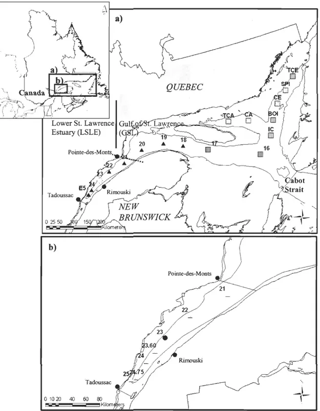
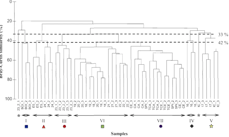
Figure 1. Schéma de la succession faunique et de la structure du sédiment le long d'un gradient d'enrichissement en matière organique (tiré de Pearson and Rosenberg, 1978) ... 8 Figure 2. a) Study area showing the location of the 17 sampling stations in 2005 (Â) and 2006 (0), with infauna and environmental data, and the deep channels. Station 23 was sampled both in 2005 and 2006 (0). b) Map of the St. Lawrence estuary showing the locations of the seven stations with infauna historical data, sampled in 1980 and 2005 (.&), except for station 23 which was sampled also in 2006 (e) ...... 21 Figure 3. a) Hierarchical clustering with group-average linking of '; transformed densities
for each replicate, using Bray-Curtis sirnilarity (%). The grouping of stations corresponded to the horizontal hnes at 33 % similarity level (1 to V) and 42 % similarity level (VI and VII).
* represent unclassified
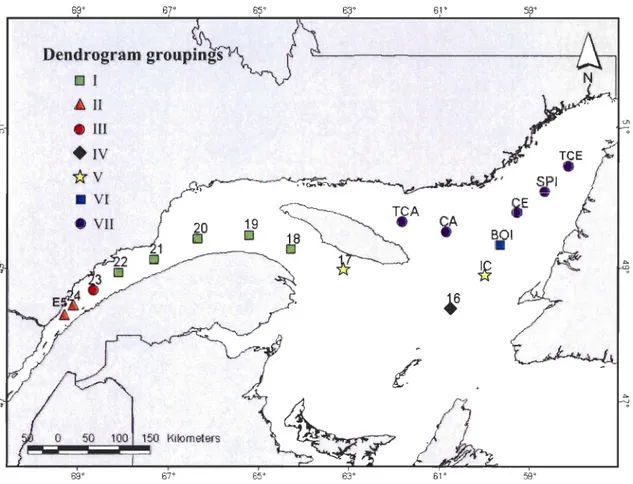
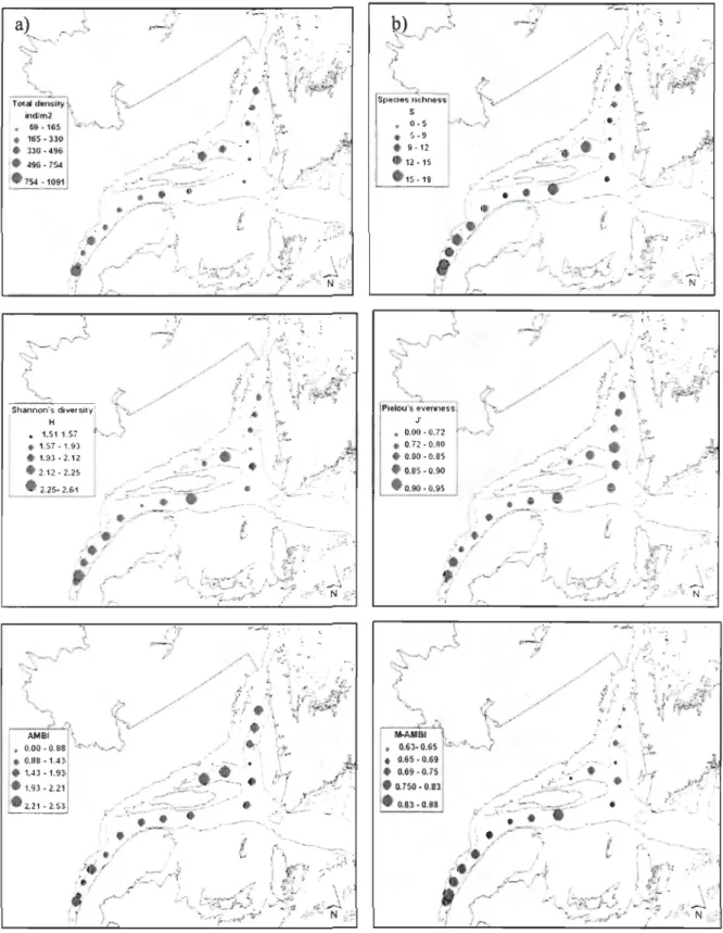
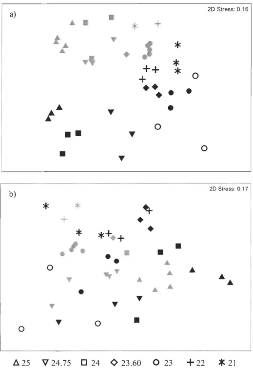
single replicate that were not included in further analyses ... 28 Figure 4. Map of the LSLE and GSL showing the locations of 17 sampling stations and their classification into 7 groups (1 to VII), following clustering analysis of species density data ... 29 Figure 5. Composition (%) of the main macrofaunal functional groups sampled in the deep LSLE and GSL at the different stations in 2005 and 2006. SDF: Surface deposit feeders; SBDF: Subsurface deposit feeders; FF: Filter feeders; C: Carnivores; 0: Omnivores; UC: Unclassified trophic groups ... 33 Figure 6. Total density (ind. mo2), species richness (S), Shannon's diversity (H') and Pielou's evenness (J') at the different sampling stations in the study area ... Erreur! Signet non défini.Figure 7. Two-dimensional nMDS ordination of a) macrofaunal species assemblages and b) functional groups from 1980 (grey), 2005 (black) and 2006 (white) at 7 stations in the LSLE, according to ,; transformed densities (Genus level). Note that only station 23 was sampled in 2006 ... 45 Figure 8. Composition of the main a) taxonomic groups and b) functional groups sampled in the LSLE in 1980 and 2005-06. Others included Chordata, Cnidaria, Nemata (Nematoda), Nemertea, Priapula and Sipuncula. SDF: Surface deposit feeders; SBDF: Subsurface deposit feeders; FF: Filter feeders; C: Carnivores; 0: Omnivores; UC: Unclassified trophic groups ... 46
Figure 9. Mean a) total density (ind. m-2); b) speeies riehness (S); e) Shannon-Wiener's diversity index (H'); d) Pielou's evenness (l'); e) average taxonomie distinetness (~+); and f) variation in taxonomie distinetness (A +) in 1980 and 2005-06 in the
LSLE. Error bars: ± Standard error;
*
above bars indieate signifieant differenees (p < 0.05) ... 50LISTE DES ANNEXES
Annexe 1. Positions et variables environnementales mesurées aux différentes stations d'échantillonnage en 2005 et 2006 ... 87 Annexe 2. Liste des taxons d'invertébrés macrobenthiques récoltés aux différentes stations en 2005 et 2006 ... 88 Annexe 3. Densités moyennes (ind. m,2) des espèces macrobenthiques de chaque groupe fonctionnel pour les stations échantillonnées en 2005 et 2006 ... 91
REMERCIEMENTS
Je tiens tout d'abord à remerCIer particulièrement mon directeur Philippe
Archambault. D'une part, pour sa confiance à mon égard en me proposant ce projet, et
d'autre part, pour avoir partagé avec moi ses nombreuses connaissances et ses bons
conseils. Son amour du métier et son enthousiasme sont contagieux. Un gros merci à ma
co-directrice Karine Lemarchand pour son aide tout au long de ce projet et son
encouragement. Aussi, je désire remercier mon co-directeur feu Gaston Desrosiers, pour
qui j'ai une énorme admiration.
Je voudrais également remerCIer Jesse Gryn et Lisa Treaudecoeli, sans qUI l'identification n'aurait pas été aussi plaisante et qui ont fait un formidable travail. Merci
aussi à tous ceux et celles qui m'ont apporté leur aide lors de l'échantillonnage et le tri des
échantillons: Isabelle Desjardins, Chantale Lachance et Karine Belair. Je ne pourrais passer
sous silence tous les gens qui ont travaillé au laboratoire d'écologie benthique, envers qui
j'ai tissé de véritables liens d'amitié. Je veux spécialement remercier Mélanie Lévesque,
Renald Belley, Annie Séguin, Annick Drouin, Valérie Bélanger et Gwénaëlle Chaillou,
avec qui j'ai pu avoir de belles discussions sur ce projet.
Un gros mercI à l'équipage du Coriolis II pour leur aide lors des mISSIOns
d'échantillonnage sur le terrain. Finalement, j'aimerais remercier le CRSNG pour le
Québec, en tant que récipiendaire de la bourse d'Appui à la Réussite. Merci à ma famille et
INTRODUCTION GÉNÉRALE
Les estuaires sont des environnements transitionnels complexes et dynamiques, caractérisés par des conditions hydrologiques, morphologiques et chimiques très variables (Day et al., 1989). De ce fait, les communautés benthiques vivant dans ces milieux varient à travers différentes échelles spatiales et temporelles, en raison de la grande variabilité des conditions environnementales (Ysebaert et Herman, 2002; Ellis et al., 2006). Les patrons de distribution des organismes benthiques dans de tels milieux sont souvent difficiles à prédire, étant donné la complexité des relations entre les paramètres physiques, les interactions biologiques (compétition et prédation) et le recrutement (Ellis et al., 2006). Un énorme défi pour les écologistes marins est d'identifier et de relier les processus physiques et biologiques responsables de ces patrons, en raison de la grande complexité de l'environnement benthique estuarien (Snelgrove et Butman, 1994). L'étude des habitats benthiques à grande échelle est essentielle dans la gestion des écosystèmes marins, car elle permet d'évaluer les changements environnementaux causés par les perturbations d'origines anthropiques qui surviennent dans les communautés, et plus récemment par les changements climatiques (Freeman et Rogers, 2003).
Rôle de la macrofaune
Le macrobenthos est une composante importante des écosystèmes estuariens et joue un rôle primordial dans la dynamique de ceux-ci. La macrofaune endobenthique forme un
élément essentiel de la chaîne alimentaire estuarienne au nIveau de la productivité secondaire. D'une part, elle est consommée par de nombreux poissons démersaux, oiseaux et crustacés épibenthiques, et d'autre part, elle est une source de nourriture importante pour les populations humaines (Snelgrove, 1998; Herman et al., 1999). De plus, par leurs activités d'alimentation et de bioturbation, les organismes endobenthiques participent activement au transport des particules et ont un impact sur l'oxygénation, le mouvement
vertical et la stabilité du sédiment (Rhoads et Young, 1970; Rhoads, 1974). La macrofaune
contribue également à la récupération des particules de matière organique qui sédimentent
vers le fond marin tels les détritus, les pellettes fécales et les carcasses animales. En se nourrissant de ce matériel, ces organismes, qui servent de proies aux espèces s'alimentant
sur les fonds, assurent le transfert trophique vers la colonne d'eau (Carlson et al., 1997;
Snelgrove, 1998). Le macrobenthos est donc responsable d'une grande part du
fonctionnement des écosystèmes estuariens, et, par conséquent, est très sensible aux
gradients environnementaux estuariens.
Les communautés macrobenthiques sont souvent utilisées comme des indicateurs de
la qualité et de l'état de santé du milieu marin et peuvent donc servir à détecter des
changements de ce milieu. En raison de leurs spécificités écologiques, les organismes macrobenthiques jouent le rôle de bio-indicateurs de modifications de l'environnement et répondent rapidement aux stress de nature anthropique et naturelle (Dauvin, 2007). Leur relative immobilité les empêche d'échapper aux effets d'un stress ou d'une perturbation environnementale, reflétant ainsi les conditions locales. De plus, leur cycle de vie varié,
leur grande diversité et leur tolérance variable à pollution et à la dégradation de l'habitat en font de bons indicateurs (Olsgard et aL, 1997).
Influence des conditions environnementales sur les communautés benthiques
Les communautés benthiques des milieux estuariens sont directement exposées à la
grande variabilité des conditions environnementales caractéristique de ces milieux. En
raison de la variabilité dans la sélection des habitats chez les espèces benthiques, les relations entre la répartition des espèces et les variables environnementales se manifestent par des patrons de distribution (Hall, 1994; Glockzin et Zettler, 2008). De nombreuses
études ont étudié la distribution spatiale des communautés macro benthiques en fonction des
changements des paramètres environnementaux.
L'hétérogénéité spatiale du macrobenthos le long d'un gradient estuarien est
traditionnellement décrite en fonction de la salinité et de la composition du sédiment (Gray,
1981; Holland et aL, 1987; Freeman et Rogers, 2003; Teixera et aL, 2008). De nombreux
travaux ont également décrit les relations entre la distribution et la diversité des espèces et le sédiment dans lequel elles vivent (Sanders, 1968; Rhoads, 1974; Snelgrove et Butman,
1994). Plusieurs études ont démontré l'importance des processus hydrodynamiques et du
substrat (granulométrie et contenu en matière organique) sur la distribution des organismes
benthiques dans un estuaire (Warwick et Uncles, 1980; Warwick et aL, 1991; Rosenberg,
macro benthiques serait fortement reliée à une interaction complexe entre
l 'hydrodynamisme, la dynamique sédimentaire et la biologie benthique (Hall, 1994;
Paterson et Black, 1999; Herman et al., 2001). De plus, Rapoport (1994) et Schaffuer et al.
(2001) suggèrent que l'abondance et la richesse spécifique ont tendance à diminuer en
amont de l'embouchure d'un estuaire. Malgré tout, il est difficile de décrire la distribution
spatiale de la faune benthique en fonction des changements des facteurs environnementaux,
car plusieurs de ces derniers covarient, d'autant plus que les animaux peuvent modifier leur
environnement physique (Ellis et al., 2006).
Parmi toutes les variables environnementales influençant les communautés
endobenthiques, l'oxygène dissous est un facteur limitant pour la macro faune (Diaz et
Rosenberg, 1995; Rabalais et al., 2001; Gray et al., 2002). Dans l'environnement marin,
l'oxygène provenant de l'atmosphère ou du phytoplancton se dissous dans les eaux de
surface et pénètre dans les eaux profondes, permettant ainsi aux organismes benthiques de
respirer. Lorsque l'apport en oxygène dissous en profondeur s'affaiblit ou que le taux de
consommation excède le taux d'approvisionnement, la concentration en oxygène diminue
au point d'atteindre un niveau où l'impact sur la communauté benthique est important
(Diaz, 2001). Cette condition de faible concentration en oxygène, appelée hypoxie, survient
lorsque la concentration en oxygène du milieu est inférieure à 2 ml O2 L-I ou 62,5 ~, soit
le seuil de tolérance de la plupart des organismes benthiques (Gray et al., 2002; Wu, 2002;
Rabalais et al., 2001). Plusieurs scientifiques diffèrent à propos de la définition exacte de
1998). Néanmoins, de nombreux auteurs retiennent la concentration précédente comme hypoxique, car c'est à partir de cette concentration que plusieurs impacts peuvent être observés sur la plupart des espèces marines (Diaz et Rosenberg, 1995; Rabalais et al., 2001).
L'hypoxie dans le Saint-Laurent
L'hypoxie est un phénomène qui peut survenir naturellement dans les milieux où la
circulation d'eau est restreinte, tels les fjords et les zones d'upwelling. Le développement de l'hypoxie en eau profonde est principalement causé par la stratification de la colonne
d'eau, empêchant ainsi les échanges d'oxygène entre les eaux profondes et celles de surface (Cloem, 2001). Cependant, depuis le siècle dernier, l'apport excessif de nutriments dans les
écosystèmes marins côtiers et estuariens, tels les nitrates et phosphates, peut causer des phénomènes d'eutrophisation, contribuant ainsi à l'augmentation de la fréquence et de
l'étendue des zones hypoxiques mondialement (Diaz et Rosenberg, 1995; Gray et al., 2002,
Diaz et Rosenberg, 2008). Cette forte augmentation de la teneur en nutriments, associée à l'augmentation de la population humaine dans les zones côtières, notamment par l'utilisation de fertilisants pour l'agriculture et la déforestation, provoque une augmentation de la productivité primaire pélagique ou benthique. Celle-ci induit une augmentation de l'apport de matière organique de la surface vers le sédiment, la rendant directement disponible aux bactéries et aux organismes détritivores et brouteurs (Heip, 1995). Ce
forte augmentation de la quantité de matière organique vers le sédiment a comme effet d'augmenter le taux de respiration des organismes microbiens benthiques qui reminéralisent la matière organique. Ainsi, les processus de respiration contribuent à la diminution progressive de l'oxygène dissous dans le milieu et peuvent conduire à des conditions hypoxiques (GraU et Chauvaud, 2002; Gray et al., 2002).
Des données historiques provenant de l'estuaire maritime du Saint-Laurent (EMSL) démontrent que les concentrations en oxygène dissous à 300 m de profondeur ont diminué de plus de 50 % durant les 70 dernières années (Gilbert et al., 2005, 2007). En effet, l'oxygène dissous en profondeur a diminué de 125 flmol L-I dans les années 1930 à une
moyenne de 65 flmol L-I pour la période 1984-2003. Des mesures effectuées en 2003, dans
la partie profonde de l'EMSL située dans le Chenal Laurentien, ont révélé une concentration en oxygène dissous inférieure à 60 flmol L·I sur une distance de 110 km, où
la plus faible valeur mesurée était de 51,2 flmol L-I (Gilbert et al., 2005, 2007). Au total,
approximativement 1 300 km2 des fonds de l'estuaire maritime seraient hypoxiques. Un réchauffement des eaux profondes de 1,65 oC de 1930 à 1980 suggère que les changements au niveau des proportions des masses d'eaux entrant dans le Chenal Laurentien jouent probablement un rôle dans la diminution de l'oxygène des eaux profondes. Il est estimé que la moitié à deux tiers de la diminution des concentrations en oxygène peut être expliquée par la diminution de la proportion des eaux froides, douces et oxygénées du courant du Labrador (Gilbert et al., 2005). Une augmentation des flux de carbone organique vers le fond, et conséquemment, de la demande en oxygène du sédiment, expliquerait le tiers
manquant de la diminution de l'oxygène dissous en profondeur (Benoit et al., 2006;
Thibodeau et al., 2006). En effet, une augmentation de la productivité biogénique marine
dans l'estuaire maritime depuis les années 1960 a été observée, indiquée par la signature
isotopique du carbone organique et de l'augmentation du taux d'accumulation des kystes de
dinoflagellés (Thibodeau et al., 2006). De telles variations des indices sédimentaires sont
souvent associées à l'eutrophisation des écosystèmes marins (Cloern, 2001). Toutefois, étant donné le manque actuel de connaissances, il est présentement impossible de prédire l'évolution du budget en oxygène de l'estuaire maritime et du golfe du Saint-Laurent et de
préciser l'impact de la diminution de la concentration en oxygène dissous sur les
communautés endobenthiques.
La déplétion de l'oxygène peut conduire à d'importants changements au niveau de
l'abondance, la distribution, voire même la dynamique des communautés benthiques.
L'hypoxie affecte directement ces communautés benthiques en diminuant le nombre
d'espèces et en augmentant la densité et l'abondance totale de quelques espèces
opportunistes qui survivent (Dauer et al., 1992; Llans6, 1992; Diaz et Rosenberg, 1995;
Gray et al., 2002). La succession de la faune endobenthique et les effets d'une diminution
de la saturation en oxygène à l'interface eau-sédiment ont été décrits par Gray (1992). Ce
modèle montre que la distribution et le comportement de l' épi faune et de l' endofaune
benthique en réponse à un gradient décroissant de saturation en oxygène est semblable au
modèle de Pearson et Rosenberg (1978), décrivant la succession faunique le long d'un
Gray (1992) démontre qu'une déplétion de l'oxygène provoque une diminution du nombre
d'espèces et de la diversité benthique dans le milieu. Ce modèle également aussi que des
conditions de faible oxygénation favorisent quelques petites espèces opportunistes, tirant
avantage d'un changement des conditions environnementales et augmentent en abondance,
au détriment d'espèces plus grosses moins tolérantes. L'appauvrissement en oxygène
conduit également à une réduction de la distribution de la faune en profondeur dans le sédiment, en plus d'une réduction de la diversité fonctionnelle de la communauté.
Figure 1. Schéma de la succession faunique et de la structure du sédiment le long d'un gradient d'enrichissement en matière organique (tiré de Pearson and Rosenberg, 1978).
Macrofaune du Saint-Laurent
Malgré son importance pour les pêcheries commerciales, la macro faune endobenthique profonde dans le Saint-Laurent est encore méconnue, puisque seulement quelques études quantitatives ont été réalisées. Suite aux premiers travaux de Pré fontaine et BruneI (1962) et Peer (1963), les plus récentes études sur la distribution et la diversité endobenthiques dans le Chenal profond de l'estuaire maritime sont celles de Robert (1979) sur les mollusques, Massad (1975) et Massad et BruneI (1979) sur les polychètes et Ouellet (1982) sur la distribution des invertébrés macrobenthiques. Dans le golfe du Saint-Laurent, la structure trophique du macrobenthos a été étudiée à trois stations dans la zone profonde par Desrosiers et al. (2000), alors que Long et Lewis (1987) ont échantillonné quelques stations à ces profondeurs. Cependant, très peu de ces études ont relié les communautés endobenthiques profondes aux conditions environnementales.
Objectifs et hypothèses de l'étude
L'objectif général de la présente étude était de décrire la structure des communautés endobenthiques profondes dans deux régions du Saint-Laurent, soit l'estuaire maritime et le golfe du Saint-Laurent, en termes d'assemblages, de diversité et de groupes fonctionnels. Plus spécifiquement, il s'agissait, d'une part, de décrire la variabilité spatiale des communautés endobenthiques et d'identifier les facteurs environnementaux contrôlant la distribution, la structure et les caractéristiques des communautés endobenthiques
(abondance, diversité, assemblages d'espèces et composition trophique) dans ces deux régions. L'influence des facteurs géomorphologiques (bathymétrie, type de substrat et matière organique) et physico-chimiques (température, salinité et oxygène dissous) sur la structure des communautés a été considérée. Comme la répartition des communautés benthiques est étroitement liée aux conditions environnementales, la structure des communautés devraient être spatialement influencée par les changements au niveau des
variables environnementales. Les conditions hypoxiques observées dans l'estuaire maritime
devrait particulièrement influencer la composition des communautés benthiques présentes dans cette région. D'autre part, les caractéristiques et la structure des communautés endobenthiques, situées dans cette zone hypoxique, ont été comparés à des données historiques afin de déterminer les impacts causés par la diminution d'oxygène. Notre hypothèse est que la diminution temporelle de l'oxygène aura pour effet de modifi er la composition des communautés benthiques et de diminuer l'abondance et la diversité des espèces.
Ce mémoire de maîtrise est présenté sous la forme d'un article scientifique, contenant un chapitre rédigé en anglais. Cet article sera soumis à la revue Estuarine, Coastal and Shelf Science à la suite du dépôt final du mémoire.
CHAPITRE 1
SPATIO-TEMPORAL VARIABILITY OF INFAUNAL COMMUNITY STRUCTURE IN THE DEEP ESTUARY AND GULF OF ST. LAWRENCE (QUEBEC, CANADA) IN RELATION TO ENVIRONMENT AL CONDITIONS
Mylène Bourque and Philippe Archambault
Institut des Sciences de la mer de Rimouski (ISMER), Université du Québec à Rimouski,
31
°
Allée des Ursulines, C. P. 3300, Rimouski, Québec, Canada, 05L 3A11.1 Introduction
Estuaries are complex, dynamic, and highly productive ecosystems characterised by widely
varying hydrological, geomorphological, and chemical conditions (Day et al., 1989). Estuarine benthic communities that inhabit these environments are exposed to a large range of spatial and temporal variations in environmental conditions, resulting in well-developed distribution patterns (Glockzin and Zettler, 2008). Due to the complexity of the estuarine benthic environment, the challenge for marine ecologists is to identify and link the physical and biological processes responsible for these patterns (Snelgrove and Butman, 1994).
Understanding the broad-scale distribution of benthic habitats is essential to the management of marine ecosystems, as it helps to evaluate the natural and anthropogenic influences and effects on these ecological systems.
Many studies have investigated the distribution of soft-sediment macrofaunal communities in relation to environmental conditions. The spatial heterogeneity of macrobenthos along an
estuarine gradient is traditionally described in relation to salinity and sediment composition (Mannino and Montagna, 1997; Ysebaert et al., 2002; Freeman and Rogers, 2003; Teixeira
et al., 2008). Several authors have demonstrated the importance of both hydrodynamic processes and substratum (sediment grain size and organic matter content) in controlling physico-chemical conditions and therefore the benthic organism's distribution within an
estuary (Warwick and Uncles, 1980; Warwick et al., 1991; Rosenberg, 1995). In addition, Rapoport (1994) suggested that total abundance and species richness tended to decrease
with increasing distance from the sea. Thus, macrobenthic faunal patterns will depend on changes in environmental conditions, and small variations in the environment will generate detectable responses in the community (Olsgard et al., 1997). However, spatial distribution patterns of macrobenthic fauna are often hard to predict because the organisms modify their physical environment and many of the physical parameters will co-vary.
A number of univariate and multivariate biodiversity indices are commonly used to follow the changes in benthic communities in their environment and to help scientists and managers to evaluate the status of the ecosystems. However, univariate variables may remain constant even as the species composition changes (Clarke and Warwick, 2001a, Drouin et al., 2009, 2010). Species distribution and community changes should be taken into account, in addition to species richness, when measuring marine biodiversity (Ellingsen, 2001). Multivariate analyses have the potential to be more sensitive to reiatively small changes in faunal composition than univariate methods (Downes et al., 2002; Drouin et al., 2009, 2010). The division of communities into groups or taxa that share similar functional attributes (functional-group) is a common me ans of simplifying the ecological analysis of community structure and function (Bondsdorff and Pearson, 1999). Hence, functional-group responses might be used for the assessment of pollution impacts on marine benthic communities (Clarke, 1993; Bonsdorffand Pearson, 1999). In this way, the AZTI Marine Biotic Index (AMBI) (Borja et al., 2000) and the multivariate approach M-AMBI (Muxica et al., 2007; BoIja et al., 2007) have been used for monitoring purposes, to
analyse the impacts on soft-bottom benthic communities resulting from various human pressures (Borja et al., 2003; Reiss and Kroncke, 2005 ; Labrune et al., 2006).
Oxygen depletion, seasonally common in many stratified marine ecosystems, may have
strong effects on species abundance, distribution, and community dynamics (Dauer et al.,
1992; Diaz and Rosenberg, 1995; Raba1ais et al., 2001). The recent emergence of hypoxic areas in several estuaries seems to be associated with anthropogenic nutrient loading and
coastal eutrophication (Nixon, 1995, Cloem, 2001; Gray et al., 2002; Diaz and Rosenberg,
2008). Severe hypoxia is defined as the threshold below which significant impacts on the
biota can be observed and corresponds to dissolved oxygen concentrations of less than 2 ml O2 L-1 or 62.5 J-lM (Diaz and Rosenberg, 1995; Rabalais et al., 2001). Recent measurements
of dissolved oxygen along the Laurentian Channel of the Lower St. Lawrence Estuary
(LSLE), Canada, revealed the presence of persistent, year-round, hypoxic bottom waters
(Gilbert et al., 2005). Historical data from water samples taken between 300 and 355 m depth in the LSLE revealed that dissolved oxygen concentrations have decreased by more than 50% over the last 70 years, from 125 J-lmol L -1 in the 1930s to about 60 J-lmol L -1 in 2003. In July 2003, an area of approximately 1 300 km2 of the Laurentian Trough was located in the hypoxic zone. One half to two thirds of the decline in oxygen concentration may be explained from a decreasing proportion of cold, fresh, oxygen-rich Labrador Current water entering the Gulf of St. Lawrence (GSL) (Gilbert et al., 2005). The remaining depletion in oxygen is possibly caused by increased fluxes of organic matter to the seafloor, which increase microbial respiration and mineralization (Benoit et al., 2006; Thibodeau et
al., 2006). Faunal succession stages along an hypoxic gradient (Dauer et al., 1992 ; Llanso, 1992; Diaz et Rosenberg, 1995; Gray et al., 2002) suggest that benthic diversity decreases
gradually with decreasing oxygen availability, but it is not clear how benthic cornrnunities
respond to temporal changes in oxygen levels (Katsev et al., 2007).
The deep macrofauna of the LSLE and the GSL is still poorly known. Few quantitative
studies have described the deep benthic infauna cornrnunities in the LSLE. Subsequent to
the earlier investigations of Prefontaine and BruneI (1962) and Peer (1963), the most
qualitative recent study on diversity and distribution of the benthic infauna in the estuary
was realized by Robert (1979) on molluscs and Massad and BruneI (1979) on polychaetes.
More recently, Ouellet (1982) performed a quantitative study of the general distribution of
macrobenthic invertebrates, while the trophic structure of macrobenthos in the GSL was
sampled and analysed by Desrosiers et al. (2000) and Long and Lewis (1987). However,
none of these studies linked the environmental conditions to deep benthic infauna
communities.
The main objective of the present study was to describe the macrobenthic infaunal
cornrnunities from two distinct regions of the St. Lawrence, the Lower Estuary (LSLE) and the Gulf (GSL). Specifically, we exarnined spatial patterns of benthic cornrnunity
characteristics (e.g. abundance, diversity, functional groups) and the structure of benthic
assemblages. The spatial distribution of macrofauna was evaluated with the environmental
in order to detennine the role of such factors in structuring community structure. As the distribution of communities is linked to environrnental conditions, we hypothesize that benthic communities should be strongly influenced by spatial changes in oxygen concentration. In particular, benthic assemblages located in the hypoxic zone should be different compared with those from locations not experiencing hypoxic conditions. We a1so quantified temporal variations among years in macrobenthic community structure in the hypoxic area of the LSLE using available historical data. Based on the outcomes of previous studies, we hypothesize that the temporal decrease in oxygen concentration should cause a shift in species composition, with an increase in opportunistic and tolerant species, and a decrease in diversity indices. Finally, we also want to establish the Ecological Quality Status of the deep channel of the Lower St. Lawrence Estuary and Gulf.
1.2 Material and methods
1.2.1 Study area
The Gulf of St. Lawrence (GSL) is a highly-stratified, semi-enclosed sea, connected to the North Atlantic Ocean through the Cabot Strait and the Strait of Belle-Isle. A major topographic feature of the system is the Laurentian Channel (LC), a deep submarine valley (250 - 500 m) that furrows the Gulf, extending from the margin of the North Atlantic Ocean to the Lower St. Lawrence Estuary (LSLE) (Fig. 2). The LC ends at Tadoussac where the bathymetry rises abruptly from 350 to 25 m over a distance of 16 km (Koutitonsky and
Bugden, 1991). Two other deep channels branch off from the LC between Newfoundland and Anticosti Island: the Esquiman Channel and the Anticosti Channel (Fig. 2). The circulation in the Laurentian Channel is estuarine, with water flowing seaward in the surface layer and landward in the deep layer (Saucier et al., 2003). The water colurnn of the LC is stratified and can be divided vertically into three characteristic layers: 1) a low salinity (- 25) surface layer, 2) an intermediate cold layer extending from 50 to 150 m depth, with saline water (32 to 34), and 3) a deep, warmer and saltier (> 34) layer, that is a
mixture of Labrador CUITent and North Atlantic waters (Dickie and Trites, 1983). A permanent pycnoc1ine is located between 100 and 150 m that isolates deep waters from the atmosphere (Petrie et al., 1996). Under these conditions, oxygen concentration decreases gradually in the bottom waters, possibly because of changes in water temperature,
respiration, and organic matter mineralization (Gilbert et al., 2005). Consequently, more oxygen is lost by vertical diffusion than can be replenished from the oxygen-rich surface waters, causing ever-decreasing oxygen levels from the mouth of the LC to the head of channels, where bottom waters are oider (Coote and Yeats, 1979).
1.2.2 Field sampling methods and laboratory analyses
Sampling was conducted during two cruises, in summer 2005 (August 20-26) and 2006 (August 14-22), on-board the RN Coriolis II. A total of 17 stations, extending 522 to 1049 km from the Laurentian Channel mouth, sampled deep waters of the LSLE and GSL,
deeper part of the LSLE and at the northwestem end of Anticosti Island, along the longitudinal axis of the Le. Nine stations were sampled in 2006 in the GSL, along the Laurentian, Anticosti and Esquiman Channels. Station 23 (Fig. 2), which is located in the hypoxic zone of the LSLE offshore of Rimouski, was sampled during two consecutive
years (2005 and 2006).
At each station, macrobenthic infauna samples in three replicates were collected
with a van Veen grab (0.l25 m2) and sieved on-board through a 1 mm mesh, to enable quantitative comparisons with the historical faunal data from Ouellet (1982). The retained material was preserved in a buffered 5% formaldehyde-saline solution and macrofauna was stored in 70% ethanol after sorting. Macrobenthic organisms were counted and identified to the lowest taxonomic level possible. Macrofaunal species were c1assified into six functional groups by feeding type (surface deposit feeders, subsurface deposit feeders, filter feeders,
carnivores, omnivores, and unc1assified trophic group), according to the classification and observations of Fauchald and Jumars (1979), Desrosiers et al. (1986, 2000) and Gage and Tyler (1992). For each sample, total macrofaunal density (individual m-2) was calculated for each functional group and species.
Surface sediment sub-samples were also collected from a box core, for later sediment property determination. Sediment composition was analyzed using a laser diffraction grain size analyzer (Beckman Coulter Counter LS 13 320), allowing the differentiation of parti cl es ranging from 0.4 ~m to 2000 ~m in size, according to Blott et al.
(2004). Prior to its introduction into the instrument, the sub-sample of 1 g of sediment was
disaggregated in 10 ml of a 1 g
ri
sodium hexametaphosphate solution (Calgon) and 40 mlof distilled water and shaked for 3h. An ultrasonic treatment was applied before and during
the sample run in the instrument to improve the disaggregation of the sample (Blott et al.,
2004). The frequency distribution of grain size diameter was analyzed using the GRADISTAT pro gram (Blott and Pye, 2001). Grain size frequency per sample was expressed as percentage of sand, silt, and clay, and mean grain size (~m) was calculated. Total organic matter content (TOM) was measured as 10ss upon ignition at 500 oC for 12 h on 1 g of surface sediment and expressed as a percentage of total sample mass (Dean,
1974).
Physico-chemical data, su ch as depth, temperature, salinity and dissolved oxygen,
were measured at each station with a Seabird® model SBE 19 CTD instrument. The
dissolved oxygen concentration was determined by the Winkler method (Carrit and
Carpenter, 1966), for individual bottom water samples collected with Niskin bottles mounted on a rosette sampler at 5 m above the seafloor.
1.2.3 Temporal historical data
A literature review of historical data regarding the the deep-water macrobenthos of the LSLE and GSL (i.e. > 250 m) revealed only a few studies that contained quantitative data The macrobenthic faunal data from Ouellet (1982) were used to conduct temporal
eomparisons with 2005 and 2006 datasets. From these data, seven stations with the same position as those in the present study were seleeted for temporal analyses (Fig. 2b). These stations were sampled in 1980 along the longitudinal axis of the
Le
with a 0.125 m -2 van Veen grab (Ouellet, 1982). Eaeh sampling station was represented by three pooled grabs, except at stations 23, 24 and 25, where five triplieated pooled grabs were sampled. AIl maerobenthie abundanee data were transformed in density or numbers m·2 (ind. m-2). For historieal data, taxonomie names were verified and updated using the Integrated Taxonomie Information System on-line database (www.itis.gov).02550 h) o 1020 '"' a) QUEBEC
ilomet~RUNSWICK
\ Tadoussac 40 60 80 Kilom rFigure 2. a) Study area showing the location of the 17 sampling stations in 2005 (.) and 2006 (D), with infauna and environmental data. Station 23 was sampled in both 2005 and 2006 (0). b) Map of the St. Lawrence estuary showing the location of the seven stations
with infauna historical data, sampled in 1980 and 2005 ( . ), except for station 23 which was also sampled in 2006 (e ).
1.2.4 Statistical analyses
Spatial and temporal variability in macrobenthic community structure was analyzed with univariate and multivariate procedures. Methods of Clarke and Warwick (1994,
2001a) using the PRlMER software v. 6.0 (Clarke and Gorley, 2001), were used to detect spatial and temporal patterns in community structure. AlI multivariate analyses were based on the Bray-Curtis similarity (Bray and Curtis, 1957) ca1culated on square-raot
(-1)
transformed data. This transformation served to reduce the influence of very abundant species, so that the less-dominant, and even the rare species, would play sorne role in determining similarity between samples (Clarke, 1993; Clarke and Warwick, 1994). Before computing the similarity matrix, taxa that appeared once or in only one sample were removed from the datas et, as suggested by Clarke and Warwick (1994).Spatial variability
Sampling stations with similar macrobenthic assemblages were regrouped using a hierarchical classification method (CLUSTER analysis) employing group-average linking.
Taxa or species that were predominantly responsible for the similarity within clusters were identified by the similarity percentage procedure (SIMPER). This analysis ranked each species' percentage contribution, based on
-1
transformed densities, to the similarity within the cluster (Clarke and Warwick, 200Ia).Univariate indices of infaunal community diversity (total density (ind. m-2), species
richness (S), Shannon-Wiener diversity index (H', loge) and Pielou's evenness index (1':
H '/log S» were calculated for aU replicated samples. Species were assigned to one of the
five ecological groups used by BOlja et al. (2000) based on their sensitivity to organic
enrichment, from very sensitive species (group 1) to first-order opportunistic (group V).
The organisms thus categorized were used to calculate a global index of community
disturbance (AMBI - see Borja et al., 2000) using the software AMBI v 4.0
(http://\Vww.azti.es). The M-AMBI index was also calculated, combining AMBI, richness,
and Shannon diversity, to give a multivariate index (Muxika et al., 2007). In addition,
average taxonomic distinctness (L1l and variation in taxonomic distinctness (A +) were
calculated on macrofaunal densities (DIVERSE analysis, PRIMER). These indices are
pertinent measures of biodiversity and provide important tools to compare meta-analyses over large spatial and temporal scales (Clarke and Warwick, 2001b).
The relationships between environmental variables and macrobenthic community
structure were examined with a BIO-ENV analysis (Clarke and Warwick, 1994). This procedure was used to find the combination of abiotic factors which best accounted for
species and functional groups community structure. Because of the dissimilarity in
environmental conditions between the LSLE and the GSL, these two regions were analyzed separately. Multiple regression analyses were used to examine the relationships between
univariate indices (total density, S, H', J', L1 +, and A +) and environmental parameters
content). Two criteria, the adjusted r2 and the Akaike Information Criterion (AIC), were used to select those environmental variables to be included in the model that best explained the univariate diversity indices. Collinearity was examined using a matrix of correlation
coefficients between the different environmental variables, as recommended by Quinn and
Keough (2002). For aU univariate analysis, the assumptions of homogeneity of variances and normality were confirmed using the graphical exarnination of residuals (Quinn and Keough, 2002) and the Shapiro-Wilk's test, respectively. To respect the statistical
assumptions, a logarithmic transformation was applied to the univariate indices when necessary and is indicated in the tables and figures.
Temporal variability
Temporal variability in the structure of macrobenthic infauna assemblages structure
was identified using a pem1utational multivariate analysis of variance (PERMANOVA) with two sources of variation (Anderson, 2001; McArdle and Anderson, 2001) performed with 9999 random permutations of the appropriate units. Sources of variation were 1) year
(fixed with 3 levels: 1980, 2005, and 2006), 2) station (fixed with 7 levels: E5, 24.75, 24,
23.60,23,
n
,
21), and 3) the interaction among these factors (3 years by 7 stations). When there were too few possible pem1utations to obtain a reasonable test, a p-value was calculated using 9999 Monte Carlo drawn from the appropriate aSy1nptotic permutationdistribution (Terlizzi et al., 2005). Significant tenns in the full model were examined
Multivariate patterns in macrobenthic assemblages were visualized using non-metric multidimensional scaling (l\1DS) ordination of dissimilarity matrices on -V transformed data.
Discriminating species between years were recognized using the SIMPER procedure, based on -V transformed data. In order to detect temporal patterns in benthic infauna community characteristics in the LSLE, two-way analyses of variance (ANOY A) between stations and
sampling years were used to compare univariate community characteristics (total density,
S, H', J', ô+ and i\+), using the Tukey's test to calculate a posteriori comparisons
(Underwood, 1997). The assumptions of homogeneity of variances and normality were
verified using the graphical examination of residuals (Quinn and Keough, 2002) and the Shapiro-Wilk' s test, respectively.
1.3 Results
1.3.1 Spatial structure ofmacrobenthic infaunal communities
A total of 80 species or taxa were identified in 2005 and 2006, within 52 different families, 23 orders, 14 classes and 9 phyla. Mean densities of macrobenthic organisms
varied considerably in the study area, ranging from 69.3 to 754.7 ind. m-2 in the GSL, and 154.7 to 1091 ind. m-2 in the LSLE. Polychaeta were the dominant taxa in terms of density in the entire study area, varying from 55 % (station 17) to 94 % (station SPI) of the total macrofauna1 composition. Polychaetes were more important in the LSLE than in the GSL,
where they accounted for 82 % and 78 % of the total composition, respectively. Among the dominant species, the spionid Spiophanes kroyeri and the ampharetid Ampharete
lindstroemi were more abundant in the LSLE, whereas the nereid Ceratocephale love ni and the lumbrinerid Lumbrineris sp. dorninated in the GSL. Taxa such as Echinodermata, Arthropoda, and Mollusca were found in lower abundance in the study area, representing 6.3%, 5.3%, and 4.6% of the total composition, respectively. Regionally, the composition of molluscs was higher in the LSLE, due to the presence of the bivalve Nucula delphinodonta, while arthropod and echinoderm compositions were higher in the GSL, due mainly to important densities of the gammarid Harpinia propinqua and the ophiurid
Amphiura sundevalli. Other taxa, from phyla Nematoda, Cnidaria, Nemertina, Sipuncula,
and Chordata were also observed in both regions, representing 2.3% of the benthic
composition in the LSLE and 4.9% in the GSL.
The CLUSTER analysis segregated the macrofauna from the study area into seven main groups (clusters) of stations: five groups at a 33% similarity level (1 to V) and two
groups at a 42% similarity level (VI and VII) (Fig. 3). Two clusters were located in the LSLE (II and III) and four in the GSL (l, IV, V, and VI), as shown in Figure 4. Cluster VI
was located at the intersection between both regions. The five taxa predominantly
responsible for the sirnilarity within clusters are presented in Table 1 a. Cluster II stations
(ES and 24) were found at the head of the LSLE and are characterized by high abundances of A. lindstroemi, S. kroyeri and Trochochaeta multisetosa (Table 2, Fig. 4). Most of the replicates of station 23, which is located across the shore from Rimouski and sampled in
2005 and 2006, belong to Cluster III (Table 2, Fig. 4). Polychaetes in high abundance, such as A. lindstroemi, C. loveni, and Myriochele heeri, contributed largely to the sirnilarity within this group. Clusters VI and VII inc1uded most of the sampling stations and consisted predorninantly of stations located in the GSL (Fig. 3). Cluster VI stations were found at the upper end of the LSLE (22 and 21) and at the northeastern end of Anticosti Island (20, 19 and 18), and were characterized by C. loveni, Amphiura sundevalli, and Lumbrineris sp. (Table 2, Fig. 4). Conversely, Cluster VII stations (TCA, CA, TCE, CE and SPI) were located in the Anticosti and Esquiman Channel s, in the northeastern part of the GSL (Table
2, Fig. 4). According to the SIMPER analysis, species contributing principally to the differentiation from other clusters were Lumbrineris sp., C. loveni, and Heteromastus
filiformis (Table la). Species such as Tharyx sp., Lumbrineris sp., and Antalis occidentale
largely dorninated Cluster V, which was composed of stations 17 and IC, located at the mouth of the Laurentian Channel and the Anticosti and Esquiman channels, respectively
(Table 2, Fig. 4). Station BOl (Cluster 1) was separated from the others by the presence of
Onuphis opalina, Axinopsida sp., Lumbrineris sp., and Pennatula aculeata (Table 2, Fig.
4). Cluster IV (station 16), located in the GSL west of Cabot Strait, was characterized by
o
20 , -~ Q '-" .èï
:
40 ~-.
-S 'r;; .~
-
:... 60 ::::1 U 1 >. ~ :... CQ 80 100 l 1~
I
-
-
n
~
n
n
i
J
--.
-
----
= = =
=
= = = = =
:1J2:-- :1J2:--:1J2:--=:L
-33 % 42 % ,-L-, r-
1Rn~,---'----~~NM~NM~NM~NNMMNNM~MN~~M~NMM~NM~MN~M~N~NMNM~N~NMNM~N~M 1 1 1 1 1 1 1 1 1 1 1 1 1 1 1 1 1 1 1 1 1 1 1 1 1 1 1 1 1 1 1 1 1 1 1 1 1 1 1 1 1 1 1 1 1 1 1 1 1 1 1 1 1 1 NI6 6 6 Lfl Lfl Lfl ~ ~ ~ ~I ~I NI ~I NI ~ ~ ~ ~ ~ ~ ~ ~ ~ N N N gj gj gj ~ C3 C3 C3 CL C3 C3 C3 ~ ~ ~ CL CL ~ ~ ~ ~ ~ S2 ~ ~ ~ S2 S2 ~rororo ~~~~~ ~rrrrrr ~~ *~ oC >- < >-1•
A Il III•
< >-VI D Samples < >-~ * oC >-VII•
IV•
*
VFigure 3. a) Hierarchical c1ustering with group average linking of-V transformed densities for each replicate, using Bray-Curtis
similarity (%). The grouping of stations corresponded to the horizontal lines at 33 % similarity level (1 to V) and 42 %
69' 67' Dendrogram groupings D 1 ~ 11 e lll +IV
1rv
• VI • VII 20 D o 50 100 150 Kilometers 69' 67' 65' 19 D 65' 63' 61' 59'Figure 4. Map of the Lower St. Lawrence Estuary (LSLE) and Gulf of St. Lawrence (GSL)
showing the locations of 17 sampling stations and their classification into 7 groups (I to
Table 1. Results of SIMPER analyses showing taxa with the greatest contribution (%) to the average Bray-Curtis similarity, based on ,j transformed densities, of compared replicates within each cluster (1 to VII) as weIl as the average sirnilarity (%) for each group ofsamples.
Species Contr. (%) Species Contr. (%)
Cluster 1 (Avg. sirnilarity = 49.38)
Onuphis opalina 37.46
Axinopsida sp. 31.44
Lumbrineris sp. 11.61
Pennatula aculeata Il.27
Cluster III (Avg. similarity
=
42.09)Ampharete lindstroemi 31.12 Ceratocephale loveni Myriochele heeri Axinopsida sp. Tharyx sp. 18.84 15.08 6.92 4.63 Cluster V (Avg. sirnilarity
=
44.24)Tharyx sp. 21.18
Lumbrineris sp. 16.37
Antalis occidentale 12.85
Harpinia propinqua
Amphiura sundevalli 8.23 7.95
Cluster VII (Avg. similarity = 53.92)
Lumbrineris sp. 24.74
Ceratocephale loveni 19.54
Heteromastus filiformis 19.12
Tharyx sp. 9.99
Ampharete lindstroemi 4.19
Cluster II (Avg. sirnilarity
=
46.51)Ampharete lindstroemi 17.40
Spiophanes kroyeri 16.07
Trochochaeta multisetosa Il.80
Terebellides stroemi 10.20
Maldanidae 9.57
Cluster IV (Avg. sirnilarity
=
44.05)Lumbrineris sp. 30.36
Amphiura sp. 24.85
Tharyx sp. 21.89
Harpinia propinqua
Nemertea 7.88 7.88
Cluster VI (Avg. sirnilarity
=
53.71) Ceratocephale loveni 25.83Amphiura sundevalli 17.34
Lumbrineris sp. 14.91
Heteromastus filiformis 10.77
The changes in macrofaunal functional group distribution along a transect in the
LSLE and the GSL are illustrated in Figure 5. The trophic structure of the LSLE was
dominated by surface deposit feeders (SDF), contributing to 40-76% of total macrofaunal
composition at stations E5 to 21. Surface deposit feeders, such as S. kroyeri, A. lindstroemi,
and T. multisetosa, dominated at the head of the LSLE (stations E5 and 24), where
subsurface deposit feeders (SBDF) like Maldanidae were also abundant. Continuing in this
direction, species such as A. lindstroemi, S. kroyeri, and M. heeri were the most abundant
SDF at upstream stations (stations 24 and 23). For example, near the boundary between the
LSLE and the GSL (stations 22 and 21), SDF M. heeri and A. lindstroemi were once again dominant, but decreased gradually. A consequent increase in omnivores (0) was observed
along the Laurentian Channel, mainly due to the increasing importance of C. loveni, A.
sundevalli, and Lumbrineris sp. (stations 20, 19, and 18). Thereafter, a small decrease in
omnivorous species was noted at the intersection of the Laurentian, Anticosti and Esquiman
channels (stations 17, 16 and IC), whereas SDF species increased. Moreover, a high
number of SBDF, su ch as Maldanidae, was observed at the intersection of Anticosti and
Esquiman channe1s (station IC), and were more important in the GSL than in the LSLE.
These organisms were also abundant at the head of Anticosti and Esquiman channels
(stations TCA and TCE), counting for 38% and 27% of the total macrobenthic composition,
respectively, ev en as omnivorous species like Lumbrineris sp. were dominant in this region
of the GSL. A great number of SDF such as Tharyx sp., along with omnivores (i.e.,
Lumbrineris sp. and H. filiformis), were observed in the Anticosti Channel (station CA). However, only omnivores dominated stations in the Esquiman Channel (stations CE and
SPI), with high abundances of C. loveni and Lumbrineris sp. Omnivorous species, such as O. Opalina and Lumbrineris sp., also dominated the trophic structure at station BOL
Among the other functional groups, Carnivores (C) and Filter feeders (FF) had only a minor presence in the study areas. A small increase in carnivore composition was observed in the LSLE, varying from 1 to 9.6 % from the head to the boundary of the GSL, whereas the highest abundance ofFF was seen at station 23. In the gulf, both C and FF dominated at station BOl, representing respectively up to 11.5 and 15.3 % of the total benthic community. Sea pens (Pennatulacea, P. aculeata), were the most important carnivorous species, whereas bivalve species of Astartidae (Astarte undata) and Thyasiridae (Axinopsida sp.) were the most important filter feeders.
Il III VI IV V 1 VII
tE :> oe: :>
100% oe: :>
~ oe: :>~tE :. Cluster groups
90% 80% 70% ,-.. DUC '::!( 60%
'"
' - ' - 0 c:.::
.... 50% - C 'c;; 0 c. - FF E 0 40% U DSBDF 30% 1_- - - - -
1-
1- - -
-
-
1 1 - SDF 20% 10% 0% V) '1" N N 0 0\ 00 'D r- U0
«
«
U.l 0:: U.l U.l N 1 1 N N N -U U U U cr, cr, co VJ f--< N N f--< StationsFigure 5. Composition (%) of the main macrofaunal functional groups sampled in the deep LSLE and GSL at the different
stations in 2005 and 2006. SDF: Surface deposit feeders; SBDF: Subsurface deposit feeders; FF: Filter feeders; C: Carnivores;
Univariate indices revealed differences among stations (Fig. 6). Total mean density of macrofauna species was highest at the head of the LSLE (ES), whereas station BOl
exhibited the lowest value. This index was also high at station 22 and at the head of the Anticosti and Esquiman channels (TC A and TCE), while stations 16 and lC showed low densities of organisms. A similar spatial pattern was seen for AMBI and species richness
(S), with the highest and lowest values observed at stations ES and BOl, respectively. High
values of Shannon-Wiener diversity (H ') were observed at stations 17 and CA, whereas
lower diversities were found at stations BOl and 19. Conversely, station BOl exhibited the
highest evenness (J'), followed by stations 17 and 16, while low values of J' were observed at stations ES, TCA and 22. Values ofM-AMBI that are smaller than 0.62 are indicative of community moderate1y disturb to very disturb «0.20). However none on the values
calculated in the LSLE and in the GSL exhibited values smaller than 0.62 and many values
were above 0.83, which means that the Ecological status are high (Fig. 6). This was the
~Shllnnon'5 diversilY1 H • 1.511.57 • 1.57·1.93 . 1.93·2.12 • 2.12 • 2.25 , i . 2.25-2.61 [ "---,.~,---_. : 1)" $-"~: "
:
.
,
j
'/
M-AMBI :. 0.63- 0.65..
' ('r i. 0.65·0.69 i. 0.69·0.75l
.
0.750 -0.831
.
0.83.0.88 .' , ~" .";::/~ N 2~ ./~. ~~,.
(Figure 6. Total density (ind. m·2), species richness (S), Shannon-Wienner diversity (H'),
1.3.2 Relationships between macrobenthic community structure and environmental factors Stations sampled in 2005 and 2006 in the LSLE and GSL were distributed across a
wide range of environmental conditions: depth (median: 323 m; range 257-434 m), bottom
temperature (median: 5.40 oC; 4.87-5.79 oC), bottom salinity (median: 34.61 PSU; 34.38
-34.86 PSU), oxygen saturation (median: 34.58%; 21.21-58.13%), mean grain size (median:
10.70 !lm; 7.81-20.38 !lm), and total organic matter content (median: 3.60%; 2.45 to
5.78%) (Table 1). Silt was the dominant grain size fraction in the LSLE and GSL, ranging
from 65.6% to 88.5%. The clay fraction represented 10% to 32.6% of the sediment
composition in the study area.
ln the LSLE, mean grain size, salinity, and temperature best explained the pattern of
species assemblages (rs = 0.432) (Table 3a), with mean grain size as the single variable
with the highest correlation Crs
=
0.412). ln the GSL, temperature and salinity provided thebest explanation of species composition (rs
=
0.460). The distribution pattern of functionalgroups in the LSLE was best correlated with temperature as a single variable (rs
= 0
.455)and the combination of mean grain size, total organic matter, salinity, and temperature (rs
=
0.465). The highest correlation between functional assemblages and environmental
parameters in the GSL was observed for temperature (rs
=
0.282), although the relation wasrelatively weak (Table 3b), due to several inter-correlations between environmental
parameters. High correlations in the LSLE were observed for salinity and oxygen saturation
(0.794). In the GSL, mean grain size was highly correlated with organic matter content (0.837), whereas temperature was strongly negatively-correlated with depth (-0.809). These correlations could have a strong impact on analyses, as the effect of other important
variables would not be detected. However, physical variables characteristic of estuaries,
such as substrate type, salinity and temperature, are often strongly linked (Clarke and Green, 1988). As proposed by Callaway et al. (2002), it was decided to include aIl
environmental variables in the analysis because the inter-correlations between environmental factors were not consistent for the entire study area.
In the LSLE, multiple linear regressions models explained up to 75% and 62% of
total density and species richness (S) variances respectively, 20% of diversity (H') variance and 57% of evenness (J') variance (Table 4a). In addition, 31 % of average taxonomic distinctness (f1l variance and 26% of taxonomic distinctness (A +) variance were explained in this analysis, whereas the models explained 65% and 90% of AMBI and M-AMBI variances, respectively. This analysis showed that depth and mean grain size best explained total density, S, H ', J', AMBI, and M-AMBI. Also, oxygen saturation best explained total density, S, J'and A+, whereas f1+, A+, AMBI, and M-AMBI were best explained by total organic matter. Regression models calculated for the GSL explained up to 64% of total density, 23% of S, 15% of H " and 35% of J' (Table 4b). Up to 47% and 17% of f1 + and A +
variances, respectively, was explained by the models, whereas they explained up to 58% and 59% of AMBI and M-AMBI variances. Temperature was present in aIl regression models, except for J', whereas mean grain size seemed to explain, in part, total density, S,
H', and ,:1+. Oxygen saturation best explained total density, H', and J', while ,:1+ and A+