HAL Id: hal-01061578
https://hal.archives-ouvertes.fr/hal-01061578
Submitted on 11 Sep 2014
HAL is a multi-disciplinary open access
archive for the deposit and dissemination of
sci-entific research documents, whether they are
pub-lished or not. The documents may come from
teaching and research institutions in France or
abroad, or from public or private research centers.
L’archive ouverte pluridisciplinaire HAL, est
destinée au dépôt et à la diffusion de documents
scientifiques de niveau recherche, publiés ou non,
émanant des établissements d’enseignement et de
recherche français ou étrangers, des laboratoires
publics ou privés.
convolutive mixtures of non-stationary signals in the
time-frequency domain
Roland Badeau, Mark Plumbley
To cite this version:
Roland Badeau, Mark Plumbley. Multichannel high resolution NMF for modelling convolutive
mix-tures of non-stationary signals in the time-frequency domain. IEEE Transactions on Audio, Speech and
Language Processing, Institute of Electrical and Electronics Engineers, 2014, 22 (11), pp.1670-1680.
�hal-01061578�
Multichannel high resolution NMF for modelling
convolutive mixtures of non-stationary signals
in the time-frequency domain
Roland Badeau, Senior Member, IEEE, Mark D. Plumbley, Senior Member, IEEE
Abstract—Several probabilistic models involving latent com-ponents have been proposed for modelling time-frequency (TF) representations of audio signals such as spectrograms, notably in the nonnegative matrix factorization (NMF) literature. Among them, the recent high resolution NMF (HR-NMF) model is able to take both phases and local correlations in each frequency band into account, and its potential has been illustrated in applications such as source separation and audio inpainting. In this paper, HR-NMF is extended to multichannel signals and to convolutive mixtures. The new model can represent a variety of stationary and non-stationary signals, including autoregressive moving aver-age (ARMA) processes and mixtures of damped sinusoids. A fast variational expectation-maximization (EM) algorithm is proposed to estimate the enhanced model. This algorithm is applied to piano signals, and proves capable of accurately modelling reverberation, restoring missing observations, and separating pure tones with close frequencies.
Index Terms—Non-stationary signal modelling,
Time-frequency analysis, Nonnegative matrix factorisation,
Multichannel signal analysis, Variational EM algorithm.
I. INTRODUCTION
N
ONNEGATIVE matrix factorisation was originally intro-duced as a rank-reduction technique, which approximates a non-negative matrix V ∈ RF ×T as a product V ≈ W Hof two non-negative matrices W ∈ RF ×S and H ∈ RS×T
with S < min(F, T ) [1]. In audio signal processing, it is often used for decomposing a magnitude or power TF representation, such as a Fourier or a constant-Q transform (CQT) spectrogram. The columns of W are then interpreted as a dictionary of spectral templates, whose temporal activations are represented in the rows of H. Several applications to audio have been addressed, such as multi-pitch estimation [2]– [4], automatic music transcription [5], [6], musical instrument recognition [7], and source separation [7]–[10].
In the literature, several probabilistic models involving la-tent components have been proposed to provide a probabilistic framework to NMF. Such models include NMF with additive Gaussian noise [11], probabilistic latent component analysis (PLCA) [12], NMF as a sum of Poisson components [13], and NMF as a sum of Gaussian components [14]. Although they have already proven successful in a number of audio ap-plications such as source separation [11]–[13] and multipitch
Roland Badeau is with Institut Mines-Telecom, Telecom ParisTech, CNRS LTCI, 37-39 rue Dareau, 75014 Paris, France.
Mark D. Plumbley is with the Centre for Digital Music, Queen Mary University of London, Mile End Road, E14NS London, UK.
estimation [14], most of these models still lack of consistency in some respects.
Firstly, they focus on modelling a magnitude or power TF representation, and simply ignore the phase information. In an application of source separation, the source estimates are then obtained by means of Wiener-like filtering [8]–[10], which consists in applying a mask to the magnitude TF representation of the mixture, while keeping the phase field unchanged. It can be easily shown that this approach cannot properly separate sinusoidal signals lying in the same frequency band, which means that the frequency resolution is limited by that of the TF transform. In other respects, the separated TF representation is generally not consistent, which means that it does not correspond to the TF transform of a temporal signal, resulting in artefacts such as musical noise. Therefore enhanced algorithms are needed to reconstruct a consistent TF representation [15]. In the same way, in an application of model-based audio synthesis, where there is no available phase field to assign to the sources, reconstructing consistent phases requires employing ad-hoc methods [16], [17].
Secondly, these models generally focus on the spectral and temporal dynamics, and assume that all time-frequency bins are independent. This assumption is clearly not relevant in the case of sinusoidal or impulse signals for instance, and it is not consistent with the existence of spectral or temporal dynamics. Indeed, in the case of wide sense stationary (WSS) processes, spectral dynamics (described by the power spectral density) is closely related to temporal correlation (described by the autocovariance function). Reciprocally, in the case of uncor-related processes (all samples are uncoruncor-related with different variances), temporal dynamics induces spectral correlation. In other respects, further dependencies in the TF domain may be induced by the TF transform, due to spectral and temporal overlap between TF bins.
In order to overcome the assumption of independent TF bins, Markov models have been introduced for taking the local dependencies between contiguous TF bins of a magnitude or power TF representation into account [18]–[20]. However, these models still ignore the phase information. Conversely, the complex NMF model [21], [22], which was explicitly designed to represent phases alongside magnitudes in a TF representation, is based on a deterministic framework that does not represent statistical correlations. More recently, two probabilistic models have been proposed, which partially take the phase information into account. The multichannel NMF presented in [23] is able to exploit phase relationships between
different sensors via the mixing matrix, but the phases and correlations of source signals over time and frequency are not modelled. The infinite positive semidefinite tensor fac-torization method presented in [24] is able to exploit phase information by modelling correlations over frequency bands, but correlations over time frames are still ignored.
Alternatively, the high resolution (HR) NMF model that we introduced in [25], [26], is able to model both phases and correlations over time frames (within frequency bands) in a principled way. We showed that this model offers an improved frequency resolution, able to separate sinusoids within the same frequency band, and an improved synthesis capability, able to restore missing TF observations. It can be used with both complex-valued and real-valued TF representations, such as the short-time Fourier transform (STFT) and the modified discrete cosine transform (MDCT). It also generalizes some popular models, such as the Itakura-Saito NMF model (IS-NMF) [14], autoregressive (AR) processes [27], and the ex-ponential sinusoidal model (ESM), commonly used in HR spectral analysis of time series [27].
In this paper, HR-NMF is extended to multichannel signals and to convolutive mixtures. Contrary to the multichannel NMF [23] where convolution was approximated, convolution is here accurately implemented in the TF domain by following the exact approach proposed in [28]. Consequently, correla-tions over time frames and over frequency bands are both taken into account. In order to estimate this multichannel HR-NMF model, we propose a fast variational EM algorithm. This paper further develops a previous work presented in [29], by providing a theoretical ground for the TF implementation of convolution.
The paper is structured as follows. The HR-NMF model is first introduced in the time domain, then the filter bank used to compute the TF representation is presented in Section II. We show in Section III how convolutions in the original time domain can be accurately implemented in the TF domain. The multichannel HR-NMF model in the TF domain is presented in Section IV, and the variational EM algorithm is derived in Section V. This model is applied to audio inpainting and source separation in Section VI. Finally, conclusions are drawn in Section VII.
NOTATION
The following notation will be used throughout the paper (words in italics refer to the state space representation):
• z∗: complex conjugate ofz ∈ C;
• m: sensor index (related to the multichannel mixture); • s: source index (related to the latent components); • n: time index in the original time domain; • vm: observed mixture;
• wm: additive white Gaussian noise of variance σw2; • yms: source images (output variables);
• zs: latent components (state variables); • xs: latent innovations (input variables); • t: time frame index in the TF domain; • f : frequency band index in the TF domain; • τ : time shift of a TF convolution kernel;
• ϕ: frequency shift of a TF convolution kernel;
• bms(f, ϕ, τ ): moving average parameters (output
weights);
• as(f, τ ): autoregressive parameters (transition weights).
II. FROM TIME DOMAIN TO TIME-FREQUENCY DOMAIN
Before defining HR-NMF in the TF domain in Section IV, we first provide a simple definition of this model in the time domain.
A. HR-NMF in the time domain
The HR-NMF model of a multichannel signalvm(n) ∈ F
(where F= R or C) is defined for all channels m ∈ [0 . . . M − 1] and times n ∈ Z, as the sum of S source images yms(n) ∈ F
plus a Gaussian noisewm(n) ∈ F:
vm(n) = wm(n) + S−1! s=0
yms(n). (1)
Moreover, each source imageyms(f, t) for any s ∈ [0 . . . S−1]
is defined as
yms(n) = (gms∗ xs)(n), (2)
where gms is the impulse response of a causal and stable
recursive filter, andxs(n) is a Gaussian process1. Additionally,
processesxsandwmfor alls and m are mutually independent.
In order to make this model identifiable, we will further as-sume that the spectrum ofxs(n) is flat, because the variability
of sources w.r.t. frequency can be modelled within filters gms
for all m. Thus filter gms represents both the transfer from
sources to sensor m and the spectrum of source s.
The purpose of the next sections is to transpose this def-inition of HR-NMF into the TF domain. The advantages of switching to the TF domain are well-known: in this domain audio signals generally admit a sparse representation, and the overlap of different sound sources is reduced. In Section II-B, we introduce the filter bank notation that will be used in the following developments. Then the accurate implementation of filtering in the TF domain will be addressed in Section III.
B. Time-frequency analysis: filter bank notation
To perform the time-frequency analysis of a signal, we propose to use the general and flexible framework of perfect reconstruction (PR) filter banks [30], which include both the STFT and MDCT. In the literature, the STFT is often preferred over other existing TF transforms, because under some smoothness assumptions it allows the approximation of linear filtering by multiplying each column of the STFT by the frequency response of the filter. However we will show in Section III that such an approximation is not necessary, and that any PR filter bank will allow us to accurately implement convolutions in the TF domain.
We thus consider a filter bank [30], which transforms an input signalx(n) ∈ l∞(F) in the original time domain n ∈ Z
(wherel∞(F) denotes the space of bounded sequences on F) 1The probability distributions of processes w
m(n) and xs(n) will be
↓F ↓F h0 hF-1 .. . ... ↑F ↑F ˜ h0 ˜ hF-1 .. . ... TTF Time-domain transformation TTD x(n) y(n-N) x(f, t) y(f, t)
(a) Applying a TF transformation to a TD signal
↓F ↓F h0 hF-1 .. . ... ↑F ↑F ˜ h0 ˜ hF-1 .. . ... TF-domain transformation TTF TTD x(f, t) x(n-N) y(n) y(f, t)
(b) Applying a TD transformation to TF data Fig. 1. Time-frequency vs. time domain transformations
into a 2D-arrayx(f, t) ∈ l∞(F) ∀f ∈ [0 . . . F − 1] in the TF
domain(f, t) ∈ [0 . . . F − 1] × Z. More precisely, x(f, t) is defined as
x(f, t) = (hf ∗ x)(Dt), (3)
whereD is the decimation factor, ∗ denotes standard convo-lution, andhf(n) is an analysis filter of support [0 . . . N − 1]
withN = LD and L ∈ N. The synthesis filters ˜hf(n) of same
support[0 . . . N − 1] are designed so as to guarantee PR. This means that the output, defined as
x′(n) = F −1! f=0 ! t∈Z ˜ hf(n − Dt)x(f, t), (4)
satisfiesx′(n) = x(n − N ), which corresponds to an overall
delay ofN samples. Let Hf(ν) =
!
n∈Z
hf(n)e−2iπνn (5)
(with an upper case letter) denote the discrete time Fourier transform (DTFT) of hf(n) over ν ∈ R. Considering that
the time supports ofhf(Dt1− n) and hf(Dt2− n) do not
overlap provided that |t1− t2| ≥ L, we similarly define a
whole numberK, such that the overlap between the frequency supports ofHf1(ν) and Hf2(ν) can be neglected provided that
|f1− f2| ≥ K, due to high rejection in the stopband.
III. TFIMPLEMENTATION OF CONVOLUTION
In this section, we consider a stable filter of impulse response g(n) ∈ l1(F) (where l1(F) denotes the space of
sequences on F whose series is absolutely convergent) and two signals x(n) ∈ l∞(F) and y(n) ∈ l∞(F), such that
y(n) = (g ∗ x)(n). Our purpose is to directly express the TF representationy(f, t) of y(n) as a function of x(f, t), i.e. to find a TF transformationTTF in Figure 1(a) such that if the
input of the filter bank isx(n), then the output is y(n−N ) (y is delayed byN samples in order to take the overall delay of the filter bank into account). The following developments further investigate and generalize the study presented in [28], which
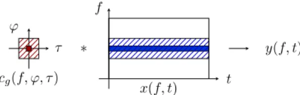
f t τ ϕ cg(f, ϕ, τ ) x(f, t) ∗ y(f, t)
Fig. 2. TF implementation of convolution
focused on the particular case of critically sampled PR cosine modulated filter banks. The general case of stable linear filters is first addressed in Section III-A, then the particular case of stable recursive filters is addressed in Section III-B.
A. Stable linear filters
The PR property of the filter bank implies that the relation-ship betweeny(f, t) and x(f, t) is given by the transformation TTF described in the larger frame in Figure 1(b), where the
input isx(f, t), the output is y(f, t), and transformation TTD
is defined as the time-domain convolution byg(n + N ). The resulting mathematical expression is given in Proposition 1. Proposition 1. Letg(n) ∈ l1(F) be the impulse response of a
stable linear filter, andx(n) ∈ l∞(F) and y(n) ∈ l∞(F) two
signals such that
y(n) = (g ∗ x)(n). (6)
Let y(f, t) and x(f, t) be the TF representations of these
signals as defined in Section II-B. Then
y(f, t) =! ϕ∈Z ! τ ∈Z cg(f, ϕ, τ ) x(f − ϕ, t − τ ) (7) where∀f ∈ [0 . . . F − 1], ∀ϕ ∈ Z, ∀τ ∈ Z, cg(f, ϕ, τ ) = (hf∗ ˜hf −ϕ∗ g)(D(τ + L)), (8)
with the convention∀f /∈ [0 . . . F − 1], hf = 0.
Proof. Firstly, applying equation (3) to signaly yields
y(f, t) = (hf ∗ y)(Dt). (9)
Secondly, equation (4) yields x(n) = F −1! f=0 ! t∈Z ˜ hf(n − D(t − L))x(f, t). (10)
Lastly, equations (7) and (8) are obtained by successively substituting equations (6) and (10) into equation (9).
Remark 1. As mentioned in Section II-B, if |ϕ| ≥ K, then
frequency bandsf and f − ϕ do not overlap, thus cg(f, ϕ, τ )
can be neglected.
Equation (7) shows that a convolution in the original time domain is equivalent to a 2D-convolution in the TF domain, which is stationary w.r.t. time, and non-stationary w.r.t. fre-quency, as illustrated in Figure 2.
B. Stable recursive filters
In this section, we introduce a parametric family of TF filters based on a state space representation, and we show a relationship between these TF filters and equation (7). Definition 1. Stable recursive filtering in TF domain is defined
by the following state space representation:
∀f ∈ [0 . . . F − 1], ∀t ∈ Z, z(f, t) = x(f, t) − Qa " τ=1 ag(f, τ )z(f, t − τ ) y(f, t) = Pb " ϕ=−Pb " τ ∈Z bg(f, ϕ, τ ) z(f − ϕ, t − τ ) (11) whereQa ∈ N, Pb ∈ N, and ∀f ∈ [0 . . . F − 1], x(f, t) ∈
l∞(F) is the sequence of input variables, z(f, t) ∈ l∞(F) is
the sequence of state variables, andy(f, t) ∈ l∞(F) is the
sequence of output variables. The autoregressive parameters
ag(f, τ ) ∈ F define a causal sequence of support [0 . . . Qa]
w.r.t. τ (with ag(f, 0) = 1), having only simple poles
ly-ing inside the unit circle. The movly-ing average parameters
bg(f, ϕ, τ ) ∈ F define a sequence of finite support w.r.t. τ ,
and∀f ∈ [0 . . . F − 1], ∀ϕ ∈ [−Pb. . . Pb], bg(f, ϕ, τ ) = 0
provided thatf − ϕ /∈ [0 . . . F − 1].
Proposition 2. If g(n) ∈ l1(F) is the impulse response of
a causal and stable recursive filter, then the TF input/output system defined in Proposition 1 admits the state space
repre-sentation (11), where Pb = K − 1 and ∀f ∈ [0 . . . F − 1],
∀ϕ ∈ [−Pb, Pb], bg(f, ϕ, τ ) is a sequence of support [−L +
1 . . . − L + 1 + Qb] w.r.t. τ , where Qb≥ 2L + Qa− 1.
Proposition 2 is proved in Appendix A.
Proposition 3. In Definition 1, equation (11) can be rewritten
in the form of equation(7), where∀f ∈ [0 . . . F − 1], ∀τ ∈ Z,
cg(f, ϕ, τ ) = 0 if |ϕ| > Pb, and ∀f ∈ [0 . . . F − 1],
∀ϕ ∈ [−Pb. . . Pb], filter cg(f, ϕ, τ ) is defined as the only
sta-ble (bounded-input, bounded-output) solution of the following recursion: ∀τ ∈ Z, Qa ! t=0 ag(f − ϕ, t)cg(f, ϕ, τ − t) = bg(f, ϕ, τ ). (12)
Proposition 3 is proved in Appendix A.
Remark2. In Definition 1,ag(f, τ ) and bg(f, ϕ, τ ) are
over-parametrised compared to g(n) in Proposition 1. Conse-quently, if the values ofag(f, τ ) and bg(f, ϕ, τ ) are arbitrary,
then it is possible that no filter g(n) exists such that equa-tion (8) holds, which means that this state space representaequa-tion does no longer correspond to a convolution in the original time domain. In this case, we will say that the TF transformation defined in equation (11) is inconsistent2.
2In the TF domain HR-NMF model introduced in Section IV, as well as
in the variational EM algorithm presented in Section V, the consistency of the filter parameters is not explicitly enforced. In practice, the consistency of the estimated parameters will depend on the observed data itself. If the data is clean and informative enough, then the estimated parameters should be consistent. If the data is noisy and poorly informative (for instance in a frequency band where there is no harmonic partial but only noise), then the estimated parameters may not be consistent. However the impact of this discrepancy on the performance might be rather limited in applications.
IV. MULTICHANNELHR-NMFINTFDOMAIN
In this section we present the multichannel HR-NMF model in the TF domain, as initially introduced in [29]. Here this model will be derived from the definition of HR-NMF pro-vided in the time domain in Section II-A.
Following the definition in equation (1), the multichannel HR-NMF model of TF data vm(f, t) ∈ F is defined for all
channelsm ∈ [0 . . . M −1], discrete frequencies f ∈ [0 . . . F − 1], and times t ∈ [0 . . . T − 1], as the sum of S source images yms(f, t) ∈ F plus a 2D-white noise
wm(f, t) ∼ NF(0, σ2w), (13)
whereNF(0, σ2w) denotes a real (if F = R) or circular complex
(if F= C) normal distribution of mean 0 and variance σ2 w: vm(f, t) = wm(f, t) + S−1 ! s=0 yms(f, t). (14)
Then Proposition 2 shows how the convolution in equa-tion (2) can be rewritten in the TF domain: the recursive filtersgms can be accurately implemented via equations (15)
and (17), which come from Definition 13. Each source image
yms(f, t) for s ∈ [0 . . . S − 1] is thus defined as
yms(f, t) = Pb ! ϕ=−Pb Qb ! τ=0 bms(f, ϕ, τ ) zs(f − ϕ, t − τ ) (15) wherePb, Qb∈ N, bms(f, ϕ, τ ) = 0 if f − ϕ /∈ [0 . . . F − 1],
and the latent componentszs(f, t) ∈ F are defined as follows: • ∀t ∈ [−Qz. . . − 1] where Qz= max(Qb, Qa), zs(f, t) ∼ N (µs(f, t), 1/ρs(f, t)), (16) • ∀t ∈ [0 . . . T − 1], zs(f, t) = xs(f, t) − Qa ! τ=1 as(f, τ )zs(f, t − τ ) (17) where xs(f, t) ∼ NF(0, σ2xs(t)), Qa ∈ N and as(f, τ )
defines a stable autoregressive filter.
Note that the variance σ2xs(t) of xs(f, t) does not depend on
frequency f . This particular choice allows us to make the model identifiable, as suggested in Section II-A (the variability w.r.t. frequency is already modelled via the the filtersgms).
The random variables wm(f1, t1) and xs(f2, t2) for all
s, m, f1, f2, t1, t2 are assumed mutually independent.
Addi-tionally, ∀m ∈ [0 . . . M − 1], ∀f ∈ [0 . . . F − 1], ∀t ∈ [−Qz. . . − 1], vm(f, t) is unobserved, and ∀s ∈ [0 . . . S − 1],
the prior meanµs(f, t) ∈ F and the prior precision (inverse
variance) ρs(f, t) > 0 of the latent variable zs(f, t) are
considered to be fixed parameters.
The set θ of parameters to be estimated consists of:
• the autoregressive parameters as(f, τ ) ∈ F for s ∈
[0 . . . S − 1], f ∈ [0 . . . F − 1], τ ∈ [1 . . . Qa] (we further
defineas(f, 0) = 1),
3More precisely, compared to the result of Proposition 2, processes z s(f, t)
and xs(f, t) as defined in Section IV are shifted L − 1 samples backward, in
order to write bms(f, ϕ, τ ) in a causal form. This does not alter the definition
of HR-NMF, since equation (17) is unaltered by this time shift, and yms(f, t)
• the moving average parameters bms(f, ϕ, τ ) ∈ F for
m ∈ [0 . . . M − 1], s ∈ [0 . . . S − 1], f ∈ [0 . . . F − 1], ϕ∈ [−Pb. . . Pb], and τ ∈ [0 . . . Qb],
• the variance parameters σw2 > 0 and σx2s(t) > 0 for
s ∈ [0 . . . S − 1] and t ∈ [0 . . . T − 1]. We thus have θ= {σ2
w, σx2s, as, bms}s∈[0...S−1],m∈[0...M−1].
This model encompasses the following special cases:
• IfM = 1, σ2
w = 0 and Pb= Qb= Qa= 0, then
equa-tion (14) reduces tov0(f, t) ="S−1s=0 b0s(f, 0, 0)xs(f, t),
thus v0(f, t) ∼ NF(0, #Vf t), where matrix #V of
co-efficients #Vf t is defined by the NMF #V = W H
with Wf s = |b0s(f, 0, 0)|2 and Hst = σx2s(t). The
maximum likelihood estimation of W and H is then equivalent to the minimization of the Itakura-Saito (IS) divergence between matrix #V and spectrogram V (where Vf t= |v0(f, t)|2), hence this model is referred to as
IS-NMF [14].
• If M = 1 and Pb = Qb = 0, then v0(f, t) follows the
monochannel HR-NMF model [25], [26], [31] involving variance σ2w, autoregressive parameters as(f, τ ) for all
s ∈ [0 . . . S − 1], f ∈ [0 . . . F − 1] and τ ∈ [1 . . . Qa],
and the NMF #V = W H.
• IfS = 1, σw2 = 0, Pb= 0, σ2x0(t) = 1 ∀t ∈ [0 . . . T − 1],
andµs(f, t) = 0 and ρs(f, t) = 1 ∀t ∈ [−Qz. . . − 1],
then∀m ∈ [0 . . . M − 1], ∀f ∈ [0 . . . F − 1], vm(f, t) is
an autoregressive moving average (ARMA) process [27, Section 3.6].
• IfS = 1, σ2
w= 0, Pb= 0, Qa> 0, Qb= Qa− 1, ∀t ∈
[−Qz. . . − 1], µ0(f, t) = 0, ρ0(f, t) ) 1, and σ2x0(t) =
{t=0}(where S denotes the indicator function of a set
S), then ∀m ∈ [0 . . . M − 1], ∀f ∈ [0 . . . F − 1], vm(f, t)
can be written in the formvm(f, t) ="Qτ=1a αmτzτ(f )t,
where z1(f ) . . . zQa(f ) are the roots of the polynomial
zQa +"Qa
τ=1a0(f, τ )zQa−τ. This corresponds to the
Exponential Sinusoidal Model (ESM) commonly used in HR spectral analysis of time series [27], [32]. Because it generalizes both IS-NMF and ESM models to multichannel data, the model defined in equation (14) is called multichannel HR-NMF.
V. VARIATIONALEMALGORITHM
In early works that focused on monochannel HR-NMF [25], [26], in order to estimate the model parameters we proposed to resort to an expectation-maximization (EM) algorithm based on a Kalman filter/smoother. The approach proved to be appropriate for modelling audio signals in applications such as source separation and audio inpainting. However, its computa-tional cost was high, dominated by the Kalman filter/smoother, and prohibitive when dealing with high-dimensional signals.
In order to make the estimation of HR-NMF faster, we then proposed two different strategies. The first approach aimed to improve the convergence rate, by replacing the M-step of the EM algorithm by multiplicative update rules [33]. However we observed that the resulting algorithm presented some
nu-merical stability issues4. The second approach aimed to reduce
the computational cost, by using a variational EM algorithm, where we introduced two different variational approxima-tions [31]. We observed that the mean field approximation led to both improved performance and maximal decrease of computational complexity.
In this section, we thus generalize the variational EM algorithm based on mean field approximation to the multichan-nel HR-NMF model introduced in Section IV, as proposed in [29]. Compared to [31], novelties also include a reduced computational complexity and a parallel implementation.
A. Review of variational EM algorithm
Variational inference [34] is now a classical approach for estimating a probabilistic model involving both observed vari-ables v and latent variables z, determined by a set θ of parameters. Let F be a set of probability density functions (PDFs) over the latent variablesz. For any PDF q ∈ F and any function φ(z), we note ⟨φ⟩q = $φ(z)q(z)dz. Then for
any set of parameters θ, the variational free energy is defined as L(q; θ) = % ln & p(v, z; θ) q(z) '( q . (18) The variational EM algorithm is a recursive algorithm for estimating θ. It consists of the two following steps at each iterationi:
• Expectation (E)-step (updateq): q⋆= argmax
q∈F
L(q; θi−1) (19) • Maximization (E)-step (update θ):
θi= argmax θ
L(q⋆
; θ). (20) In the case of multichannel HR-NMF, θ has been specified in Section IV. We further define δm(f, t) = 1 if vm(f, t) is
observed, otherwise δm(f, t) = 0, in particular δm(f, t) = 0
∀(f, t) /∈ [0 . . . F − 1] × [0 . . . T − 1]. The complete set of variables consists of:
• the set v of observed variables vm(f, t) for m ∈
[0 . . . M − 1] and for all f and t such that δm(f, t) = 1, • the setz of latent variables zs(f, t) for s ∈ [0 . . . S − 1],
f ∈ [0 . . . F − 1], and t ∈ [−Qz. . . T − 1].
We use a mean field approximation [34]:F is defined as the set of PDFs which can be factorized in the form
q(z) = S−1) s=0 F −1) f=0 T −1) t=−Qz qsf t(zs(f, t)). (21) 4Indeed, the convergence of multiplicative update rules was not proved
in [33] (more specifically, there is no theoretical guarantee that the log-likelihood is non-decreasing), whereas the convergence of EM strategies is well established. Besides, as stated in [33], we observed that multiplicative update rules may exhibit some numerical instabilities for small values of the tuning parameter # (the variation of the log-likelihood oscillates instead of monotonically increasing), which was the reason for introducing a more stable tempering approach, that consists in making ε vary from 1 to a lower value over iterations. In this paper, we therefore preferred to use a slower method with guaranteed convergence. It is possible that the convergence rate could be improved in future using multiplicative update rules.
With this particular factorization ofq(z), the solution of (19) is such that each PDFqsf t is Gaussian:
zs(f, t) ∼ NF(zs(f, t), γzs(f, t)).
In the following sections, we will use notation φ= ⟨φ⟩q and
γφ= ⟨|φ − φ|2⟩q, for any function φ of the latent variables.
B. Variational free energy
Let α = 1 if F = C, and α = 2 if F = R. Let Dv = M −1" m=0 F −1" f=0 T −1" t=0
δm(f, t) be the number of observations, and
I(f, t) = {0≤f <F, 0≤t<T }, evm(f, t) = δm(f, t) & vm(f, t) − S−1" s=0 yms(f, t) ' , xs(f, t) = I(f, t) * Q"a τ=0 as(f, τ )zs(f, t − τ ) + . Then using equations (13) to (16), the joint log-probability distribution L = log(p(v, z; θ)) of the complete set of vari-ables satisfies −αL = −α (ln(p(v|z; θ)) + ln(p(z; θ))) = (Dv+ SF (T + Qz)) ln(απ) +Dvln(σ2w) +σ12 w M −1" m=0 F −1" f=0 T −1" t=0 |evm(f, t)| 2 +S−1" s=0 F −1" f=0 −1 " t=−Qz ln( 1 ρs(f,t)) +S−1" s=0 F −1" f=0 −1 " t=−Qz ρs(f, t)|zs(f, t) − µs(f, t)|2 +S−1" s=0 F −1" f=0 T −1" t=0 ln(σ2 xs(t)) + 1 σ2 xs(t)|xs(f, t)| 2 . Thus the variational free energy defined in (18) satisfies −αL = Dvln(απ) − SF (T + Qz) +Dvln(σ2w) + M −1" m=0 F −1" f=0 T −1" t=0 γevm(f,t)+|evm(f,t)|2 σ2 w +S−1" s=0 F −1" f=0 −1 " t=−Qz − ln(ρs(f, t)γzs(f, t)) +ρs(f, t) , γzs(f, t) + |zs(f, t) − µs(f, t)|2 -+S−1" s=0 F −1" f=0 T −1" t=0 ln* σ 2 xs(t) γzs(f,t) + +γxs(f,t)+|xs(f,t)|2 σ2 xs(t) (22) where∀f ∈ [0 . . . F − 1], ∀t ∈ [0 . . . T − 1], γevm(f, t) = δm(f, t) S−1" s=0 γyms(f, t), γyms(f, t) = Pb " ϕ=−Pb Qb " τ=0 |bms(f, ϕ, τ )|2γzs(f − ϕ, t − τ ), evm(f, t) = δm(f, t) & vm(f, t) − S−1" s=0 yms(f, t) ' , yms(f, t) = Pb " ϕ=−Pb Qb " τ=0 bms(f, ϕ, τ ) zs(f − ϕ, t − τ ), γxs(f, t) = I(f, t) * Q"a τ=0 |as(f, τ )|2γzs(f, t − τ ) + , xs(f, t) = I(f, t) *Q"a τ=0 as(f, τ )zs(f, t − τ ) + .
C. Variational EM algorithm for multichannel HR-NMF
According to the mean field approximation, the maximiza-tions in equamaximiza-tions (19) and (20) are performed for each scalar parameter in turn [34]. The dominant complexity of each iteration of the resulting variational EM algorithm is 4M F ST ∆f ∆t, where ∆f = 1 + 2Pband∆t = 1 + Qz (by
updating the model parameters in turn rather than jointly, the complexity of the M-step has been divided by a factor(∆t)2
compared to [31]). However we highlight a possible parallel implementation, by making a difference between parfor loops which can be implemented in parallel, and for loops which have to be implemented sequentially.
1) E-step: For all s ∈ [0 . . . S − 1], f ∈ [0 . . . F − 1],
t /∈ [−Qz, −1], let ρs(f, t) = 0. Considering the mean
field approximation (21), the E-step defined in equation (19) leads to the updates described in Table I (where ∗ denotes complex conjugation). Note that zs(f, t) has to be updated
after γzs(f, t).
2) M-step: The M-step defined in (20) leads to the updates
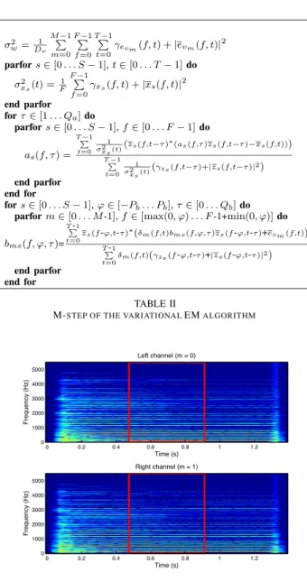
described in Table II. The updates of the four parameters can be processed in parallel. parfors∈ [0 . . . S − 1], f ∈ [0 . . . F − 1], t ∈ [−Qz. . . T− 1] do γzs(f, t)−1= ρs(f, t) + Qa ! τ=0 I(f,t+τ )|as(f,τ )|2 σ2 xs(t+τ ) + M−1 ! m=0 Pb ! ϕ=−Pb Qb ! τ=0 δm(f +ϕ,t+τ )|bms(f +ϕ,ϕ,τ )|2 σ2 w end parfor fors∈ [0 . . . S-1], f0∈ [0 . . . ∆f-1], t0∈ [-Qz. . .-Qz+∆t-1] do parfor f−f0 ∆f ∈ [0 . . . ⌊ F−1−f0 ∆f ⌋], t−t0 ∆t ∈ [0 . . . ⌊ T−1−t0 ∆t ⌋] do zs(f, t) = zs(f, t) − γzs(f, t) " ρs(f, t)(zs(f, t) − µs(f, t)) + Qa ! τ=0 as(f,τ )∗xs(f,t+τ ) σ2 xs(t+τ ) − M−1 ! m=0 Pb ! ϕ=−Pb Qb ! τ=0 bms(f +ϕ,ϕ,τ )∗evm(f +ϕ,t+τ ) σ2 w # end parfor end for TABLE I
E-STEP OF THE VARIATIONALEMALGORITHM
VI. SIMULATION RESULTS
In this section, we present a basic proof of concept of the multichannel HR-NMF model. The ability to accurately model reverberation and restore missing observations is illustrated in Section VI-A, and the ability to separate pure tones with close frequencies is illustrated in Section VI-B.
A. Audio inpainting
The following experiments deal with a single source (S = 1) formed of a real piano sound sampled at11025 Hz. A 1.25ms-short stereophonic signal (M = 2) has been synthesized by fil-tering the monophonic recording of a loud C3 piano note from the MUMS database [35] with two room impulse responses
σ2w=D1 v M−1 ! m=0 F−1 ! f=0 T−1 ! t=0 γevm(f, t) + |evm(f, t)| 2 parfors∈ [0 . . . S − 1], t ∈ [0 . . . T − 1] do σ2xs(t) =F1 F−1 ! f=0 γxs(f, t) + |xs(f, t)| 2 end parfor for τ∈ [1 . . . Qa] do parfors∈ [0 . . . S − 1], f ∈ [0 . . . F − 1] do as(f, τ ) = T −1! t=0 1 σ2 xs (t)( zs(f,t−τ )∗(as(f,τ )zs(f,t−τ )−xs(f,t))) T −1! t=0 1 σ2 xs(t)( γzs(f,t−τ )+|zs(f,t−τ )|2) end parfor end for fors∈ [0 . . . S − 1], ϕ ∈ [−Pb. . . Pb], τ ∈ [0 . . . Qb] do
parform∈ [0 . . . M -1], f ∈ [max(0, ϕ) . . . F -1+min(0, ϕ)] do bms(f, ϕ, τ )= T!-1 t=0zs(f-ϕ,t-τ) ∗(δm(f,t)bms(f,ϕ,τ )zs(f-ϕ,t-τ)+e vm(f,t)) T!-1 t=0 δm(f,t)(γzs(f-ϕ,t-τ)+|zs(f-ϕ,t-τ)|2) end parfor end for TABLE II
M-STEP OF THE VARIATIONALEMALGORITHM
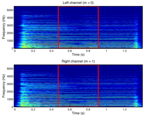
Time (s) Frequency (Hz) Left channel (m = 0) 0 0.2 0.4 0.6 0.8 1 1.2 0 1000 2000 3000 4000 5000 Time (s) Frequency (Hz) Right channel (m = 1) 0 0.2 0.4 0.6 0.8 1 1.2 0 1000 2000 3000 4000 5000
Fig. 3. Input stereo signal vm(f, t).
simulated using the Matlab code presented in [36]5. The TF
representationvm(f, t) of this signal has then been computed
by applying a critically sampled PR cosine modulated filter bank (F= R) with F = 201 frequency bands, involving filters of length8F = 1608 samples. The resulting TF representation, of dimensionF × T with T = 77, is displayed in Figure 3. In particular, it can be noticed that the two channels are not synchronous (the starting time in the left channel is≈ 0.04s, whereas it is≈ 0.02s in the right channel), which suggests that the orderQbof filters bms(f, ϕ, τ ) should be chosen greater
than zero.
In the following experiments, we have setµs(f, t) = 0 and
ρs(f, t) = 105. These values force zs(f, t) to be close to
zero∀t ∈ [−Qz. . . − 1] (since the prior mean and variance 5Those impulse responses were simulated using 15625 virtual sources. The
dimensions of the room were [20m, 19m, 21m], the coordinates of the two microphones were [19m, 18m 1.6m] and [15m, 11m, 10m], and those of the source were [5m, 2m, 1m]. The reflection coefficient of the walls was 0.3.
ofzs(f, t) are µs(f, t) = 0 and 1/ρs(f, t) = 10−5), which
is relevant if the observed sound is preceded by silence. The variational EM algorithm is initialized with the neutral values zs(f, t) = 0, γzs(f, t) = σ
2
w = σ2xs(t) = 1,
as(f, τ ) = {τ =0}, and bms(f, ϕ, τ ) = {ϕ=0,τ =0}. In order
to illustrate the capability of the multichannel HR-NMF model to synthesize realistic audio data, we address the case of missing observations. We suppose that all TF points within the red frame in Figure 3 are unobserved: δm(f, t) = 0
∀t ∈ [26 . . . 50] (which corresponds to the time range 0.47s-0.91s), and δm(f, t) = 1 for all other t in [0 . . . T − 1]. In each
experiment, 100 iterations of the algorithm are performed, and the restored signal is returned asyms(f, t).
In the first experiment, a multichannel HR-NMF with Qa = Qb = Pb = 0 is estimated. Similarly to the example
provided in Section IV, this is equivalent to modelling the two channels by two rank-1 IS-NMF models [14] having distinct spectral atoms W and sharing the same temporal activation H, or by a rank 1 multichannel NMF [23]. The resulting TF representation yms(f, t) is displayed in Figure 4. It can be
noticed that wherever vm(f, t) is observed (δm(f, t) = 1),
yms(f, t) does not accurately fit vm(f, t) (this is particularly
visible in high frequencies), because the lengthQb of filters
bms(f, ϕ, τ ) has been underestimated: the source to distortion
ratio (SDR)6in the observed area is11.7dB. In other respects, the missing observations (δm(f, t) = 0) could not be restored
(yms(f, t) is zero inside the frame, resulting in an SDR of 0dB
in this area), because the correlations between contiguous TF coefficients invm(f, t) have not been taken into account.
Time (s) Frequency (Hz) Left channel (m = 0) 0 0.2 0.4 0.6 0.8 1 1.2 0 1000 2000 3000 4000 5000 Time (s) Frequency (Hz) Right channel (m = 1) 0 0.2 0.4 0.6 0.8 1 1.2 0 1000 2000 3000 4000 5000
Fig. 4. Stereo signal yms(f, t) estimated with filters of length 1.
In the second experiment, a multichannel HR-NMF model withQa= 2, Qb= 3, and Pb= 1 is estimated. The resulting
TF representationyms(f, t) is displayed in Figure 5. It can be
noticed that wherever vm(f, t) is observed, yms(f, t) better
fitsvm(f, t): the SDR is 36.8dB in the observed area. Besides,
the missing observations have been better estimated: the SDR is 4.8dB inside the frame. Actually, choosing Pb > 0 was 6The SDR between a data vector v and an estimate v is defined asˆ
20 log10
" ∥v∥
2 ∥v−ˆv∥2
#
necessary to obtain this result, which means that the spectral overlap between frequency bands cannot be neglected in this multichannel setting. Time (s) Frequency (Hz) Left channel (m = 0) 0 0.2 0.4 0.6 0.8 1 1.2 0 1000 2000 3000 4000 5000 Time (s) Frequency (Hz) Right channel (m = 1) 0 0.2 0.4 0.6 0.8 1 1.2 0 1000 2000 3000 4000 5000
Fig. 5. Stereo signal yms(f, t) estimated with longer filters.
B. Source separation
In this section, we aim to illustrate the ability of HR-NMF to separate pure tones with close frequencies, based on the autoregressive parameters as(f, τ ), in a difficult
underdeter-mined setting (M < S)7. For simplicity, we have chosen to
deal with a2s-long monophonic mixture (M = 1), composed of a chord of S = 2 piano notes, one semitone apart (A4 and Ab4 from the MAPS database [37]8, whose fundamental
frequencies are 440 Hz and 415.30 Hz), resampled at8600 Hz. The TF representation v0(f, t) of this mixture signal was
computed via an STFT (F= C), involving 90 ms-long Hann windows with 75% overlap,F = 400 frequency bands and T = 87 time frames. Here the full TF representation displayed in Figure 6 is observed (δ0(f, t) = 1). In this experiment,
we compare the signals separated by means of the HR-NMF model in two configurations. In the first configuration, Qa = Qb = Pb = 0 and σ2w = 0, which means that
each source follows a rank-1 IS-NMF model. In the second configuration,Qa= 1 and Qb= Pb= 0, which permits us to
accurately model pure tones by means of the autoregressive parametersas(f, τ ).
Contrary to the monophonic case (S = 1) addressed in Section VI-A, applying the variational EM to multiple sources (S > 1) in a fully unsupervised way is difficult: except in some simple settings such as Qa = Qb = Pb = 0, the
algorithm hardly converges to a relevant solution, possibly because of a higher number of local maxima in the variational free energy. Nevertheless, separation of multiple sources is still feasible in a semi-supervised situation, where some parameters are learned beforehand. Here the spectral parametersas(f, τ ) 7In a similar experiment involving a determined multichannel setting (M=
S= 2), the spatial information proved to be sufficient to accurately separate the two tones, without even using autoregressive parameters (Qa= 0).
8MAPS database, ISOL set, ENSTDkCl instrument, mezzo-forte loudness,
with the sustain pedal.
Fig. 6. Spectrogram of the mixture of the A4 and Ab4 piano notes.
and bms(f, ϕ, τ ) are thus estimated in a first stage from
the original source signals. In the first configuration, the values of all NMF parameters are initialized to 1, and 30 iterations of multiplicative update rules [14] are performed. In the second configuration, the variational EM algorithm is initialized with µs(f, t) = 0, ρs(f, t) = 105, zs(f, t) = 0,
γzs(f, t) = 1, as(f, τ ) = {τ =0},bms(f, ϕ, τ ) = {ϕ=0,τ =0},
σ2
w= σx2s(t) = 1, and 100 iterations are performed.
In a second stage, the variance parameters σ2
xs(t) and σ
2 w
are estimated from the observed mixture, and the separated signals are obtained as y0s(f, t) for s ∈ {0, 1}. In the first configuration, the spectral parameters learned in the first stage are kept unchanged, the values of the time activations σ2
xs(t)
are initialized to 1, and 30 iterations of multiplicative update rules are performed. In the second configuration, the spectral parameters learned in the first stage are kept unchanged, the variational EM algorithm is initialized with the time activations σx2s(t) estimated in the first configuration, the
value σ2w = 10−2, and the same initial values of the other
parameters as in the first stage. Then 100 iterations of the E-step are performed in order to let zs(f, t) and γzs(f, t)
converge to relevant values based on the learned parameters, and finally 100 iterations of the full variational EM algorithm are performed.
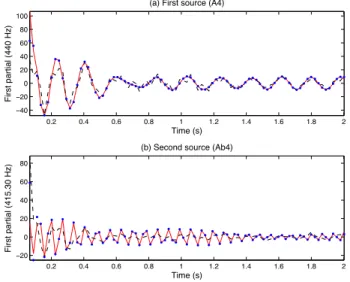
In order to assess the separation performance, we have evaluated the SDR obtained in the two configurations. In the first configuration, the SDR of A4 is 17.67 dB and that of Ab4 is 23.08 dB. In the second configuration, the SDR of A4 is increased to 22.37 dB and that of Ab4 is increased to 27.78 dB. Figure 7 focuses on the results obtained in the frequency bandf = 40, where the first partials of A4 and Ab4 overlap, resulting in a challenging separation problem. The real parts of the original sources are represented as red solid lines. As expected, the two sources are not properly separated in the first configuration (IS-NMF), because the estimated signals (represented as black dashed lines) are obtained by multiplying the mixture signal by a nonnegative mask, and interferences cannot be cancelled. As a comparison, the signals estimated in the second configuration (represented as blue dots) accurately
fit the partials of the original sources. Note however that this remarkable result was obtained by guiding the variational EM algorithm with relevant initial values. In future work, we will need to develop robust estimation methods, less sensitive to initialisation, in order to perform source separation in a fully unsupervised way. 0.2 0.4 0.6 0.8 1 1.2 1.4 1.6 1.8 2 −40 −20 0 20 40 60 80 100 Time (s) First partial (440 Hz)
(a) First source (A4)
0.2 0.4 0.6 0.8 1 1.2 1.4 1.6 1.8 2 −20 0 20 40 60 80 Time (s) First partial (415.30 Hz)
(b) Second source (Ab4)
Fig. 7. Separation of two sinusoidal components. The real parts of the two components y0s(f, t) are plotted as red solid lines, their IS-NMF estimates
are plotted as black dashed lines, and their HR-NMF estimates are plotted as blue dots.
VII. CONCLUSIONS
In this paper, we have shown that convolution can be accurately implemented in the TF domain, by applying 2D-filters to a TF representation obtained as the output of a PR filter bank. In the particular case of recursive filters, we have also shown that filtering can be implemented by means of a state space representation in the TF domain. These results have then been used to extend the monochannel HR-NMF model initially proposed in [25], [26] to multichannel signals and convolutive mixtures. The resulting multichannel HR-NMF model can accurately represent the transfer from each source to each sensor, as well as the spectrum of each source. It also takes the correlations over frequencies into account. In order to estimate this model from real audio data, a variational EM algorithm has been proposed, which has a re-duced computational complexity and a parallel implementation compared to [31]. This algorithm has been successfully applied to piano signals, and has been capable of accurately modelling reverberation due to room impulse response, restoring missing observations, and separating pure tones with close frequencies. In order to deal with more realistic music signals, the esti-mation of the HR-NMF model should be performed in a more informed way, e.g. by means of semi-supervised learning, or by using any kind of prior information about the mixture or about the sources. For instance, harmonicity and temporal or spectral smoothness could be enforced by re-parametrising the model, or by introducing some prior distributions of the model
parameters. Because audio signals are sparse in the time-frequency domain, we observed that the multichannel HR-NMF model involves a small number of non-zero parameters in practice. In future work, we will investigate enforcing this property, by introducing a prior distribution of the filter parameters such as that proposed in [38], or a prior distribution of the variances of the innovation processxs(f, t) (modelling
variances with a prior distribution is an idea that has been successfully investigated in earlier works [39]–[41]). In other respects, the model could also be extended in several ways, for instance by taking the correlations over latent components into account, or by using other types of TF transforms, e.g. wavelet transforms.
Regarding the estimation of the HR-NMF model, the mean field approximation involved in our variational EM algorithm is known to induce a slow convergence rate. The convergence could thus be accelerated by replacing the mean field ap-proximation by a structured mean field apap-proximation, like in [42]. Such an approximation was already proposed to esti-mate the monochannel HR-NMF model [31], at the expense of a higher computational complexity per iteration. Some alternative Bayesian estimation techniques such as Markov chain Monte Carlo (MCMC) methods and message passing algorithms [34] could also be applied to the HR-NMF model. In other respects, we observed that the variational EM algo-rithm is hardly able to separate multiple concurrent sources in a fully unsupervised framework, because of its high sensitivity to initialisation. More robust estimation methods are thus needed, which could for instance take advantage of the algebra principles exploited in high resolution methods [32].
Lastly, the multichannel HR-NMF model could be used in a variety of applications, such as source coding, audio inpaint-ing, automatic music transcription, and source separation.
APPENDIX
TFIMPLEMENTATION OF STABLE RECURSIVE FILTERING
Proof of Proposition 2. We consider the TF implementation
of convolution given in Proposition 1, and we defineg(n) as the impulse response of a causal and stable recursive filter, having only simple poles. Then the partial fraction expansion of its transfer function [43] shows that it can be written in the formg(n) = g0(n) +"Qk=1gk(n), where Q ∈ N, g0(n) is a
causal sequence of support[0 . . . N0− 1] (with N0∈ N), and
∀k ∈ [1 . . . Q],
gk(n) = βkeδkncos(2πνkn + ψk) n≥0
where βk> 0, δk< 0, νk∈ [0,12], ψk∈ R.
Then∀f ∈ [0 . . . F − 1], equation (8) yields cg(f, ϕ, τ ) =
"Q k=0cgk(f, ϕ, τ ) with cg0(f, ϕ, τ ) = (hf ∗ ˜hf −ϕ∗ g0)(D(τ + L)) and∀k ∈ [1 . . . Q], cgk(f, ϕ, τ ) = e δkDτ(A k(f, ϕ, τ ) cos(2πνkDτ ) +Bk(f, ϕ, τ ) sin(2πνkDτ ))
where we have defined Ak(f, ϕ, τ ) = βk N −1" n=−N +1 (hf∗ ˜hf −ϕ)(n + N ) ×e−δkncos(2πν kn − ψk) n≤Dτ, Bk(f, ϕ, τ ) = βk"N −1n=−N +1(hf∗ ˜hf −ϕ)(n + N ) ×e−δknsin(2πν kn − ψk) n≤Dτ.
It can be easily proved that∀f ∈ [0 . . . F − 1], ∀ϕ ∈ Z,
• the support ofcg0(f, ϕ, τ ) is [−L + 1 . . . L + ⌈
N0−2
D ⌉], • if τ≤ −L, then cg0(f, ϕ, τ ), Ak(f, ϕ, τ ) and Bk(f, ϕ, τ )
are zero, thuscg(f, ϕ, τ ) = 0,
• if τ≥ L, then Ak(f, ϕ, τ ) and Bk(f, ϕ, τ ) do not depend
on τ .
Therefore∀f ∈ [0 . . . F − 1], ∀ϕ ∈ Z, cg(f, ϕ, τ − L + 1)
is the impulse response of a causal and stable recursive filter, whose transfer function has a denominator of order2Q and a numerator of order2L + 2Q − 1 + ⌈N0−2
D ⌉].
As a particular case, suppose that∀k ∈ [1 . . . Q], |δk| / 1.
If τ≥ L, then Ak(f, ϕ, τ ) and Bk(f, ϕ, τ ) can be neglected
as soon as νk does not lie in the supports of both Hf(ν)
andHf −ϕ(ν), where Hf was defined in equation (5). Thus
for each f and ϕ, there is a limited number Q(f, ϕ) ≤ Q (possibly 0) of cgk(f, ϕ, τ ) which contribute to cg(f, ϕ, τ ).
In the general case, we can still consider without loss of generality that ∀f ∈ [0 . . . F − 1], ∀ϕ ∈ Z, there is a limited numberQ(f, ϕ) ≤ Q of cgk(f, ϕ, τ ) which contribute
to cg(f, ϕ, τ ). We then define Qa = 2max
f,ϕ Q(f, ϕ) and
Qb = 2L + Qa− 1 + ⌈N0D−2⌉. Then ∀f ∈ [0 . . . F − 1],
∀ϕ ∈ Z, cg(f, ϕ, τ − L + 1) is the impulse response of
a causal and stable recursive filter, whose transfer function has a denominator of order Qa and a numerator of order
Qb. Considering Remark 1, we conclude that the input/output
system described in equation (7) is equivalent to the state space representation (11), wherePb= K − 1.
Proof of Proposition 3. We consider the state space
repre-sentation in Definition 1, and we first assume that ∀f ∈ [0 . . . F − 1], sequences x(f, t), y(f, t), and z(f, t) belong to l1(Z). Then the following DTFTs are well-defined:
Y (f, ν) = "t∈Zy(f, t)e−2iπνt,
X(f, ν) = "t∈Zx(f, t)e−2iπνt,
Bg(f, ϕ, ν) = "τ ∈Zbg(f, ϕ, τ )e−2iπντ,
Ag(f, ν) = "Qτ=0a ag(f, τ )e−2iπντ.
Then applying the DTFT to equation (11) yieldsZ(f, ν) =
1 Ag(f,ν)X(f, ν) and Y (f, ν) = Pb " ϕ=−Pb Bg(f, ϕ, ν)Z(f − ϕ, ν). Therefore Y (f, ν) = Pb ! ϕ=−Pb Cg(f, ϕ, ν)X(f − ϕ, ν), (23) where Cg(f, ϕ, ν) = Bg(f, ϕ, ν) Ag(f − ϕ, ν) (24)
is the frequency response of a recursive filter. Since this frequency response is twice continuously differentiable, then this filter is stable, which means that its impulse response cg(f, ϕ, τ ) = $01Cg(f, ϕ, ν)e+2iπντdν belongs to l1(F).
Equations (7) and (12) are then obtained by applying an inverse DTFT to (23) and (24). Finally, even ifx(f, t), y(f, t), and z(f, t) belong to l∞(Z) but not to l1(Z), equations (7)
and (11) are still well-defined, and the same filtercg(f, ϕ, τ ) ∈
l1(F) is still the only stable solution of equation (12). ACKNOWLEDGMENT
The authors would like to thank the anonymous reviewers for their very helpful suggestions. This work was undertaken while Roland Badeau was visiting the Centre for Digital Mu-sic, partly funded by EPSRC Platform Grant EP/K009559/1. Mark D. Plumbley is funded by EPSRC Leadership Fellowship EP/G007144/1.
REFERENCES
[1] D. D. Lee and H. S. Seung, “Learning the parts of objects by non-negative matrix factorization,” Nature, vol. 401, pp. 788–791, Oct. 1999. [2] S. A. Raczy´nski, N. Ono, and S. Sagayama, “Multipitch analysis with harmonic nonnegative matrix approximation,” in Proc. 8th International
Society for Music Information Retrieval Conference (ISMIR), Vienna, Austria, Sep. 2007, 6 pages.
[3] P. Smaragdis, “Relative pitch tracking of multiple arbitrary sounds,”
Journal of the Acoustical Society of America (JASA), vol. 125, no. 5, pp. 3406–3413, May 2009.
[4] E. Vincent, N. Bertin, and R. Badeau, “Adaptive harmonic spectral de-composition for multiple pitch estimation,” IEEE Trans. Audio, Speech,
Lang. Process., vol. 18, no. 3, pp. 528–537, Mar. 2010.
[5] P. Smaragdis and J. C. Brown, “Non-negative matrix factorization for polyphonic music transcription,” in Proc. IEEE Workshop on
Applica-tions of Signal Processing to Audio and Acoustics (WASPAA), New Paltz, New York, USA, Oct. 2003, pp. 177–180.
[6] N. Bertin, R. Badeau, and E. Vincent, “Enforcing harmonicity and smoothness in Bayesian non-negative matrix factorization applied to polyphonic music transcription,” IEEE Trans. Audio, Speech, Lang.
Process., vol. 18, no. 3, pp. 538–549, Mar. 2010.
[7] A. Cichocki, R. Zdunek, A. H. Phan, and S.-I. Amari, Nonnegative
Matrix and Tensor Factorizations: Applications to Exploratory Multi-way Data Analysis and Blind Source Separation. Wiley, Nov. 2009. [8] T. Virtanen, “Monaural sound source separation by nonnegative matrix
factorization with temporal continuity and sparseness criteria,” IEEE
Trans. Audio, Speech, Lang. Process., vol. 15, no. 3, pp. 1066–1074, Mar. 2007.
[9] D. FitzGerald, M. Cranitch, and E. Coyle, “Extended nonnegative tensor factorisation models for musical sound source separation,”
Computa-tional Intelligence and Neuroscience, vol. 2008, pp. 1–15, May 2008, article ID 872425.
[10] A. Liutkus, R. Badeau, and G. Richard, “Informed source separation using latent components,” in Proc. 9th International Conference on
Latent Variable Analysis and Signal Separation (LVA/ICA), Saint Malo, France, Sep. 2010, pp. 498–505.
[11] M. N. Schmidt and H. Laurberg, “Non-negative matrix factorization with Gaussian process priors,” Computational Intelligence and Neuroscience, 2008, Article ID 361705, 10 pages.
[12] P. Smaragdis, “Probabilistic decompositions of spectra for sound separa-tion,” in Blind Speech Separation, S. Makino, T.-W. Lee, and H. Sawada, Eds. Springer, 2007, pp. 365–386.
[13] T. Virtanen, A. Cemgil, and S. Godsill, “Bayesian extensions to non-negative matrix factorisation for audio signal modelling,” in Proc. IEEE
International Conference on Acoustics, Speech and Signal Processing (ICASSP), Las Vegas, Nevada, USA, Apr. 2008, pp. 1825–1828. [14] C. F´evotte, N. Bertin, and J.-L. Durrieu, “Nonnegative matrix
factor-ization with the Itakura-Saito divergence. With application to music analysis,” Neural Computation, vol. 21, no. 3, pp. 793–830, Mar. 2009. [15] J. Le Roux and E. Vincent, “Consistent Wiener filtering for audio source separation,” IEEE Signal Process. Lett., vol. 20, no. 3, pp. 217–220, Mar. 2013.
[16] D. Griffin and J. Lim, “Signal reconstruction from short-time Fourier transform magnitude,” IEEE Trans. Acoust., Speech, Signal Process., vol. 31, no. 4, pp. 986–998, Aug. 1983.
[17] J. Le Roux, H. Kameoka, N. Ono, and S. Sagayama, “Fast signal reconstruction from magnitude STFT spectrogram based on spectrogram consistency,” in Proc. 13th International Conference on Digital Audio
Effects (DAFx), Graz, Austria, Sep. 2010, pp. 397–403.
[18] A. Ozerov, C. F´evotte, and M. Charbit, “Factorial scaled hidden Markov model for polyphonic audio representation and source separation,” in
Proc. IEEE Workshop on Applications of Signal Processing to Audio and Acoustics (WASPAA), New Paltz, New York, USA, Oct. 2009, pp. 121–124.
[19] O. Dikmen and A. T. Cemgil, “Gamma Markov random fields for audio source modeling,” IEEE Trans. Audio, Speech, Lang. Process., vol. 18, no. 3, pp. 589–601, Mar. 2010.
[20] G. Mysore, P. Smaragdis, and B. Raj, “Non-negative hidden Markov modeling of audio with application to source separation,” in Proc.
9th international Conference on Latent Variable Analysis and Signal Separation (LCA/ICA), St. Malo, France, Sep. 2010, 8 pages. [21] H. Kameoka, N. Ono, K. Kashino, and S. Sagayama, “Complex NMF:
A new sparse representation for acoustic signals,” in Proc. IEEE
International Conference on Acoustics, Speech and Signal Processing (ICASSP), Taipei, Taiwan, Apr. 2009, pp. 3437–3440.
[22] J. Le Roux, H. Kameoka, E. Vincent, N. Ono, K. Kashino, and S. Sagayama, “Complex NMF under spectrogram consistency con-straints,” in Proc. Acoustical Society of Japan Autumn Meeting, no. 2-4-5, Sep. 2009, 2 pages.
[23] A. Ozerov and C. F´evotte, “Multichannel nonnegative matrix factoriza-tion in convolutive mixtures for audio source separafactoriza-tion,” IEEE Trans.
Audio, Speech, Lang. Process., vol. 18, no. 3, pp. 550–563, Mar. 2010. [24] K. Yoshii, R. Tomioka, D. Mochihashi, and M. Goto, “Infinite posi-tive semidefinite tensor factorization for source separation of mixture signals,” in Proc. 30th International Conference on Machine Learning
(ICML), Atlanta, USA, Jun. 2013, pp. 576–584.
[25] R. Badeau, “Gaussian modeling of mixtures of non-stationary signals in the time-frequency domain (HR-NMF),” in Proc. IEEE Workshop on
Applications of Signal Processing to Audio and Acoustics (WASPAA), New York, USA, Oct. 2011, pp. 253–256.
[26] ——, “High resolution NMF for modeling mixtures of non-stationary signals in the time-frequency domain,” Telecom ParisTech, Paris, France, Tech. Rep. 2012D004, Jul. 2012.
[27] M. H. Hayes, Statistical Digital Signal Processing and Modeling. Wiley, Aug. 2009.
[28] R. Badeau and M. D. Plumbley, “Probabilistic time-frequency source-filter decomposition of non-stationary signals,” in Proc. 21st European
Signal Processing Conference (EUSIPCO), Marrakech, Morocco, Sep. 2013, 5 pages.
[29] ——, “Multichannel HR-NMF for modelling convolutive mixtures of non-stationary signals in the time-frequency domain,” in IEEE Workshop
on Applications of Signal Processing to Audio and Acoustics (WASPAA), New York, USA, Oct. 2013, 4 pages.
[30] P. P. Vaidyanathan, Multirate Systems and Filter Banks. Upper Saddle River, NJ, USA: Prentice-Hall, Inc., 1993.
[31] R. Badeau and A. Dr´emeau, “Variational Bayesian EM algorithm for modeling mixtures of non-stationary signals in the time-frequency do-main (HR-NMF),” in Proc. IEEE International Conference on Acoustics,
Speech and Signal Processing (ICASSP), Vancouver, Canada, May 2013, pp. 6171–6175.
[32] Y. Hua, A. Gershman, and Q. Cheng, Eds., High resolution and robust
signal processing, ser. Signal Processing and Communications. CRC Press, 2003.
[33] R. Badeau and A. Ozerov, “Multiplicative updates for modeling mix-tures of non-stationary signals in the time-frequency domain,” in Proc.
21st European Signal Processing Conference (EUSIPCO), Marrakech, Morocco, Sep. 2013, 5 pages.
[34] D. J. MacKay, Information Theory, Inference, and Learning Algorithms. Cambridge, UK: Cambridge Univ. Press, 2003.
[35] F. Opolko and J. Wapnick, “McGill University Master Samples,” McGill University, Montreal, Canada, Tech. Rep., 1987.
[36] S. G. McGovern, “A model for room acoustics,” http://www.sgm-audio. com/research/rir/rir.html.
[37] V. Emiya, N. Bertin, B. David, and R. Badeau, “MAPS - A piano database for multipitch estimation and automatic transcription of music,” Telecom ParisTech, Paris, France, Tech. Rep. 2010D017, Jul. 2010. [38] D. P. Wipf and B. D. Rao, “Sparse Bayesian learning for basis selection,”
IEEE Trans. Signal Process., vol. 52, no. 8, pp. 2153–2154, Aug. 2004.
[39] A. T. Cemgil, S. J. Godsill, P. H. Peeling, and N. Whiteley, The
Oxford Handbook of Applied Bayesian Analysis. Oxford, UK: Oxford University Press, 2010, ch. Bayesian Statistical Methods for Audio and Music Processing.
[40] P. J. Wolfe and S. J. Godsill, “Interpolation of missing data values for audio signal restoration using a Gabor regression model,” in Proc. IEEE
International Conference on Acoustics, Speech, and Signal Processing (ICASSP), vol. 5, Philadephia, PA, USA, Mar. 2005, pp. 517–520. [41] A. T. Cemgil, H. J. Kappen, and D. Barber, “A generative model for
music transcription,” IEEE Trans. Audio, Speech, Lang. Process., vol. 14, no. 2, pp. 679–694, Mar. 2006.
[42] A. T. Cemgil and S. J. Godsill, “Probabilistic phase vocoder and its application to interpolation of missing values in audio signals,” in Proc.
13th European Signal Processing Conference (EUSIPCO), Antalya, Turkey, Sep. 2005, 4 pages.
[43] D. Cheng, Analysis of Linear Systems. Reading, MA, USA: Addison-Wesley, 1959.
Roland Badeau (M’02–SM’10) received the State Engineering degree from the ´Ecole Polytechnique, Palaiseau, France, in 1999, the State Engineering degree from the ´Ecole Nationale Sup´erieure des T´el´ecommunications (ENST), Paris, France, in 2001, the M.Sc. degree in applied mathematics from the ´
Ecole Normale Sup´erieure (ENS), Cachan, France, in 2001, and the Ph.D. degree from the ENST in 2005, in the field of signal processing. He received the ParisTech Ph.D. Award in 2006, and the Ha-bilitation degree from the Universit´e Pierre et Marie Curie (UPMC), Paris VI, in 2010. In 2001, he joined the Department of Signal and Image Processing of T´el´ecom ParisTech, CNRS LTCI, as an Assistant Professor, where he became Associate Professor in 2005. His research interests focus on statistical modeling of non-stationary signals (including adaptive high resolution spectral analysis and Bayesian extensions to NMF), with applications to audio and music (source separation, multipitch estimation, automatic music transcription, audio coding, audio inpainting). He is a co-author of over 20 journal papers, over 60 international conference papers, and 2 patents. He is also a Chief Engineer of the French Corps of Mines (foremost of the great technical corps of the French state) and an Associate Editor of the EURASIP Journal on Audio, Speech, and Music Processing.
Mark Plumbley (S’88–M’90–SM’12) received the B.A. (honors) degree in electrical sciences and the Ph.D. degree in neural networks from the University of Cambridge, United Kingdom, in 1984 and 1991, respectively. From 1991 to 2001, he was a lecturer at Kings College London. He moved to Queen Mary University of London in 2002, where he is Director of the Centre for Digital Music. His research focuses on the automatic analysis of music and other sounds, including automatic music transcription, beat track-ing, and acoustic scene analysis, using methods such as source separation and sparse representations. He is a past chair of the ICA Steering Committee and is a member of the IEEE Signal Processing Society Technical Committee on Audio and Acoustic Signal Processing. He is a Senior Member of the IEEE.