Comparison between satellite and in situ sea
surface temperature data in the Western
Mediterranean Sea.
Aida Alvera-Azc´arate
1,2,∗, Charles Troupin
1,
Alexander Barth
1,2, Jean-Marie Beckers
1 1AGO-GHER-MARE, University of Li`ege
All´ee du Six Aout, 17, Sart Tilman,
Li`ege, 4000, Belgium
2
F.R.S.-FNRS (National Fund for Scientific Research),
Brussels, Belgium
∗
Corresponding author: a.alvera@ulg.ac.be
January 21, 2011
Abstract
A comparison between in situ and satellite sea surface temperature (SST) is presented for the western Mediterranean Sea during 1999. Several international databases are used to extract in situ data (World Ocean Database (WOD), MEDAR/Medatlas, Coriolis Data Center, International Council for the Exploration of the Sea (ICES) and In-ternational Comprehensive Ocean-Atmosphere Data Set (ICOADS)). The in situ data are classified into different platforms or sensors (CTD, XBT, drifters, bottles, ships), in order to assess the relative accuracy of these type of data respect to AVHRR (Advanced Very High Res-olution Radiometer) SST satellite data. It is shown that the results of the error assessment vary with the sensor type, the depth of the in situ measurements, and the database used. Ship data are the most heterogeneous data set, and therefore present the largest differences with respect to in situ data. A cold bias is detected in drifter data.
The differences between satellite and in situ data are not normally dis-tributed. However, several analysis techniques, as merging and data assimilation, usually require Gaussian-distributed errors. The statis-tics obtained during this study will be used in future work to merge the in situ and satellite data sets into one unique estimation of the SST.
1
Introduction
Sea surface temperature (SST) is one of the key variables for the estimation of the state of the world climate (Donlon et al., 2009) and is considered one of the Essential Climate Variables by the World Meteorological Organization. High quality SST data sets are needed for various applications, including nu-merical weather prediction, ocean forecasting and climate research. SST can be measured with different sensors and platforms, but these do not provide a homogeneous estimation of the SST because of the specificity of each sensor and platform type. Two major groups of platforms can be described, satellite and in situ SST. These methods of measurement are very different, hence the SST measured by each of them can differ in terms of spatial and temporal coverage, bias, effective depth of measurement, etc. In order to understand the differences and similarities between the SST measurements made from in situ platforms and satellite platforms, it is necessary to carefully assess the error and biases between them (Castro et al., 2008).
In this work, a comparison between in situ and satellite SST data is un-dertaken in the western Mediterranean Sea. The ultimate objective in mind, which is not part of this work, is to use this error assessment for an opti-mal merging of these two data sources. Developments of new approaches for merging satellite and in situ SST are needed (Donlon et al., 2009), for which we need to take into account the specificities of each type of measure and the differences and biases between them. The results obtained through this exercise can be beneficial for other applications, as the improvement of platform and sensor design, the detection of drifts and biases in particular platforms, etc.
Several databases that compile large amounts of in situ data are available today. Each of these databases provides interesting data sets at the global and local scale. For some regional applications, the use of global databases (such as World Ocean Database, (WOD) or the International Comprehensive Ocean-Atmosphere Data Set, (ICOADS)) can turn out to be incomplete, so
the use of more local or specialized databases becomes necessary. It is not yet well established how each of these databases are constructed, and quality control is certainly not homogenized among them. Therefore, in any work aiming to use data combined from different databases, a comparison between them becomes necessary. Moreover, each type of in situ sensor has specific errors (e.g. Emery et al., 2001a; Kent et al., 2010), therefore in the error assessment of this work, the different in situ sensors used will be compared to satellite data separately.
There are several works which have undertaken the task of comparing SST data sources in order to obtain a better understanding of the differences and biases between them. For example, Kent and Challenor (2006) performed a global assessment of ship data errors from 1970 to 1997. Emery et al. (2001a) and Xu and Ignatov (2010) made a validation of global in situ buoys and ship data with the purpose of satellite calibration. A local error assessment be-tween in situ and satellite data was realised by Barton (2007). Castro et al. (2008) show an error assessment of global infrared and microwave satellite data for merging purposes. Also, a large amount of research over the last years has been devoted to the merging of different SST sources (e.g. Guan and Kawamura, 2004; Reynolds et al., 2007; Gentemann et al., 2009). All these works emphasize the difficulty in comparing SST from different plat-forms given their specific characteristics. These works also show, indirectly, that it is not easy to generalize the results of each of these works to a given zone in the world ocean, a given set of data, and a given application.
This work is organized as follows: section 2 describes the different satellite and in situ data sets used in this work. A description of the basic statistics of these data is included in section 3. Then an error assessment between the different data is performed, first by data type and then by database in section 4. Conclusions are presented in section 5.
2
Description of data
2.1
In situ data
The domain chosen for this study is the western Mediterranean Sea (35.1◦
N-44.3◦N; 6◦W-15.6◦W, see figure 1). Temperature data for this domain were
downloaded from various databases:
//www.nodc.noaa.gov/)
• MEDAR/MedAtlas (MEDAR-Group (2002), http://www.ifremer.fr/ medar/)
• Coriolis Data Center (http://www.coriolis.eu.org/)
• International Council for the Exploration of the Sea (ICES, http:// www.ices.dk/).
• International Comprehensive Ocean-Atmosphere Data Set (ICOADS, http://icoads.noaa.gov/, release 2.5).
The year 1999 was chosen for this study because of the large number of in situ data available. For more recent years less in situ data are available, as these still have to make their way to the international databases mentioned above.
Only the measurements taken at a maximum of 5 m depth are retained. For profile data, only the shallowest data point above 5 m depth is retained, and only those data for which the depth is known are kept (some of the data only indicate they are surface data, with no mention on the measurement depth). From these data, duplicates were automatically detected by identi-fying data located within a radius of 1/100◦ in both latitude and longitude,
and that were taken within the same hour. If these temperature measure-ments differed by less than 1/100◦C, they were considered as duplicates, and
the one with the highest precision was retained. From the 7731 initial data, a total of 6636 data are kept after a basic quality check, that included the check for duplicates and the elimination of data that deviate more that ±3 standard deviations from the mean of the in situ data. Some of the data sets provide quality flags of their data, however to avoid discrepancies between quality flags used by the different data sets, none of these were used. There-fore, all data presented in this work have undergone the same quality checks, described above. The average depth of the retained data is 2 m, although a large part of the data (2343 measurements, or 35% of the data) indicate the shallowest measurement as 0 m, with no indication of how close to the surface the measurement was taken in reality. From these, 1951 are drifting buoys (i.e., 85% of the 2343 data), and the rest are XBT (6.6%), BATHY data (5.9%) and CTDs (3.4%). The surface drifter data used in this work are from the Surface Velocity Program, and have a sensor depth of about 0.2 m (P.-M. Poulain, personal communication), which can explain that their depth is referred as 0 m.
Information about the sensor/platform for each measurement is also recorded, with 7 categories in total: (1) Conductivity-Temperature Depth (CTD) data, (2) eXpendable BathyThermographs (XBT), (3) floats/drifters, (4) low-resolution CTD or bottles and (5) ship data. Also (6) BATHY and (7) TESAC sensors are among the types of sensor found, but as no information about in which platform these are loaded, we kept them as separate categories. Finally, a number of them did not identified the sensor/platform. These unknown data were not kept for this work. The resulting data distribution is shown in fig-ure 1, in which the sensor/platform type is also specified. Ship data are the most numerous set, followed by drifters, XBTs and CTDs. The total number for each sensor is detailed in table 1, along with the average depth for each of them. Although in general the study zone is well sampled when taking into account all types of measurements, individual sensor distribution is very heterogeneous, specially CTDs, bottles and drifters, which may introduce spatial biases.
All databases used in this work contain data from several sensors and platforms. ICOADS is the only one that provides ship data. Other type of data are also available at ICOADS, although we decided to keep only the ship data as it appeared that the sensor type of a large amount of these additional data did not have been correctly identified. For example, there were data classified as moored buoys that, given their spatial and temporal distribution, were more likely XBT data or ship data. From the ship data, 78% of the SST has been recorded at the engine room intake, 11% at the hull contact sensor, 10% of measurements were taking using a bucket, and there was also a small percentage (1%) with an unknown method of measurement.
2.2
Satellite data
AVHRR (Advanced Very High Resolution Radiometer) SST data on board the NOAA Polar Orbiting Environmental Satellite series for 1999 were down-loaded from the NASA Jet Propulsion Laboratory Physical Oceanography Distributed Active Archive Center (PODAAC, http://podaac.jpl.nasa. gov). The horizontal resolution is about 5 km and both day-time and night-time passages were obtained. Infrared radiometers measure the top 10µm of the sea surface (Robinson, 2004), although they are calibrated using bulk temperature from buoys around the world ocean (Emery et al., 2001b; Robin-son, 2004). However, it is unclear if the Mediterranean Sea is well covered by these calibration measures (Emery et al., 2001a) for a given year, so the actual depth represented by the satellite SST in the Mediterranean Sea is
not well known.
A DINEOF (Data INterpolation Empirical Orthogonal Functions, Beck-ers and Rixen (2003); Alvera-Azc´arate et al. (2005)) analysis of the data was realised to the AVHRR data to identify and remove outliers from the original data set, following Alvera-Azc´arate et al. (2010), which proposes an improvement from the methodology used in Sirjacobs et al. (2010). Out-liers are defined as data that present anomalous values with respect to the surrounding pixels. Examples of phenomena giving rise to the presence of outliers are cloud edges, haze areas, contrails or cloud shadows. Pixels for which the analysis-observation difference (the residuals) are larger than the statistically expected misfit calculated during the analysis are identified as suspect. Two additional tests are realised, one checking the deviation of each pixel from a local median, and another verifying the proximity of each pixel to a cloud. The outliers are identified by combining the results from these three tests. A total of 0.12% and 0.15% of the data were removed from the day-time and night-time data sets, respectively. DINEOF is a technique to reconstruct missing data using an EOF basis, although at this stage only the outlier removal was performed. In the remaining of the paper, the original (cloudy but outlier-free) AVHRR data are used.
To extract the satellite data at the in situ positions, a linear interpolation has been realised. If the satellite data was missing at the in situ location, then the nearest satellite pixel was chosen. In the presence of clouds it is common that the nearest pixel is also cloudy, so at the end, from the 6636 in situ data available, a total of 2241 day-time satellite data and 2281 night-time data were present. The hour of the day at which the in situ data were taken was not considered for the interpolation, so both day-time and night-time satel-lite data are compared to the same set of in situ data, with no consideration of the hour on which the data were taken. The rationale behind this is that normally all available in situ data are used to create daily merged satellite/in situ maps, otherwise the number of in situ data would be too small. Also, these merged fields aim to represent the daily average SST.
3
Data statistics
The temporal distribution of the in situ and satellite data was examined. Figure 2 shows the number of data taken in each month of 1999. There are about 300-400 in situ observations per month, except for September, October
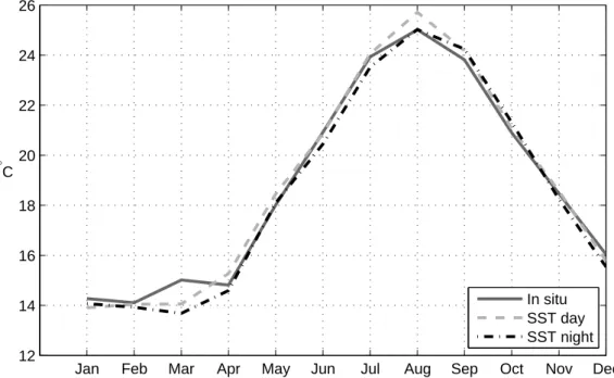
and November, during which more than 800 measurements were made per month. The number of satellite data interpolated at the in situ locations is much smaller, due principally to the presence of clouds in this data set. As a result, there are about 34% of in situ data that can be compared to day-time or night-time satellite data. The distribution through the hours of the day (figure 3) of the in situ data is homogeneous, with only a slightly higher percentage of data taken during day-time hours (54.56%) compared to night-time hours (45.44%). The comparison with satellite data will there-fore not be biased by inhomogeneous data distribution. There are specific times of the day with a very high number of data. These have been identi-fied as ship data. Presumably, a high number of ships have an automated procedure for the recording of surface temperature data, and it is possible that this procedure is more often established at precise hours four times a day. The monthly average temperature for in situ and satellite data (interpo-lated at the in situ data locations) is shown in figure 4. Both day-time and night-time satellite data reproduce closely the annual temperature cycle as described by in situ data, although day-time satellite temperatures present an anomalously high temperature in August. Both day-time and night-time satellite data sets are about 1◦C colder than in situ data in March.
Figure 5 shows the temperature distribution of the in situ and satellite data. The distribution for both types of data presents two peaks, a small one at about 14◦C and a larger one at about 20 to 25◦C. In order to assess the
effect on the heterogeneous spatio-temporal distribution of the in situ mea-surements, a histogram of the full day-time satellite SST data set is included as well (the distribution of night-time satellite SST is similar to day-time satellite SST). The full satellite data set distribution presents two peaks as well, although in this case the cold peak is much larger than the warm peak. The warm peak in the in situ data might be due to the higher number of these data being collected from September to November, which as seen on figure 4 have an average value of about 20 to 22◦C. Fewer in situ data are
collected during the winter months, which is probably the reason why the cold peak is less pronounced than the warm peak.
In order to establish the effect of the presence of clouds in the satellite data distribution, we have calculated the distribution for the cloud-free SST data obtained by applying DINEOF (Beckers and Rixen, 2003; Alvera-Azc´arate et al., 2005) to the data set used in this work. The temperature distribu-tion of a pentad AVHRR climatology (available at http://data.nodc.noaa. gov/pathfinder/CoralAtlas/PathfinderSST_Climatologies/5day/) has
been calculated as well. Both of these data sets present a distribution simi-lar to the cloudy data set in figure 5 (not shown), which gives us confidence in that it represents correctly the western Mediterranean SST distribution. Given these results, we can confirm that the different spatial and temporal distributions of in situ and satellite data are causing the differences observed in the temperature distributions of figure 5.
The in situ data distribution has been also represented separately for each season (figure 6): the contribution of winter data (season 1, January to March) and spring data (season 2, April to June) to the cold peak becomes apparent in this figure, while the warm peak in the distribution of in situ data is due, as thought, to the high number of data taken in late summer and fall. The distribution of the satellite data interpolated to the in situ positions is very similar to the distribution of in situ data for each season, in terms of position and relative size of peaks and minimum and maximum values.
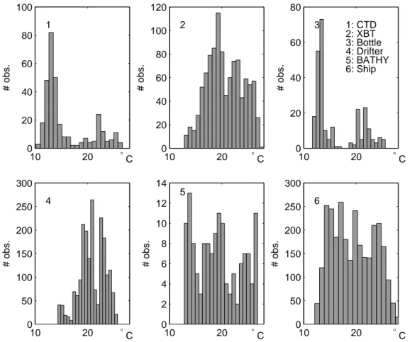
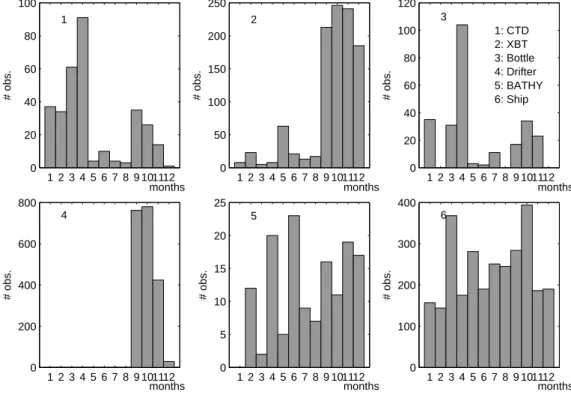
The temperature distribution for each sensor type, and their distribution in time (figures 7 and 8 respectively) add some information on the in situ data distribution: the warm peak is mainly due to drifter and XBT data, both data sets mostly taken from September to December. The cold winter peak consists mainly of ship, CTD and to a lesser extent, bottle data. Ship data distribution is quite homogeneous during the year (figure 8), therefore the histogram for this type of data (figure 7) is the most similar to the com-plete distribution of satellite data.
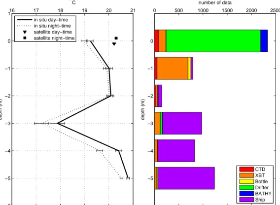
The average temperature for each depth considered (from 0 to 5 m depth) was calculated using all in situ data. In order to verify our approach of us-ing all in situ data when comparus-ing with satellite data, we divided the in situ data into day-time and night-time data, using the day-night distribution used in figure 3. The results are presented in figure 9, where the average temperature for day and night satellite data (interpolated to the in situ posi-tions) is included as well. It can be seen that, for data up to 3 m depth, the difference between in situ data and satellite data is larger that any differences induced by the time of the day at which the data are taken. This validates the approach of using all in situ data (day and night time) in our subsequent comparisons. For data at 4 and 5 m depth it is less straightforward to make this assertion. Also, it appears that in situ data at 1-2 m depth are the closest to the satellite estimate, which indicates that the satellite data are effectively representing the bulk temperature of the Mediterranean Sea for this particular data set. The temperature minimum observed at 3 m depth
is mostly caused by ship data. These ship data are taken during all months in 1999 and homogeneously through all the western Mediterranean Seaso it is unlikely that these data come from a single mis-calibrated sensor. It may be possible that there is a bias inherent to a specific ship temperature sensor mounted at 3 m depth, or induced by the architecture of a specific type of ship. The identification of the particular type of ships carrying a tempera-ture sensor at 3 m depth is however beyond the scope of this work. These data should probably be removed from the merging analysis.
4
Comparison between in situ and satellite
data
As stated previously, the ultimate objective in mind for this work, although not part of it, is to use the error assessment for an optimal merging of the satellite and in situ data. Given the small number of in situ observations compared to satellite observations, the impact of the in situ data can be very limited in the final merged product. Because of that, in this section we com-pare all available in situ data to either the night-time or day-time satellite data. The error statistics obtained in this section will determine if using all in situ data (regardless of the hour of the day at which they are taken) to be merged with either night-time or day-time satellite data is a valid approach.
4.1
Error by sensor type
Several error measures (bias, root-mean squared (RMS) error, correlation and standard deviation of the different data sets) are used to assess the dif-ferences between in situ and satellite data. The last three measures are nicely condensed into the Taylor diagram (Taylor, 2001), which is presented in fig-ure 10 for the comparison between day-time satellite data and in situ data, and in figure 11 for the comparison between night-time satellite data and in situ data. For each of these comparisons, the data have been grouped into months (subfigures 10(a) and 11(a)), and into sensor-type (subfigures 10(b) and 11(b)). In this last case, the average value for each month is previously subtracted from the data to remove the annual cycle. Note that the satellite data are normalized by the standard deviation of the in situ data. In situ data are positioned in the x-axis with a standard deviation of 1 and the error of the other data being compared is established as the linear distance to this point
(centered RMS), the angle to the x-axis (correlation) and distance to the ori-gin (standard deviation, where data with a standard deviation lower/higher than one have a standard deviation lower/higher than the reference data set). For both night and day satellite data, spring and summer months present the highest RMS errors and lowest correlations. There is no apparent differ-ence between night-time and day-time satellite data, which would be indi-cated by a higher clustering of one of them around the reference point (the in situ data). If the Taylor diagrams are repeated without the ship data (figures not shown), then it becomes clear that night-time data are closer to the in situ data than day-time satellite data. It appears that the ship data introduce a higher variability in the comparisons. When looking at the error for each type of sensor, the comparison with night-time satellite data yields the best results, with ship data the platform with the worst performance, as already mentioned above. One of the best comparisons is obtained between bottle data and night-time satellite data. In the comparison with day-time satellite data, bottle, CTD and ship data present the highest errors. Note that the bias is not included in Taylor diagrams. The fact that night-time satellite data compares better to in situ data than day-time satellite data re-inforces the practice of relating the in situ SST measurements to night-time satellite SST estimates, to avoid the problem of diurnal warming.
In order to complete the information included in figures 10 and 11, table 3 contains the bias and centered RMS error (i.e. the RMS error without the contribution of the bias) of the satellite data respect to in situ data, and the standard deviation of both satellite and in situ data, divided again by sensor type. The highest bias is found in the comparison with ship data, with night-time satellite data half a degree colder than in situ data. The comparison with drifters also yields a high bias, for both night-time and day-time satellite data, and in this case the satellite data are warmer than the drifter data. The sign of the bias cannot be explained in either case by the average depth at which these measurements are taken (table 1), because ship data are the deepest (4 m depth in average) and drifter data are one of the shallowest (0.06 m depth in average). Our results agree with other works that account for a cold bias in drifter data respect to ship data (e.g. Emery et al., 2001a; Ingleby, 2010), and a warm bias in ship data (e.g. Kent et al., 1993, 2010), more specifically in engine room intake measurements. Given that the ship data set we are using consists mostly of engine room intake measurements (78.5%), the observed warm bias must be mostly due to this effect. The centered RMS error is the highest when comparing satellite data with ship data, CTD data and BATHY data.
The error assessment mentioned above compares satellite and in situ data only at those positions were satellite data is available. In other words, when clouds are present the error between in situ and satellite data can obviously not be calculated. Any error measure concerning infrared satellite data will result in a “clear-sky” estimation. This explains the apparent contradiction between, for example, the warm bias of ship data presented in table 3 and the average temperature (colder than satellite data) of ship data in figure 9. In figure 9 all ship data are used to calculate the average value, whereas in table 3 only ship data for which there are matching satellite observations are used. Considering that the surface of the sea might be warmer under clear sky conditions (because of the increased solar radiation reaching the surface of the sea), it is therefore expected that the in situ data average is warmer when we consider only those points where there are no clouds.
The particular contribution of each sensor/platform type to the overall bias is presented as an histogram in figure 12, again divided by sensor type. A peak is found at about -4◦C caused by ship data, both for the day-time
and night-time satellite data sets. This appears to indicate an erroneous set of ship data with values much warmer than satellite data, rather than an wrongly detected cold zone in the satellite data set (for example an unde-tected cloud), which will likely appear at more than one sensor type. Further investigation on the origin of this peak in the histogram reveals that these are data taken consecutively from the 10th to the 30th March 1999 in the Gulf of Lions area, which indicates that these data may come from a single ship. The difference of about 1◦C between satellite and in situ data during March
(figure 4) is explained by the presence of these ship data. The histogram in figure 12 also shows the positive bias of satellite data respect to drifter data, and the warm bias of night-time satellite data respect to CTDs.
Visually, some of the distributions appear to be skewed. In order to test is the distributions can be described as Gaussian, an Anderson-Darling test (Anderson and Darling, 1952) has been applied. For all data types together the test concluded that, with a confidence of 99%, the difference distribution is not normal for both the day-time and night-time cases. Applying the test sensor by sensor, all sensors present a non-normal distribution at the 99% level of confidence, except BATHY for day-time data and bottles and drifters for night-time data, for which the hypothesis of non-normality cannot be re-jected. The non-normality of the data difference distributions has important consequences for several analysis techniques, as in data assimilation and the merging of the satellite and in situ data sets.
4.2
Error by database
A last test is performed to assess the quality of the in situ data organized by database. The results of this assessment are presented in figure 13 and in table 4. ICOADS data is composed solely of ship data, and the rest of the databases provided data from all the other platforms except ship data. This makes difficult the comparison between ICOADS and the rest of the databases. As already discussed in the previous sub-section, ship data from ICOADS presents the highest RMS error and biases, which is reflected in figure 13 and table 4. ICES data follow in the Taylor diagram. There is lit-tle difference in the quality of each database when comparing with day-time or night-time satellite data. Apart from ICOADS, the databases WOD and Coriolis present the highest bias (table 4), with satellite colder than in situ data for WOD and warmer than in situ data for Coriolis. In general, all pre-sented databases have very similar correlation with satellite data, although when the annual cycle is removed, ICOADS data and ICES data perform poorly in terms of correlation.
5
Conclusions
A comparison between in situ and satellite sea surface temperature (SST) has been realised in the western Mediterranean Sea for 1999. Five interna-tional databases have been used to extract in situ data for the desired period and zone: World Ocean Database (WOD), MEDAR/Medatlas, Coriolis, In-ternational Council for the Exploration of the Sea (ICES) and InIn-ternational Comprehensive Ocean-Atmosphere Data Set (ICOADS). The in situ data have been classified into different platforms or sensors, in order to compare the relative accuracy of these type of data respect to the satellite data. The statistics obtained during this study will be used in future work for merging purposes.
Ship data, from the ICOADS database, are the most numerous, and as such they are a valuable source of data. However, the error assessment be-tween these data and satellite data shows a large bias and RMS error. A series of suspect data were identified with a large bias (more than 3◦C warmer than
satellite data) and that presumably came from a single ship as they were lo-calized in time and space. One must bear in mind that the ships collecting
surface temperature data are very heterogeneous in size, and therefore the resulting measurements are very heterogeneous as well. In addition, mea-surements from ships (and other platforms in general) are not made with the purpose of complementing satellite data, therefore they do not necessarily represent the same temperature.
Other types of data performed more homogeneously, with RMS errors of 0.6 to 0.9◦C and small biases. The largest bias was detected for drifter data,
which was in average 0.48◦C and 0.42◦C colder than day-time and night-time
satellite data respectively. This cold bias in drifter data is maybe unexpected given that the drifters average depth was of 0.06 m, one of the shallowest among the platforms considered in this work. The fact that satellite data are calibrated using in situ buoys measuring bulk temperatures can be the reason for this bias. If a given sensor is directly exposed to the air, for example dur-ing calm sea conditions, this might induce as well a cold bias in the drifters measurements. The fact that most of the drifters were released during fall 1999, a period during which there can have been a cooling of the air in the Gulf of Lions region, reinforces this possibility. If the exposure to the air is responsible for the cold bias during fall, then the opposite should be verified too, ı.e. that drifters deployed during summer and under calm sea conditions will present a warm bias. This cannot be verified in this work, as there were no drifter data deployed during summer. The smallest bias between satellite data and in situ data was observed at 1-2 m depth, which confirms that the satellite are representing the bulk temperature of the Mediterranean Sea, at least for this particular data set.
The satellite-in situ SST difference distribution is generally not normal, as showed by an Anderson-Darling test at the 99% level of confidence. This result is obtained when using all in situ data types and for individual sensor types. Only the difference distribution between satellite and BATHY, bot-tle and drifter data cannot be considered non-normal using the mentioned test. The non-normality of the data difference distributions has important consequences for several analysis techniques, as in data assimilation and the merging of the satellite and in situ data sets. This factor needs therefore to be taken into account in future work.
Apart from the error assessment by data type, the average error for each database was as well calculated. ICOADS, containing only ship data, presents the highest errors. The rest of the databases have similar RMS er-rors among them, but in terms of bias, WOD and ICES presented the highest deviations respect to satellite data.
The comparison of satellite infrared data with in situ data is limited by the presence of clouds in the atmosphere, which prevents the infrared radia-tion from the sea surface to reach the satellite. The error measures presented in this work reflect therefore clear-sky conditions. The presence or absence of clouds influences the sea surface temperature. In the absence of clouds, the solar radiation reaching the surface of the sea during the day increases. The absence of clouds affects also the net long-wave radiation budget at the ocean surface (the amount of long-wave radiation reflected back to the ocean is reduced). This may specially affect the bias between in situ and satellite data, as well as other error measures.
The results obtained in this work emphasize that the differences between in situ and satellite SST data can be affected by various factors (database, sensor or platform type, specific bias at a particular platform, etc). A careful study of these differences is needed prior to any work aiming to use these sources of data in a joint manner.
Acknowledgements
This work was realised in the context of the HiSea - SR/12/140 project funded by the Belgian Science Policy (BELSPO) in the frame of the Research Pro-gram For Earth Observation “STEREO II”. The AVHRR Oceans Pathfinder SST data were obtained through the online PO.DAAC Ocean ESIP Tool (POET) at the Physical Oceanography Distributed Active Archive Center (PO.DAAC), NASA Jet Propulsion Laboratory, Pasadena, CA. The different providers for the databases used (World Ocean Database, MEDAR/MedAtlas, Coriolis Data Center, the International Council for the Exploration of the Sea and the International Comprehensive Ocean-Atmosphere Data Set) are also acknowledged for their important work of compiling extensive amounts of data and making them publicly available. The National Fund for Scientific Research, Belgium, is acknowledged for funding the post-doctoral positions of A. Alvera-Azc´arate and A. Barth and for funding C. Troupin’s thesis through a FRIA grant. This is a MARE publication.
References
Alvera-Azc´arate, A., Barth, A., Rixen, M., Beckers, J.-M., 2005. Reconstruc-tion of incomplete oceanographic data sets using Empirical Orthogonal Functions. Application to the Adriatic Sea surface temperature. Ocean Modelling. 9, 325–346, doi:10.1016/j.ocemod.2004.08.001.
Alvera-Azc´arate, A., Sirjacobs, D., Barth, A., Beckers, J.-M., 2010. Out-lier detection in satellite data using spatial coherence. Remote Sensing of Environment. Submitted.
Anderson, T. W., Darling, D. A., 1952. Asymptotic theory of certain ”goodness-of-fit” criteria based on stochastic processes. Annals of Mathe-matical Statistics 23, 193–212.
Barton, I., 2007. Comparison of In Situ and Satellite-Derived Sea Surface Temperatures in the Gulf of Carpentaria. Journal of Atmospheric and Oceanic Technology 24, 1773–1784.
Beckers, J.-M., Rixen, M., 2003. EOF calculations and data filling from in-complete oceanographic data sets. Journal of Atmospheric and Oceanic Technology 20 (12), 1839–1856.
Castro, S. L., Wick, G. A., Jackson, D. L., Emery, W. J., 2008. Error characterization of infrared and microwave satellite sea surface temper-ature products for merging and analysis. Journal of Geophysical Research 113 (C03010), doi:10.1029/2006JC003829.
Donlon, C., Casey, K. S., Robinson, I. S., Gentemann, C. L., Reynolds, R. W., Barton, I., Arino, O., Stark, J., Rayner, N., Le Borgne, P., Poulter, D., Vazquez-Cuervo, J., Armstrong, E., Beggs, H., Llewellyn-Jones, D., Minnett, P. J., Merchant, C. J., Evans, R., 2009. The GODAE High-Resolution Sea Surface Temperature Pilot Project. Oceanography 22 (3), 34–45.
Emery, W., Baldwin, D. J., Schl¨ussel, P., Reynolds, R., 2001a. Accuracy of in situ sea surface temperatures used to calibrate infrared satellite mea-surements. Journal of Geophysical Research 106 (C2), 2387–2405.
Emery, W., Castro, S., Wick, G., Schluessel, P., Donlon, C., 2001b. Esti-mating Sea Surface Temperature from Infrared Satellite and In Situ Tem-perature Data. Bulletin of the American Meteorological Society 82 (12), 2773–2785.
Gentemann, C., Minnett, P., Sienkiewicz, J., DeMaria, M., Cummings, J., Jin, Y., Doyle, J., Gramer, L., Barron, C., Casey, K., Donlon, C., 2009. MISST: The Multi-Sensor Improved Sea Surface Temperature Project. Journal of Oceanography 22 (2), 78–89.
Guan, L., Kawamura, H., 2004. Merging Satellite Infrared and Microwave SSTs: Methodology and Evaluation of the New SST. Journal of Oceanog-raphy 60, 905–912.
Ingleby, B., 2010. Factors Affecting Ship and Buoy Data Quality: A Data Assimilation Perspective. Journal of Atmospheric and Oceanic Technology 27, 1476–1489.
Kent, C., Kennedy, J., Berry, D., Smith, R., 2010. Effects of instrumenta-tion changes on sea surface temperature measured in situ. WIREs Climate Change 1 (5), 718–728, doi:10.1002/wcc.55.
Kent, C., Taylor, P., Truscott, B., Hopkins, J., 1993. The accuracy of Volun-tary Observing Ships’ Meteorological Observations - Results of the VSOP-NA. Journal of Atmospheric and Oceanic Technology 10, 591–608.
Kent, E., Challenor, P., 2006. Toward Estimating Climatic Trends in SST. Part II: Random Errors. Journal of Atmospheric and Oceanic Technology 23, 476–486.
Locarnini, R. A., Mishonov, A. V., Antonov, J. I., Boyer, T. P., Garcia, H. E., 2006. World Ocean Atlas 2005, Volume 1: Temperature. Tech. rep., NOAA, Washington D.C., 182pp.
MEDAR-Group, 2002. MEDATLAS/2002 database. Mediterranean and Black Sea database of temperature salinity and bio-chemical parameters. Climatological Atlas. Ifremer edition 4 CD-ROM.
Reynolds, R., Smith, T., Liu, C., Chelton, D., Casey, K., Schlax, M., 2007. Daily high-resolution-blended analyses for sea surface temperature. Jour-nal of Climate 20, 5473–5496.
Robinson, I. S., 2004. Measuring the oceans from space. The principles and methods of satellite oceanography. Springer-Praxis, 669 pp.
Sirjacobs, D., Alvera-Azc´arate, A., Barth, A., Lacroix, G., Park, Y., Nechad, B., Ruddick, K., Beckers., J.-M., 2010. Cloud filling of ocean color and sea surface temperature remote sensing products over the southern north sea by the data interpolating empirical orthogonal functions methodology. Journal of Sea ResearchAccepted.
Taylor, K. E., 2001. Summarizing multiple aspects of model performance in a single diagram. Journal of Geophysical Research 106, D7, 7183–7192. Xu, F., Ignatov, A., 2010. Evaluation of in situ sea surface temperatures
for use in the calibration and validation of satellite retrievals. Journal of Geophysical Research 115, C09022, doi:10.1029/2010JC006129.
Table 1: Number of observations available for this work, average depth for each of them, and coincident satellite observations.
In situ Depth (m) Satellite (day-time) Satellite (night-time)
CTD 320 0.86 124 95 XBT 1043 1.41 287 325 Bottle 260 1.96 73 64 Float/Drifter 1994 0.06 737 729 Bathy 141 0.02 46 60 Tesac 13 0 5 0 Ship 2865 4 969 1008 Total 6636 2241 2281
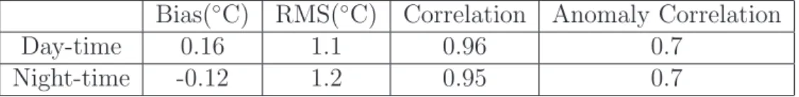
Table 2: Errors between in situ data and AVHRR satellite data. Day-time and night-time refer to satellite time passage, but all in situ data are compared with each of these data sets.
Bias(◦C) RMS(◦C) Correlation Anomaly Correlation
Day-time 0.16 1.1 0.96 0.7
Night-time -0.12 1.2 0.95 0.7
Table 3: Errors between in situ data and AVHRR satellite data, for each sensor type. Day-time and night-time refer to satellite time passage, but all in situ data are compared with each of these data sets.
Bias(◦C) Centered RMS(◦C) σ satellite (◦C) σ in situ(◦C)
CTD Day-time 0.42 0.75 4.33 4.33 Night-time -0.1 0.61 4.6 XBT Day-time -0.0 0.69 3.43 3.37 Night-time -0.15 0.66 3.63 Bottle Day-time 0.27 0.82 4.47 4.18 Night-time -0.05 0.51 4.54 Drifter Day-time 0.48 0.52 2.19 2.43 Night-time 0.42 0.68 2.47 Bathy Day-time -0.18 0.68 4.0 4.25 Night-time -0.33 0.89 3.85 Tesac Day-time -0.27 0.12 0.13 0.47 Night-time – – – Ship Day-time -0.1 1.4 4.5 4 Night-time -0.5 1.5 4.4
Table 4: Errors between in situ data and AVHRR satellite data, for each data base. Day-time and night-time refer to satellite time passage, but all in situ data are compared with each of these data sets.
Bias(◦C) Centered RMS (◦C) Correlation Anomaly corr.
ICOADS Day-time 0.05 1.43 0.95 0.53 Night-time 0.5 1.5 0.94 0.51 ICES Day-time -0.36 0.72 0.99 0.64 Night-time 0 0.48 0.99 0.56 Coriolis Day-time 0.11 0.64 0.98 0.86 Night-time 0.24 0.66 0.98 0.81 Medatlas Day-time -0.01 0.68 0.98 0.81 Night-time 0.15 0.56 0.99 0.74 WOD Day-time -0.39 0.62 0.98 0.84 Night-time -0.25 0.73 0.97 0.82 4oW 0o 4oE 8oE 12oE 36oN 38oN 40oN 42oN 44oN ship CTD XBT Bottle Drifter BATHY TESAC
Figure 1: Spatial distribution of the in situ data divided by sensor/platform type.
Jan Feb Mar Apr May Jun Jul Aug Sep Oct Nov Dec 0 200 400 600 800 1000 1200 1400 1600 # obs in situ Satellite day Satellite night
Figure 2: Number of in situ observations, satellite day-time data and satellite night-time data for each month of the year 1999.
0 5 10 15 20 25 0 100 200 300 400 500 600 700 hours number of observations Night, 45.44% Day, 54.56%
Figure 3: Number of in situ observations for each hour of the day.
Jan Feb Mar Apr May Jun Jul Aug Sep Oct Nov Dec 12 14 16 18 20 22 24 26 °C In situ SST day SST night
Figure 4: Monthly average temperature for in situ, day-time and night-time satellite data.
10 20 30 0 200 400 600 800 ° C # obs. a 10 20 30 0 100 200 300 ° C # obs. c 10 20 30 0 1 2 x 10⁶ ° C # obs. b 10 20 30 0 100 200 300 ° C # obs. d
Figure 5: Temperature distribution in 1999 of (a) all in situ data; (b) all day-time satellite data; (c) day-time satellite data interpolated at the in situ positions; and (d) night-time satellite data interpolated at the in situ positions. Note that the vertical scales are different in each subplot.
10 15 20 25 0 100 200 300 400 01 # obs. 10 15 20 25 0 100 200 300 400 03 # obs. 10 15 20 25 0 100 200 300 400 02 # obs. 10 15 20 25 0 100 200 300 400 04 # obs. ° C ° C ° C ° C
Figure 6: Temperature distribution of in situ data for each season (1: January-March; 2: April-June; 3: July-September; 4: October-December).
10 20 0 20 40 60 80 100 # obs. 1 10 20 0 50 100 150 200 250 300 # obs. 4 10 20 0 20 40 60 80 100 120 # obs. 2 10 20 0 2 4 6 8 10 12 14 # obs. 5 10 20 0 20 40 60 80 # obs. 3 1: CTD 2: XBT 3: Bottle 4: Drifter 5: BATHY 6: Ship ° C ° C ° C 10 20 0 50 100 150 200 250 300 # obs. 6 ° C ° C ° C
Figure 7: Temperature distribution of in situ data for each sensor. The x-axis denotes the temperature in ◦C, and the y-axis indicates number of
1 2 3 4 5 6 7 8 9 101112 0 20 40 60 80 100 # obs. 1 1 2 3 4 5 6 7 8 9 101112 0 200 400 600 800 # obs. 4 1 2 3 4 5 6 7 8 9 101112 0 50 100 150 200 250 # obs. 2 1 2 3 4 5 6 7 8 9 101112 0 5 10 15 20 25 # obs. 5 1 2 3 4 5 6 7 8 9 101112 0 20 40 60 80 100 120 # obs. 3 1: CTD 2: XBT 3: Bottle 4: Drifter 5: BATHY 6: Ship months months months 1 2 3 4 5 6 7 8 9 101112 0 100 200 300 400 # obs. 6 months months months
Figure 8: Temporal distribution of in situ data. The x-axis denotes the months of the year, and the y-axis indicates number of observations. Note the different scales in the vertical axes.
16 17 18 19 20 21 −6 −5 −4 −3 −2 −1 0 1 ° C depth (m) 0 500 1000 1500 2000 2500 −5 −4 −3 −2 −1 0 number of data depth (m) in situ day−time in situ night−time satellite day−time satellite night−time CTD XBT Bottle Drifter BATHY Ship
Figure 9: Left panel: average temperature with depth for the in situ data, divided in night-time and day-time data. The horizontal bars represent the standard error of the mean. The average temperature for day and night satellite data (interpolated to the in situ positions) is also included. Note that the depth of the night and day satellite data is different from 0m only to improve their readability. Right panel: number of data for each sensor category at each depth.
Figure 10: Taylor diagram of the comparison between day-time satellite with in situ data for (a) each month and (b) each sensor. Gray isolines represent
Figure 11: Taylor diagram of the comparison between night-time satellite with in situ data for (a) each month and (b) each sensor. Gray isolines
Figure 12: Histogram of the difference between satellite data and in situ data, for (a) day-time satellite data and (b) night-time satellite data. Negative (positive) values represent a cold (warm) bias in the satellite data respect to in situ data.
Figure 13: Taylor diagram presenting the error between in situ data organized by database and satellite data (used as reference). Top panel: day-time satellite data are used. Bottom panel: night-time satellite data are used. The annual cycle has been subtracted before the calculation of the errors.