A search for transiting planets around hot subdwarfs: I. Methods and performance tests on light curves from Kepler, K2, TESS, and CHEOPS

May 5, 2021

A search for transiting planets around hot subdwarfs: I. Methods

and performance tests on light curves from Kepler, K2, TESS,

and CHEOPS

‹

V. Van Grootel

, F. J. Pozuelos

, A. Thuillier

, S. Charpinet

, L. Delrez

, M. Beck

, A. Fortier

, S.

Hoyer

, S. G. Sousa

, B. N. Barlow

, N. Billot

, M. Dévora-Pajares

, R. H. Østensen

, Y. Alibert

, R.

Alonso

, G. Anglada Escudé

, J. Asquier

, D. Barrado

, S. C. C. Barros

, W. Baumjohann

, T.

Beck

, A. Bekkelien

, W. Benz

, X. Bonfils

, A. Brandeker

, C. Broeg

, G. Bruno

, T. Bárczy

, J.

Cabrera

_{, A. C. Cameron}

_{, S. Charnoz}

_{, M. B. Davies}

_{, M. Deleuil}

_{, O. D. S. Demangeon}

_{, B.-O.}

Demory

, D. Ehrenreich

, A. Erikson

, L. Fossati

, M. Fridlund

, D. Futyan

, D. Gandolfi

, M.

Gillon

, M. Guedel

, K. Heng

, K. G. Isaak

, L. Kiss

, J. Laskar

, A. Lecavelier des Etangs

, M.

Lendl

, C. Lovis

, D. Magrin

, P. F. L. Maxted

, M. Mecina

, A. J. Mustill

, V. Nascimbeni

, G.

Olofsson

, R. Ottensamer

, I. Pagano

, E. Pallé

, G. Peter

, G. Piotto

, J.-Y. Plesseria

, D.

Pollacco

, D. Queloz

, R. Ragazzoni

, N. Rando

, H. Rauer

, I. Ribas

, N. C. Santos

, G.

Scandariato

, D. Ségransan

, R. Silvotti

, A. E. Simon

, A. M. S. Smith

, M. Steller

, G. M. Szabó

,

N. Thomas

, S. Udry

, V. Viotto

, N. A. Walton

, K. Westerdorff

, and T. G. Wilson

(Affiliations can be found after the references)

Received ...; Accepted... ABSTRACT

Context. Hot subdwarfs experienced strong mass loss on the red giant branch (RGB) and are now hot and small He-burning objects.

These stars constitute excellent opportunities for addressing the question of the evolution of exoplanetary systems directly after the RGB phase of evolution.

Aims. In this project we aim to perform a transit survey in all available light curves of hot subdwarfs from space-based telescopes

(Kepler, K2, TESS, and CHEOPS) with our custom-made pipeline SHERLOCK in order to determine the occurrence rate of planets around these stars as a function of orbital period and planetary radius. We also aim to determine whether planets that were previously engulfed in the envelope of their red giant host star can survive, even partially, as a planetary remnant.

Methods. For this first paper, we performed injection-and-recovery tests of synthetic transits for a selection of representative Kepler,

K2, and TESS light curves to determine which transiting bodies in terms of object radius and orbital period we will be able to detect with our tools. We also provide estimates for CHEOPS data, which we analyzed with the pycheops package.

Results. Transiting objects with a radius À 1.0 RC can be detected in most of the Kepler, K2, and CHEOPS targets for the

shortest orbital periods (1 d and shorter), reaching values as low as „0.3 RC in the best cases. Sub-Earth-sized bodies are only

reached for the brightest TESS targets and for those that were observed in a significant number of sectors. We also give a series of representative results for larger planets at greater distances, which strongly depend on the target magnitude and on the length and quality of the data.

Conclusions. The TESS sample will provide the most important statistics for the global aim of measuring the planet occurrence

rate around hot subdwarfs. The Kepler, K2, and CHEOPS data will allow us to search for planetary remnants, that is, very close and small (possibly disintegrating) objects.

Key words. planet-star interactions; planetary systems; stars: RGB; stars: horizontal branch; stars: subdwarfs; techniques: photo-metric

1. Introduction

Hot subdwarf B (sdB) stars are hot and compact stars (Teff “ 20 000 ´ 40 000 K and log g “ 5.2 to 6.2;

Saf-fer et al. 1994) that lie on the blue tail of the horizon-tal branch (HB), that is, the extreme horizonhorizon-tal branch (EHB). The HB stage corresponds to core-He burning

ob-Send offprint requests to: V. Van Grootel

‹ _{CHEOPS data presented in Fig. 5 and lists presented in}

AppendixCandDare available in electronic form at the CDS

via anonymous ftp to cdsarc.u-strasbg.fr (130.79.128.5) or

viahttp://cdsweb.u-strasbg.fr/cgi-bin/qcat?J/A+A/

jects and follows the red giant branch (RGB) phase. Unlike most post-RGB stars that cluster at the red end of the HB (the so-called red clump, RC) because they lose almost no envelope on the RGB (Miglio et al. 2012), sdB stars expe-rienced strong mass loss on the RGB and have extremely thin residual H envelopes (Menv ă 0.01Md, Heber 1986).

This extremely thin envelope explains their high effective temperatures and their inability to sustain H-shell burn-ing. This prevents these stars from ascending the asymp-totic giant branch (AGB) after core-He exhaustion ( Dor-man et al. 1993). About 60% of the sdBs reside in binary

systems, and about half of them are in close binaries with orbital periods of up to a few days (see, e.g., Allard et al. 1994; Maxted et al. 2001), while the other half resides in wider binaries with orbital periods of up to several years (Stark & Wade 2003; Vos et al. 2018). Binary interactions (through common-envelope, CE, evolution for the short or-bits, and stable Roche-lobe overflow, RLOF, evolution for the wide orbits) are therefore the main reasons for this ex-treme mass loss (Han et al. 2002, 2003). The hot O-type subdwarfs, or sdO stars, have Teff “ 40 000 ´ 80 000 K and

a wide range of surface gravities. The compact sdO stars (log g “ 5.2 ´ 6.2) are either post-EHB objects or direct post-RGB objects (through a so-called late hot He-flash;

Miller Bertolami et al. 2008), or end products of merger events (Iben 1990; Saio & Jeffery 2000, 2002). The sdOs with log g < 5.2 are post-AGB stars, that is, stars that have ascended the giant branch a second time after core-He burning exhaustion (Reindl et al. 2016).

The formation of the approximately 40% of sdB stars that appear to be single has been a mystery for decades. In the absence of a companion, it is hard to explain how the star can expel most of its envelope on the RGB and still achieve core-He burning ignition. Recently, Pelisoli et al.

(2020) suggested that all sdB stars might originate from binary evolution. Merger scenarios involving two low-mass white dwarfs have also been investigated (Webbink 1984;

Han et al. 2002, 2003; Zhang & Jeffery 2012), but sev-eral facts challenge this hypothesis. First, compact low-mass white dwarf binaries are quite rare, even though some candidates are identified (Ratzloff et al. 2019). Second, the mass distributions of single and binary sdB stars are indis-tinguishable (Fontaine et al. 2012, Table 3 in particular). This mass distribution is mainly obtained from asteroseis-mology (some sdB stars exhibit oscillations, which allow the precise and accurate determination of the stellar parame-ters, including total mass; Van Grootel et al. 2013) and also from binary light-curve modeling for hot subdwarfs in eclipsing binary systems. Single and binary mass distribu-tions peak at „ 0.47Md, which is the minimum core mass

required to ignite He through a He-flash at the tip of RGB (stars of Á 2.3Md are able to ignite He quietly at lower

core masses, down to „ 0.33Md, but the more massive the

stars, the rarer they are). A mass distribution of single sdB stars from mergers, in contrast, would be much broader (0.4´0.7 Md; Han et al. 2002). With the DR2 release of

Gaia (Gaia Collaboration et al. 2018) and precise distances for many hot subdwarfs (Geier 2020), it is now also possi-ble to build a spectrophotometric mass distribution for a much larger sample than what was achieved with the hot subdwarf pulsators or those in eclipsing binaries. Individ-ual masses are much less precise than those obtained by asteroseismology or binary light-curve modeling (Schneider et al. 2019). However, single and binary spectrophotometric mass distributions share the same properties here as well, which tends to disprove the hypothesis of different origins for single and binary sdB stars. The third piece of evidence against merger scenarios (which would most likely result in fast-rotating objects) is the very slow rotation of almost all single sdB stars, as obtained through v sin i measurements (Geier & Heber 2012) or from asteroseismology (Charpinet et al. 2018). Moreover, their rotation rates are in direct line with the core rotation rates observed in RC stars (Mosser et al. 2012), which is another strong indication that these

stars and the single sdB stars do share a same origin, that is, that they are post-RGB stars.

The question of the evolution of exoplanet systems after the main sequence of their host is generally addressed by studying exoplanets around subgiants, RGB stars, and nor-mal HB (RC) stars (hereafter the ’classical’ evolved stars). These classical evolved stars are typically very large stars, with radii ranging from „ 5´10 Rdto more than 1000 Rd.

This is much larger than hot subdwarfs, which have radii in the range „ 0.1 ´ 0.3 Rd (Heber 2016). Their mass is

typically higher than „ 1.5 Md, compared to „ 0.47Mdfor

hot subdwarfs. The transit and radial velocity (RV) meth-ods are both challenging for these classical evolved stars because the transit depth is diluted and there are addi-tional noise sources (Van Eylen et al. 2016). Another dif-ficulty for the question of the fate of exoplanet systems after the RGB phase itself is the difficulty of distinguishing RGB and RC stars based on their spectroscopic parameters alone, which is sometimes hard even with help of astero-seismology (Campante et al. 2019). As a consequence, only large or massive planets are detected around the classical evolved stars (Jones et al. 2020, and references therein). A dearth of close-in giant planets is observed around these evolved stars compared to solar-type main-sequence stars (Sato et al. 2008;Döllinger et al. 2009). This may be caused by planet engulfment by the host star, but current technolo-gies do not allow us to determine whether smaller planets and remnants (such as the dense cores of former giant plan-ets) are present. The lack of close-in giant planets may also be explained by the intrinsically different planetary forma-tion for these intermediate-mass stars (see the discussion in

Jones et al. 2020). Ultimately, the very existence of planet remnants may be linked to the ejection of most of the en-velope on the RGB that occurs for hot subdwarfs, while for classical evolved stars, nothing stops the in-spiraling planet inside the host star, and in all cases, the planet fi-nally merges with the star, is fully tidally disrupted, or is totally ablated by heating or by the strong stellar wind. In other words, the ejection of the envelope not only enables the detection of small objects as remnants, but most impor-tantly, it may even be the reason for the existence of these remnants by stopping the spiraling-in in the host star.

Many studies have focused on white dwarfs (the ulti-mate fate of „97% of all stars), including the direct obser-vations of transiting disintegrating planetesimals ( Vander-burg et al. 2015), the accretion of a giant planet (Gänsicke et al. 2019), and, most recently, the transit of a giant planet (Vanderburg et al. 2020). More than 25% of all single white dwarfs exhibit metal pollution in their atmospheres (which should be pure H or He because of the gravitational set-tling of heavier elements in these objects with very high surface gravities), which is generally interpreted as mate-rial accretion of surrounding planetary remnants (Hollands et al. 2018, and references therein). Statistics on the oc-currence rate of planets around white dwarfs as a function of orbital period and planet radius have also been estab-lished (Fulton et al. 2014; van Sluijs & Van Eylen 2018;

Wilson et al. 2019). However, the vast majority of white dwarfs experienced two giant phases of evolution, namely the RGB and the AGB. The AGB expansion and strong mass loss, followed by the planetary-nebula phase, will have a profound effect on the orbital stability of the surrounding bodies (e.g.,Debes & Sigurdsson 2002;Mustill et al. 2014;

con-cerning the effect of RGB expansion alone on the exoplanet systems can be drawn from white dwarfs.

Hot subdwarfs therefore constitute excellent opportuni-ties for addressing the question of the evolution of exoplanet systems after the RGB phase of evolution. It is precisely this potential we aim to exploit in this project by determining the occurrence rate of planets around hot subdwarfs as a function of orbital period and planet radius. We achieve this objective by performing a transit search in all available light curves of hot subdwarfs from space-based observato-ries, such as Kepler (Borucki et al. 2010), K2 (Howell et al. 2014), TESS (Ricker et al. 2014), and CHEOPS (Benz et al. 2020). In this first paper, we provide a review of the current status of the search of planets around hot subdwarfs with the different detection methods in Sect. 2. We present the observations and the tools we used to perform our transit search in Sect. 3. We provide extensive tests of the photo-metric quality of the light curves in Sects.4 and5, and we conclude and outline future work in Sect. 6.

2. Search for planets around hot subdwarfs:

Current status

To date, several planet detections around hot subdwarfs have been claimed, but none of them received confirmation. With the pulsation-timing method (variation in the oscil-lation periods of sdB pulsators), planets of a few Jupiter masses in orbits at about 1 AU were announced around V391 Peg and DW Lyn (Silvotti et al. 2007; Lutz et al. 2012), but these claims have recently been refuted (Silvotti et al. 2018;Mackebrandt et al. 2020). Based on weak signals that were interpreted as reflection and thermal re-emission in Kepler light curves, five very close-in (with orbital peri-ods of a few hours) Earth-sized planets have been claimed to orbit KIC 05807616 (Charpinet et al. 2011) and KIC 10001893 (Silvotti et al. 2014). However, the attribution of these signals to exoplanets is debatable (Krzesinski 2015;

Blokesz et al. 2019). Using the RV method, Geier et al.

(2009) announced the discovery of a close-in (Porb “ 2.4

days) planet of several Jupiter masses around HD 149382, but this was ruled out by high-precision RV measurements obtained with the Hobby-Eberly Telescope spectrograph, which excluded the presence of almost any substellar com-panion with Porb ă 28 days and M sin i Á 1MJup (Norris

et al. 2011). No close massive planets (down to a few Jupiter masses) were found from a mini RV survey carried out with the HARPS-N spectrograph on eight apparently single hot subdwarfs (Silvotti et al. 2020).

Several ground-based surveys with both photometric and RV techniques target the red dwarf or brown dwarf close companions to hot subdwarfs (Schaffenroth et al. 2018, 2019). These companions are frequent (Schaffenroth et al. 2018), but no Jupiter-like planets have been found to date. In contrast, several discoveries of circumbinary mas-sive planets have been announced in close, post-CE evolu-tion sdB+dM eclipsing systems through eclipse-timing vari-ations, for instance, HW Vir, the prototype of the class (Lee et al. 2009;Beuermann et al. 2012), NSVS 14256825 (Zhu et al. 2019), HS 0705+6700 (Pulley et al. 2015), NY Vir (Qian et al. 2012), and 2M 1938+4603 (Baran et al. 2015). These planets might correspond to first-generation, second-generation (Schleicher & Dreizler 2014; Völschow et al. 2014), or hybrid planets (which are formed from ejected

stellar material that is accreted onto remnants of first-generation planets; Zorotovic & Schreiber 2013). All but one of the ten well-studied HW Vir systems show eclipse-timing variations (Heber 2016;Marsh 2018). This may call for another explanation than planets (perhaps something analogously to the mechanism suggested for eclipse-timing variations in white dwarf binaries; Bours et al. 2016) be-cause the occurrence of circumbinary planets around close main-sequence binaries that are the progenitors of such sys-tems is only „1% (Welsh et al. 2012). The properties of the claimed planets often change or are discarded after new measurements (Heber 2016;Marsh 2018), while the orbits are regularly found to be dynamically unstable (e.g., Wit-tenmyer et al. 2013). None of these claimed circumbinary planets has been confirmed through another technique.

3. Observations and methods

3.1. Space-based light curves of hot subdwarfs

In the original Kepler field, 72 hot subdwarfs were observed at the short cadence (SC) of 1 minute for at least one quar-ter, including the commissioning quarter Q0, which started on 2 May 2009. During the one-year survey phase that fol-lowed Q0 (quarters Q1 of 33.5 days and Q2 to Q4 of 90 days each, divided into monthly subquarters), 15 sdB stars were found to pulsate (Østensen et al. 2010, 2011). These 15 stars were consequently observed for the rest of the mis-sion at SC (with exceptions of some quarters for some sdB pulsators, see the details in Table A.1). Three other sdB pulsators, known as B3, B4, and B5, were found in the open cluster NGC 6791 (Pablo et al. 2011) and were ob-served at SC for various durations (see TableA.1). Of the non-pulsators, 47 B-type hot subdwarfs (sdB and sdOB) were observed for at least one month at SC (5 of them for several quarters), as well as 7 sdO stars. At the long cadence (LC) of 30 minutes, these 54 non-pulsating hot subdwarfs were generally observed for several quarters, and some of them for the whole duration of the mission. The list of hot subdwarf targets in the original Kepler field and details on the observing quarters in SC and LC can be found in Table

A.1. The primary Kepler mission stopped on 11 May 2013, during Q17.2, after the failure of a second reaction wheel that was necessary to stabilize the spacecraft and obtain the fine and stable pointing for observations of the original field.

The Kepler mission was then redesigned as K2, for which the two remaining reaction wheels allowed a stable pointing for „80 days of fields close to the ecliptic. An engi-neering test of 11 days in February 2014 confirmed the feasi-bility of this strategy, and 19 campaigns (campaign 0 to 18) were executed from March 2014 to July 2018, when exhaus-tion of propellants definitively ended the mission. When we account only for confirmed hot subdwarfs, 39 sdB/sdOB pulsators were observed at SC through at least one cam-paign in K2 fields. Two more sdB pulsators were discovered through LC data only. Seventy-nine more sdB/sdOB non-pulsators and 10 sdO non-non-pulsators were also observed at SC. Finally, 44 hot subdwarfs were observed at LC only. In contrast to Kepler, the K2 SC and LC data generally cover only one campaign (of about 80 days duration), although a few stars were observed in two or three campaigns. The full list of hot subdwarfs observed by K2 and details can be found in TableB.1.

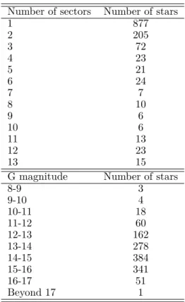
Table 1. Statistics for the hot subdwarfs observed in the pri-mary TESS mission (July 2018-July 2020).

Number of sectors Number of stars

1 877 2 205 3 72 4 23 5 21 6 24 7 7 8 10 9 6 10 6 11 13 12 23 13 15

G magnitude Number of stars

8-9 3 9-10 4 10-11 18 11-12 60 12-13 162 13-14 278 14-15 384 15-16 341 16-17 51 Beyond 17 1

TESS (Transiting Exoplanet Survey Satellite) has been operational since July 2018. It is performing a high-precision photometric survey over almost the whole sky (about 90%), avoiding only a narrow band around the eclip-tic1. The TESS primary two-year mission, which ended in early July 2020, consisted of 26 sectors that were observed nearly continuously for „27.4 days each. Some overlap be-tween sectors exists for the highest northern and south-ern ecliptic latitudes, therefore some stars have been ob-served for several sectors (see Table 1). The primary mis-sion TESS data products consist of SC observations sam-pled every 2 minutes for selected stars, as well as full-frame images (FFI) taken every 30 minutes that contain data for all stars in the field of view. Accounting for confirmed hot subdwarfs alone, 1302 stars were observed for at least one sector at SC during primary mission. This list was assem-bled by Working Group (WG) 8 on compact pulsators of the TESS Asteroseismic Consortium (TASC; see also Stassun et al. 2019). Table1presents the statistics for these TESS primary mission observations of hot subdwarfs, and the full list can be found at https://github.com/franpoz/ Hot-Subdwarfs-Catalogues(see AppendixCfor details). The TESS extended mission started on 4 July 2020, and revisits all sectors for the same duration. The sectors are referred to with increasing numbers (Sector 27, 28, etc.). An ’ultra short cadence’ of 20 s is now available in ad-dition to the normal SC of 2 minutes, and FFIs are now taken every 10 minutes. After release of Sectors 27 to 31, 243 confirmed hot subdwarfs have been observed at 20 s cadence, and 670 more at a 2-minute cadence (these tar-gets were also selected by WG8 of the TASC). Most of

1

https://tess.mit.edu/observations/

these targets were previously observed in the primary mis-sion (sectors 1 to 26), but about one-third are new tar-gets that were not observed during the primary mission. The list can be found at https://github.com/franpoz/ Hot-Subdwarfs-Catalogues(see AppendixDfor details). It is expected that about 2300 hot subdwarfs will have been observed at the end of the two-year extended mission.

CHEOPS (CHaracterising ExOPlanets Satellite) is a European Space Agency (ESA) mission primarily dedicated to the study of known extrasolar planets orbiting bright (6ăVă12) stars. It was successfully launched into a 700 km altitude Sun-synchronous 99-minute orbit on 18 De-cember 2019. CHEOPS is a 30 cm (effective) aperture tele-scope optimized for obtaining high-cadence high-precision photometric observations for one single star at a time in a broad optical band. CHEOPS is a pointed mission with mostly time-critical observations, therefore it has „20% of free orbits that are partly used to observe bright apparently single hot subdwarfs as a "filler" program (program ID002). This means that hot subdwarf observations are carried out when CHEOPS has no time-constrained or higher-priority observations. The selected targets are generally close to the ecliptic where CHEOPS has its maximum visibility (but they were not observed by K2) and are observed for one to three consecutive orbits with the goal of a total of 18 orbits per target per season. As of 19 December 2020 (eight months after starting the program), 46 hot subdwarf targets have been observed by CHEOPS for a total of 290 orbits. The exposure time is 60 sec for all these targets (except for HD 149382, for which it is 41 s). The list of CHEOPS targets and details can be found in Table 2 (the columns "Phase coverage" and "Minimum planet size" are explained in Sect. 5), as well as on https://github.com/franpoz/ Hot-Subdwarfs-Catalogues. The nominal duration of the CHEOPS mission is 3.5 years (i.e., until the end of 2023), when we hope to reach a total of about 25-30 orbits on 50-60 targets.

Finally, for completeness, we mention that the CoRoT satellite (Baglin et al. 2006) performed for „24 days a high-quality, nearly continuous photometric observation of the sdB pulsator KPD 0629-0016 (Charpinet et al. 2010). We will add these observations in our transit survey, but we did not carry out a performance test for this one star here.

Figure 1 (top) summarizes the available sample of hot subdwarf space-based light curves ranked per bin of G mag-nitudes, as obtained from Kepler, K2, TESS (primary mis-sion, as well as hot subdwarfs observed for the first time in the extended mission), and CHEOPS (as of 19 December 2020). No G magnitude is available for a few Kepler and K2 targets, therefore they are included in Fig.1with Kp minus 0.1, which is the mean difference between Kp and G mag-nitudes observed for targets for which both estimates are available. Figure1(bottom) shows the celestial distribution of this sample.

3.2. Tools for transit searches in space-based light curves To search for transit events, we will make use of our custom pipeline SHERLOCK (Pozuelos et al. 2020)2_{. This pipeline}

provides the user with easy access to Kepler, K2, and TESS 2

The SHERLOCK code (Searching for Hints of Exoplanets fRom Lightcurves Of spaCe-based seeKers) is fully available

Table 2. List of hot subdwarf targets observed by CHEOPS (as of 19 December 2020).

Name Type Gmag # of orbits Phase coverage Min. planet size

(as of 19 Nov 2020) (days, for ą80% coverage) (RC, for SNR“5 and 0.18Rdhost) Active HD 149382 sdB 8.80 14 (7x2) 0.47 0.4 HD 127493 sdO 9.96 6.8 (2x1`4.8) 0.18 0.4 TYC981-1097-1 sd 12.01 18 (6x3) 0.68 0.7 Feige 110 sdOB 11.79 6 (3x2) 0.25 0.7 CW83-1419-09 sdOB 12.04 12 (4x3) 0.39 0.7 EC 14248-2647 sdOB 11.98 2 (1x2) ă0.10 0.7 PG 2219+094 sdB 11.90 5 (5x1) 0.18 0.7 PG 1352-023 sdOB 12.06 6 (3x2) 0.18 0.8 LS IV -12 1 sdO 11.11 4 (4x1) 0.18 0.8 Feige 14 sdB 12.77 5 (5x1) 0.11 0.8 EC 22081-1916 sdB 12.94 6 (3x2) 0.25 0.8 LS IV+06 2 He-sdO 12.14 5 (5x1) 0.18 0.8 MCT 2350-3026 sdO 12.07 8 (4x2) 0.32 0.8 TYC 982-614-1 sd 12.21 18 (6x3) 0.68 0.8 EC 20305-1417 sdB 12.34 6 (2x3) 0.25 0.8 LS IV+109 He-sdO 11.97 10 (5x2) 0.39 0.8 PG 1432+004 sdB 12.75 4 (2x2) 0.11 0.8 TonS403 sdO 12.92 11 (11x1) 0.25 0.8 TYC 497-63-1 sdB 12.89 5 (5x1) 0.11 0.8 TYC 999-2458-1 sdB 12.59 3 (1x3) 0.18 0.9 TYC 499-2297-1 sdB 12.63 12 (6x2) 0.54 0.9 LS IV+00 21 sdOB 12.41 4 (2x2) 0.18 0.9 PG 1245-042 sd 13.60 7 (7x1) 0.18 1.0 PG 2151+100 sdB 12.68 9 (3x3) 0.39 1.0 EC 13047-3049 sdB 12.78 2 (1x2) ă0.10 1.0 PG 1505+074 sdB 12.37 2 (2x1) ă0.10 1.0 LS IV -14 116 He-sdOB 12.98 2 (2x1) 0.11 1.0 EC 12578-2107 sdB 13.52 7 (7x1) 0.25 1.0 EC 13080-1508 sdB 13.65 3 (3x1) 0.18 1.0 PB 8783 sdO+F 12.23 6 (3x2) 0.25 1.1 MCT 2341-3443 sdB 10.92 4 (2x2) 0.18 1.1 EC 21595-1747 sdOB 12.62 4 (2x2) 0.18 1.1 PG 1230+067 He-sdOB 13.12 2 (1x2) 0.11 1.1 EC 15103-1557 sdB 12.82 6 (3x2) 0.25 1.1 PG 2313-021 sdB 13.00 6 (3x2) 0.18 1.1 PG 2349+002 sdB 13.27 10 (1x10) 0.32 1.1 PG 1207-033 sdB 13.34 2 (2x1) 0.11 1.1 PG 1303-114 sdB 13.63 5 (5x1) 0.18 1.1 PG 1343-102 sdB 13.69 4 (4x1) 0.25 1.1 Suspended LS IV+06 5 sdB 12.37 8 (4x2) - ą1.3 EC 14338-1445 sdB 13.55 2 (2x1) - ą1.5 EC 14599-2047 sdB 13.57 3 (3x1) - ą1.5 EC 01541-1409 sdB 12.27 12 (4x3) - ą1.5 TYC 1077-218-1 sdOB 12.41 3 (3x1) - ą2.0 LS IV +09 2 sdB 12.69 4 (2x2) - ą2.0 TYC 467-3836-1 sdB 11.70 6 (6x1) - ą2.0

data for both SC and LC. The pipeline searches for and downloads the pre-search data conditioning simple aperture (PDC-SAP) flux data from the NASA Mikulski Archive for Space Telescope (MAST). Then, it uses a multi-detrend ap-proach in the WOTAN package (Hippke et al. 2019), whereby the nominal PDC-SAP flux light curve is detrended sev-eral times using a biweight filter or a Gaussian process, by varying the window size or the kernel size, respectively. This multi-detrend approach is motivated by the associated risk of removing transit signals, in particular, short and shallow signals. Each of the new detrended light curves, jointly with the nominal PDC-SAP flux, is then processed through the transit least squares package (TLS) (Hippke & Heller

2019) in the search for transits. In contrast to the classical box least-squares (BLS) algorithm (Kovács et al. 2002), the TLS algorithm uses an analytical transit model that takes the stellar parameters into account. Then, it phase folds the light curves over a range of trial periods (P ), transit epochs (T0), and transit durations (d). It then computes the χ2

be-tween the model and the observed values, searching for the minimum χ2 _{value in the 3D parameter space (P , T}

0, and

d). The TLS algorithm has been found to be more reliable

than the classical BLS in finding any type of transiting planet, and it is particularly well suited for the detection of small planets in long time series, such as those coming from Kepler, K2, and TESS. The TLS algorithm also al-lows the user to easily fine-tune the parameters to optimize the search in each case, which is particularly interesting for shallow transits. In addition, SHERLOCK incorporates a vetting module that combines the TPFplotter (Aller et al. 2020), LATTE (Eisner et al. 2020), and TRICERATOPS ( Gi-acalone et al. 2021) packages, which allows the user to ex-plore any contamination source in the photometric aperture used, momentum dumps, background flux variations, x–y centroid positions, aperture size dependences, flux in-and-out transits, each individual pixel of the target pixel file, and to estimate the probabilities for different astrophysical scenarios such as transiting planet, eclipsing binary, and eclipsing binary with twice the orbital period. Collectively, these analyses help the user estimate the reliability of a given detection.

For each event that passes the vetting process, the user may wish to perform ground- or space-based follow-up ob-servations to confirm the transit event on the target star.

Fig. 1. Top: Number of hot subdwarfs per G-magnitude bin observed by Kepler, K2, TESS (hot subdwarfs observed in primary mission, which are almost all reobserved in the extended mission), TESS extended only (hot subdwarfs observed for the first time in the extended mission; S27 to S32), and CHEOPS (as of 19 December 2020). Bottom: Celestial distribution of these hot subdwarfs: TESS primary mission (blue dots), TESS extended mission 2 min and 20 s (red and dark orange dots), Kepler (purple crosses), K2 (black triangles), and CHEOPS (green stars).

This is particularly critical for TESS observations because of the large pixel size (21 arcsec) and point spread func-tion (which can be as large as 1 arcmin). These aspects in-crease the probability of contamination by a nearby eclips-ing binary (see, e.g., Günther et al. 2019; Kostov et al. 2019; Quinn et al. 2019; Nowak et al. 2020). However, the results coming directly from the searches performed with SHERLOCK through the TLS algorithm are not optimal; that is, the associated uncertainties of P , T0 , and d are

large, and their temporal propagation makes using them to compute future observational windows and to schedule a follow-up campaign impractical. SHERLOCK therefore uses the results coming from TLS as priors to perform model fit-ting, injecting them into allesfitter (Günther & Daylan 2019,2020). The user can then choose between nested sam-pling or a Markov chain Monte Carlo (MCMC) analysis, whose posterior distributions are much more refined, with

significant reductions of a few orders of magnitude of the uncertainties of P , T0 , and d. This allows us to schedule

a follow-up campaign for which the observational windows are more reliable.

4. Injection-and-recovery tests

To quantify the detectability of transiting bodies in our sample of hot subdwarfs, we performed a suite of injection-and-recovery tests. While the detectability of a transit de-pends on the target and on the sector or quarter, these experiments allowed us to verify the general reliability of our survey. We explored several data sets coming from the Kepler, K2, and TESS missions. For each one, we chose a range of stellar magnitudes that we studied. In all cases, we followed the procedure described byPozuelos et al.(2020) andDemory et al.(2020); that is, we downloaded the

PDC-Fig. 2. Injection-and-recovery tests. Left panel: KIC 8054179 (Kp=14.40, G=14.34), based on Q6 Kepler data (90 days). Right

panel: EPIC 206535752 (Kp=13.99, G=14.10), observed during Campaign 3 of K2 (81 days). Injected transits of planets have

0.3-1.0 RC (steps of 0.1 RC) with 0.5-4.1 d (steps of 0.2 d) orbital periods.

SAP fluxes in each case and generated a grid of synthetic transiting planets by varying their orbital periods and radii, which were injected in the downloaded light curves. We then detrended the light curves and searched for the in-jected planets. The search itself was done by applying the simple TLS algorithm. The multi-detrend approach applied by SHERLOCK makes it more efficient at finding shallow-periodic transits, but with a higher computational cost. The full use of SHERLOCK in the injection-and-recovery ex-periments is therefore too expensive. This means that our findings in these experiments might be considered as up-per limits for the minimum planet sizes, and during our survey, we might detect even smaller planets. We defined a synthetic planet as “recovered” when we detect its epoch with a one-hour accuracy and if we find its period with an accuracy better than 5%. Depending on the number of available sectors or quarters, we explored the Rplanet–

Pplanet parameter space in different ranges. We conducted

two different experiments to qualify the performances that can be achieved with Kepler, K2, and TESS data. The first experiment consisted of full injection-and-recovery tests fo-cusing on a region of the parameter space corresponding to small close-in exoplanets. For Kepler and K2, the injected planet range was 0.3 to 1.0 RC with steps of 0.1 RC, and

0.5–4.1 d with steps of 0.2 d for a total of 152 scenarios. For TESS, the injected planets have 0.5–3.0 RC with steps

of 0.05 RC, and 1.0–6.0 d with steps of 0.1 d, that is, a

total of 2500 scenarios for each of them. However the six-sector test was made with 0.5–2.5 RCwith steps of 0.2 RC,

and 1.0–5.0 d with steps of 0.2 d, for a total of 200 scenar-ios for computer-cost reasons (as a corollary, injection-and-recovery tests on more sectors, up to 13 sectors for one-year-continuous observations, are beyond our reach). The second experiment concerned larger planets at greater dis-tances, that is, up to 10.0 RCand 35 d orbital period. Full

injection-and-recovery tests with sufficiently small steps led to a too high computational cost. We instead chose to focus on particular periods (1, 5, 15, 25, and 35 d) and deter-mined the minimum planet size detectable for each set of

data considered for these periods. This limit of 35 d is jus-tified by the transit probability, which quickly decreases to very low values with increasing orbital period (for a typical hot subdwarf of 0.15 Rd and 0.5 Md, the transit

proba-bilities at 10 d and 50 d are about 1% and 0.35%, respec-tively). For each period, we explored „30 scenarios with fine steps of 0.1 d and 0.1 RC, around a nominal value of

the size that was previously computed with an exploration of sizes from 1 to 10 R_C with steps of 1 R_C. This strategy allowed us to obtain robust estimates of the sizes with a recovery rate Á 90% for each explored period. The total number of scenarios is considerably higher than for the full injection-and-recovery maps, as those shown in Fig. 2´4. The results from these experiments are consequently better founded than those from the full maps, which might be con-sidered as more rough estimates of the recovery rates, but with a better and quicker general overview for small and close-in exoplanets. We do not exclude that longer-period planets might be found during our transit survey. For the tests carried out here, however, whose purpose is to quan-tify our potential of finding planets with a transit survey, the limit of 35 d is a good balance between the computa-tional cost and the probability of transit. For Kepler data we explored one quarter, which corresponds to „ 90 d of data, as well as monthly subquarters. A similar approach was adopted for K2 data, where observations usually span one campaign of „ 80 d of data and subsamples of 30 d. Finally, for TESS data, we tested data covering one, two, three, and six sectors (27 to 162 d).

In all experiments, we assumed that the host star is a canonical hot subdwarf with a radius of 0.175 ˘ 0.025 Rd

and a mass of 0.47 ˘ 0.03 Md. We considered only SC data

here. We selected targets that are as unremarkable as pos-sible, that is, nonvariable stars (i.e., no peak emerges above 4σ in a Lomb-Scargle periodogram, from pulsations, from reflection or ellipsoidal effect due to a binary nature, or from any other type of variability) with quiet (low scatter) light curves. The experiments performed here, based on the in-jection of synthetic transits, for computational cost reasons

applied only one detrending to the resulting light curves. In all cases we used the biweight method with a nominal window-size of 2.5 h, which is large enough to cover short transits of close-in exoplanets (which have a typical dura-tion of „20 min) and to remove most of the stellar noise, variability, and instrumental drifts. For the actual transit search, the light curves will be detrended 12 times using either a biweight filter or a Gaussian process (Sect. 3.2), which allows us to optimize the planet search and increase the detectability of small planets. In this context, it is there-fore important for our injection-and-recovery experiments here to select targets that are as quiet as possible (minimiz-ing the need of detrend(minimiz-ing) in order to obtain results that are as representative as possible.

4.1. Results for Kepler and K2

Figure 2 (left) shows the full injection-and-recovery test for KIC 8054179 (Kp=14.40, G=14.34) from the Q6 Ke-pler data (90 days). We found that planets smaller than „0.4 RC with orbital periods longer than „1.5 days and

smaller than „0.5 RCwith orbital periods longer than „3.2

days have recovery rates below 50%, that is, we will most likely be unable to detect them (Fig. 2). For the shortest orbital periods (À 1.5 d), objects as small as „ 0.3 RCare

fully recovered3_{. Results from the second experiment}

fo-cusing on larger planets at greater distances are presented in Table 3: The smallest planet that can be detected for 1 d to 35 d increases from 0.3 to 1.2 R_Cfor KIC 8054179, considering 90 d of data.

We also performed similar experiments for four other representative Kepler targets with increasing magnitudes for one subquarter, that is, one month of data (we also provide results for one month data for KIC 8054179, for comparison purposes). The results are presented in Table

3. For a typical Kepler target of 16th G magnitude (see Fig.

1), a sub-Earth-size planet of 0.7 RC can still be detected

at a 1 d period and a 2.0 RC at 15 d period (considering

one month of data).

Figure 2 (right) shows the full injection-and-recovery test for EPIC 206535752 (Kp=13.99, G=14.10), which was observed during Campaign 3 of K2 (81 days). We find that „0.6 RCplanets are fully recovered up to „ 3 d orbital

peri-ods, while the detectability of objects smaller than 0.5 R_C quickly drops below 50% for all orbital periods, meaning that we will likely not be able to detect them. Results from the second experiment on EPIC 206535752 focusing on larger planets at greater distances are presented in Table

3: The smallest planet that can be detected for 1 d to 35 d quickly increases from 0.6 to 2.1 RC, considering 80 d of

data.

Similar experiments were also carried out for four other K2 targets with increasing magnitudes with a subsample of 30 d data. The results are presented in Table 3. For a typical K2 target of 15th G magnitude (see Fig.1), a sub-Earth-size planet of 0.7 R_C can still be detected at a 1 d period, as can a 1.9 RC at 15 d period (considering one

month of data).

As a concluding remark, for a given magnitude and data duration, the Kepler performances are significantly supe-rior to those of K2, although the K2 targets are generally

3

we explicitly checked that the detection rate of planets below

„ 0.3 RCquickly falls below 50%.

brighter (Fig.1and Table3). Almost all Kepler targets will allow us to detect transiting objects with a radius À 1.0 RC.

This is the case for about two-thirds of the K2 targets.

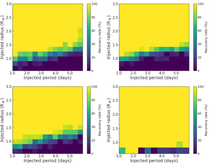
4.2. Results for TESS

Figure3presents results of injection-and-recovery tests for four stars observed in one sector by TESS. The four se-lected stars also are very quiet, non-variable stars. They have magnitudes of G=10.1, G=13.0, G=14.1, and G=15.0. Figure3shows that typically, „0.5 RC(G„10.0), „1.2 RC

(G„13.0), „1.9 RC(G„14.1), and „2.7 RC(G„15.0)

plan-ets can be retrieved from TESS one-sector light curves for the shortest orbital periods with a Á 90% recovery rate.

To appreciate the increase in detectability with mul-tisector observations, we performed similar tests on TIC 441713413 (G=13.07), which was observed in two sec-tors (S16 and S23), on TIC 220513363 (G=14.1), which was observed in three sectors (S1, S2, and S3), and on TIC 362103375 (G=13.04), which was observed in six sec-tors (S14, S15, S18, S22, S25, and S26). All stars were compared to results from one-sector-only tests (S16 for TIC 441713413, S1 for TIC 220513363, and S14 for TIC 362103375). Figure 4 and Table 3 present and compare the results of these experiments. The improvement in de-tectability from one to two sectors is barely perceptible and is noticeable only for orbital periods beyond 5 d. This is an important result because the majority of TESS targets were observed for one sector only during the primary mission (Table 1), and it will be reobserved for another one sec-tor in the extended mission. No significant improvement in detectability obtained from the one-sector primary mission (Fig.3) is therefore expected with one more sector data in the extended mission. The improvement from one to three sectors (TIC 220513363, see Table 3) and six sectors (TIC 362103375, see Fig. 4 and Table 3) is increasingly notice-able: We are now able to reach sub-Earth-sized objects up to 25 d with 6 sectors, for example, which was only possi-ble for an orbital period of 1 d (and below) with one sector only.

The effect of the data length on the minimum detectable radius can be described further. In an ideal case, the longer the data set, the smaller the planet that can be detected be-cause of the increased number of stacked transits. This im-proves the statistics and increases the signal-to-noise ratio (SNR). This is directly related to the working procedure of our transit-search algorithm (TLS, see Sect.3.2). However, the real nature of the light curves, which always present a level of noise that cannot be removed, means that we do not always have a clear improvement when more transits are stacked. This is in particular the case for the short orbital periods. Adding more transits does not always yield a vast improvement, providing there is already a large number of them. This is shown in Table 3 for orbital periods of 1 d, for instance, for KIC 8054179, EPIC 206535752, and TIC 441713413. For longer orbital periods, the effect is stronger because the increase in the number of stacked transits is relatively more important. For example, for the TESS sam-ple, the improvement in the minimum size of planets that can be detected with an orbital period of 15 d is remarkable when we expand our analysis from one sector to two (TIC 441713413), three (TIC 220513363), and six sectors (TIC 362103375).

Table 3. Minimum size of planets in units of RC that can be detected in typical light curves with a Á 90% recovery rate. All

stars have 0.175 ˘ 0.025 Rd and 0.47 ˘ 0.03 Md.

Object ID G Mag Data 1 d 5 d 15 d 25 d 35 d length (d) Kepler 8054179 14.3 90 0.3 0.5 0.8 1.0 1.2 30 0.5 0.6 1.0 – – 3353239 15.2 30 0.6 0.8 1.1 – – 5938349 16.1 30 0.7 1.1 2.0 – – 8889318 17.2 30 0.9 1.2 2.4 – – 5342213 17.7 30 1.2 1.7 3.2 – – K2 206535752 14.1 80 0.6 0.8 1.0 1.5 2.1 30 0.6 0.9 1.6 – – 211421561 14.9 30 0.7 1.4 1.9 – – 228682488 16.0 30 1.0 1.4 2.5 – – 251457058 17.1 30 1.4 2.3 3.4 – – 248840987 18.1 30 2.1 3.3 5.4 – – TESS 147283842 10.1 27 0.5 0.7 1.5 – – 362103375 13.0 27 1.0 1.7 2.0 – – 162 0.7 0.8 0.9 1.0 1.3 096949372 13.0 27 1.1 1.8 2.0 – – 441713413 13.1 27 1.3 1.7 2.0 – – 54 1.3 1.7 1.9 >10 >10 085400193 14.1 27 1.8 2.3 2.8 – – 220513363 14.1 27 1.6 1.8 2.7 – – 81 1.3 1.6 2.5 3.0 3.0 000008842 15.0 27 2.7 3.2 4.7 – –

To conclude this section, we mention that Fig.2´4 as well as Table3also allow us to assess the general reliability of our results for the Kepler, K2, and TESS light curves. While the detectability will (unavoidably) be dependent on the target (for similar magnitude) and/or sector or quarter (for similar data length; also because of the actual radius of the host star), the general comparison of the tests car-ried out here shows consistent trends. For example, the re-sults for three different stars with G„13.0 (TIC 096949372, 362103375, and 441713413) for one-sector TESS data of three different sectors are globally consistent.

5. CHEOPS performances for hot subdwarfs

Figure5displays typical light curves obtained by CHEOPS for four representative targets: (1) HD 149382, one of the brightest known sdB stars (G=8.9), which was not observed by TESS, Kepler, or K2; (2) CW83-1419-09 (G=12.0), and (3) TYC 982-614-1 (G=12.2), which represent typi-cal CHEOPS targets in terms of magnitude; and (4) TYC 499-2297-1, a fainter target of G=12.6, which exceeds the CHEOPS standard specifications. The light curves were processed using version 12 of the Data Reduction Pipeline (DRP;Hoyer et al. 2020).

These light curves were obtained with the aperture that offers the smallest root mean square of variation in count rates, which is generally the DEFAULT one (which has a ra-dius of 25 arcsec). Then, we evaluated how the flux was correlated with different parameters such as the time, the CHEOPS roll angle, the x–y centroids, the background,

and the contamination. This inspection was made with the pycheops4package (v0.9.6), which is developed specifically for the analysis of CHEOPS data. We thus decorrelated the light curves of any undesired trends by calculating the Bayesian information criteria (BIC) of each combination of trends under the assumption that the combination that in-duces the lowest BIC describes any trends best. We also removed outliers as required. After the light curves were decorrelated, we visually inspected them in the search for potential transits.

The hot subdwarf observations made by CHEOPS are fillers. This results in light curves spanning 1.5 to 5 hr (with gaps due to Earth occultations and/or passages through the South Atlantic Anomaly, but always with an efficiency of at least 60% for an orbit, and always less than 100%) separated by several days for a given target. This makes the applica-tion of injecapplica-tion-and-recovery tests as conducted in Sec-tion4 impractical. Our injection-and-recovery experiments were conducted with the TLS transit search tool, which is useful for long time-series observations such as those coming from Kepler, K2, or TESS. The power of TLS-based search-ing relies on the stacksearch-ing of many transits, which eventually increases the SNR of a given periodic signal. However, the CHEOPS light curves are short observational data sets, in which we expect to find single transits. To characterize the CHEOPS performance for hot subdwarfs, we therefore esti-mated the minimum planet size based on the transit depth that could be detected with an SNR of 5 assuming a transit

4

Fig. 3. Results of injection-and-recovery tests for four sdB stars observed in one sector by TESS: TIC 147283842 (G=10.1, top left panel), TIC 96949372 (G=13.0, top right panel), TIC 85400193 (G=14.1, bottom left panel), and TIC 000008842 (G=15.0, bottom right panel). 2500 injection-and-recovery tests were made for each star.

duration of 20 minutes (which is the typical duration for a „ 12 h orbital period) and for various typical stellar radii from 0.15 to 0.20 R_d.

The noise of the light curve is estimated with the pycheops package using the scaled noise method. It as-sumes that the noise in the light curve is white noise with a standard error b times the error values provided by the CHEOPS DRP. We then inject transits into the light curve and find the transit depth such that the SNR of the tran-sit depth measurement is 1. The trantran-sit model used for this noise estimate includes limb darkening, therefore we define the depth as D “ k2 _{, where k is the planet-star}

radius ratio used to calculate the nominal model. We can use a factor s to modify the transit depth in a nominal model m0calculated with approximately the correct depth to produce a new model mpsq “ 1 ` s ˆ pm0´ 1q. If the data are normalized fluxes f “ f1, . . . , fN with nominal er-rors σ “ σ1, . . . , σN , then the log-likelihood for the model given the data is

ln L “ ´ 1 2b2χ 2 ´1 2 N ÿ i“1 ln σ2_i ´ N ln b ´ N 2 lnp2πq, where χ2 “řN_i pfi´ 1 ´ spm0,i´ 1q 2 {σ2i. The maximum likelihood occurs for parameter values ˆs and ˆb such that

B ln L Bs ˇ ˇ ˆ s,ˆb“ 0 and B ln L Bb ˇ ˇ ˆ

s,ˆb“ 0, from which we obtain

ˆ s “ N ÿ i“1 pfi´ 1qpm0,i´ 1q σ2 i «_N ÿ i“1 pm0,i´ 1q2 σ2 i ff´1 and ˆ_{b “}a χ2_{{N .}

The standard errors on the eclipse depth if s « 1 are

σD“ Db «_N ÿ i“1 pmi´ 1q2 σ2 i ff´1{2 .

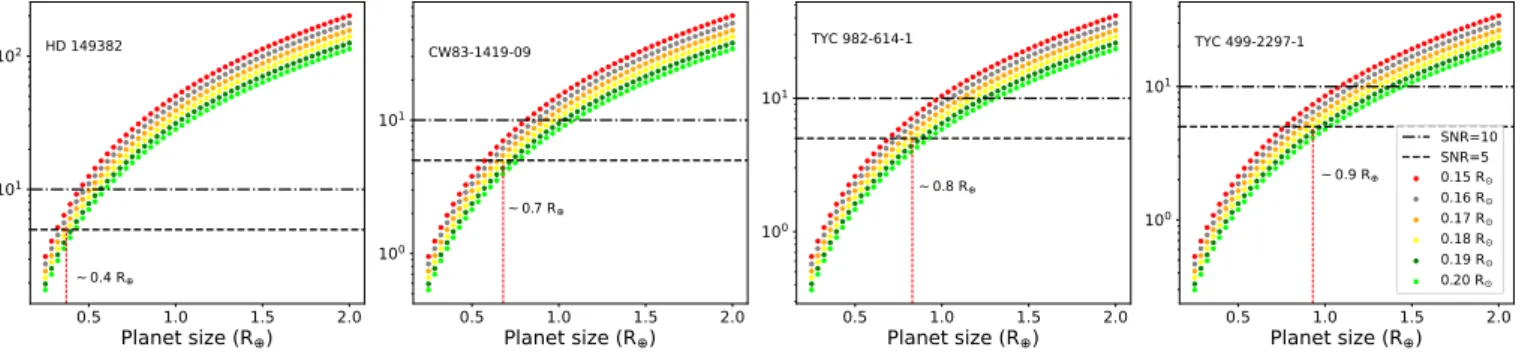
Figure 6 shows the minimum planet sizes that can be detected at SNR=5 for our four representative targets. For HD 149382, a „0.4 RC object (for a 0.18 Rd host) could

be detected at SNR=5 if it is transiting. CW83-1419-09 and TYC 982-614-1 exhibit typical results for CHEOPS targets, reaching detections of „0.7-0.8 RC objects.

Fi-nally, the fainter TYC 499-2297-1 could allow the detec-tion of a „0.9 RCobject. The minimum planet sizes for all

Fig. 4. Results of injection-and-recovery tests for stars observed in multiple sectors by TESS. Top panels: TIC 441713413 (G=13.07), one-sector data (left) and two-sector data (right). Bottom panels: TIC 362103375 (G=13.04), one-sector data (left) and six-sector data (right).

CHEOPS targets can be found in Table 2. They are given for a 0.18 Rd host and for SNR=5 in all cases.

Another important property to determine because of the filler nature of CHEOPS observations is which orbital peri-ods (and for which coverage of the orbit) are reached with the existing observations. This was measured by computing the phase coverage of a hypothetical planet in a range of periods. More precisely, we computed the percentage of the phase covered for each orbital period from Porb “0.001 d to

5 d in intervals of 0.001 d. To do this, we evaluated the phase coverage for a total of 5000 periods. Then, to aid interpret-ing the phase coverage at different periods, we binned the periods by 1.7 hr. To illustrate the current status of our observational program, we estimated the period at which a phase coverage of „80% is reached for each target, mean-ing that periods equal to or shorter than this would most likely be detected if the planet exists and transits. However, even when the probabilities are low, a hypothetical planet may still reside in the unexplored phase. Results for our four representative targets are presented in Fig.7. As of 19 December 2020, we found a phase coverage of „80% for or-bital periods of „0.47 d, „0.39 d, „ 0.68 d, and „0.54 d for our four representative cases HD 149384 (7 times two or-bits), CW83 1419-09 (4 times three oror-bits), TYC 982-614-1

(6 times three orbits), and TYC 499-2297-1 (6 times two orbits). The orbital periods reached for a phase coverage higher than 80% for the CHEOPS targets can be found in Table2.

In light of the results of the injection-and-recovery tests in the Kepler, K2, and TESS light curves, all CHEOPS targets with a minimum detectable planet size greater than Á 1.1RC have been suspended (see Table 2). These

tar-gets generally have fainter magnitudes, are located in a crowded field, or have a bright close contaminating ob-ject, which explains the poorer ability of detecting plan-ets around these objects. Another explanation is that some targets are pressure-mode (p-mode) sdB pulsators with a relatively high amplitude (this is the case for EC 15041-1409 and TYC 1077-218-1), which are not properly removed with our current detrending procedure (this is an improve-ment we aim to impleimprove-ment in the coming months). We instead chose to focus on the most promising targets for which planets below À 1.1RC can be detected because in

these cases, CHEOPS will notably contribute to increasing the number of targets for which we could detect planetary remnants (which are likely small, possibly disintegrating objects) around post-RGB stars. From Tables 1, A.1, and

0.04 0.06 0.08 0.10 0.12 0.14 0.16 BJD-2459020 0.999 1.000 1.001 Normalised flux HD 149382 Decorrelation model DRP data 0.04 0.06 0.08 0.10 0.12 0.14 0.16 BJD-2459020 Decorrelated data 5-min bin 0.200 0.225 0.250 0.275 0.300 0.325 0.350 0.375 0.400 BJD-2458962 0.996 0.998 1.000 1.002 1.004 Normalised flux CW83-1419-09 0.200 0.225 0.250 0.275 0.300 0.325 0.350 0.375 0.400 BJD-2458962 0.650 0.675 0.700 0.725 0.750 0.775 0.800 0.825 0.850 BJD-2459027 0.9950 0.9975 1.0000 1.0025 1.0050 Normalised flux TYC 982-641-1 0.650 0.675 0.700 0.725 0.750 0.775 0.800 0.825 0.850 BJD-2459027 0.26 0.28 0.30 0.32 0.34 0.36 0.38 BJD-2459064 0.990 0.995 1.000 1.005 1.010 Normalised flux TYC 499-2297-1 0.26 0.28 0.30 0.32 0.34 0.36 0.38 BJD-2459064

Fig. 5. Representative light curves of hot subdwarfs produced by CHEOPS. From top to bottom: HD 149382 (G=8.9) in its fifth visit, CW83 1419-09 (G=12.0) in its first visit, TYC 982-6141 (G=12.2) in its fourth visit, and TYC 499-2297-1 (G=12.6) in its fourth visit. In all cases, the raw light curves as processed by the DRP (gray dots) are displayed in the left panels, jointly with the best decorrelation model (orange line) found by means of the pycheops package. In the right panels, the decorrelated data (gray dots) with a 5-minute bin (blue dots) are shown. The y-scale is the same for each pair of right and left panels.

0.5 1.0 1.5 2.0 Planet size (R ) 101 102 SNR HD 149382 0.4 R 0.5 1.0 1.5 2.0 Planet size (R ) 100 101 CW83-1419-09 0.7 R 0.5 1.0 1.5 2.0 Planet size (R ) 100 101 TYC 982-614-1 0.8 R 0.5 1.0 1.5 2.0 Planet size (R ) 100 101 TYC 499-2297-1 0.9 R SNR=10 SNR=5 0.15 R 0.16 R 0.17 R 0.18 R 0.19 R 0.20 R

Fig. 6. Performances of CHEOPS on hot subdwarfs, assuming a single 20-minute transit. From left to right: HD 149382 (G=8.9), CW83-1419-09 (G=12.0), TYC 982-614-1 (G=12.2), and TYC 499-2297-1 (G=12.6). The minimum planet size for an SNR=5 and a 0.18 Rd host is indicated next to the vertical red line.

160 stars observed by Kepler and K2 (almost all of them for Kepler, and about two-thirds of them for K2) and about 50 stars from TESS (the very brightest ones, and those with G À 13.0 observed for at least about six sectors), will reach this minimum planet size. Statistically, only „40% of them are single hot subdwarfs, while in contrast, all CHEOPS targets have been chosen to be single hot subdwarfs (or, in a few cases, subdwarfs in wide binary systems) to the best of our knowledge.

The orbital periods reached by the CHEOPS filler obser-vations will remain modest (about 1 d orbital period with a 80% phase coverage by the end of the mission for most targets). However, these results are valuable for placing con-straints on the survival rates of planets that are engulfed in the envelope of their red giant host. These remnants, if present, are expected to have very short orbital periods because of the orbital decay of the orbit of the inspiraling planet inside its host star. It is noteworthy here that all of the five Earth-sized planets that are suspected around KIC

0 20 40 60 80 100 Ph as e C ov er ag e ( %

) HD 149382_{Period: 1.0 d -> Phase Coverage: 62.3 %}

Period: 2.0 d -> Phase Coverage: 33.3 % Period: 3.0 d -> Phase Coverage: 23.2 % ~80% of coverage reached at: ~0.47 d

0 20 40 60 80 100 Ph as e C ov er ag e ( %

) CW83-1419-09_{Period: 1.0 d -> Phase Coverage: 46.0 %}

Period: 2.0 d -> Phase Coverage: 25.6 % Period: 3.0 d -> Phase Coverage: 17.5 % ~80% of coverage reached at: ~0.39 d

0 20 40 60 80 100 Ph as e C ov er ag e ( %

) TYC 982-614-1_{Period: 1.0 d -> Phase Coverage: 64.4 %}

Period: 2.0 d -> Phase Coverage: 37.4 % Period: 3.0 d -> Phase Coverage: 22.0 % ~80% of coverage reached at: ~0.68 d

0 1 2 3 4 5 Period (days) 0 20 40 60 80 100 Ph as e C ov er ag e ( %

) TYC 499-2297-1_{Period: 1.0 d -> Phase Coverage: 55.6 %}

Period: 2.0 d -> Phase Coverage: 34.3 % Period: 3.0 d -> Phase Coverage: 19.8 % ~80% of coverage reached at: ~0.54 d

Fig. 7. Phase coverage (in percent) as a function of orbital period reached after one season of observations with CHEOPS. From top to bottom panel: HD 149382 (7x2 orbits), CW83 1419-09 (4x3 orbits), TYC 982-614-1 (6x3 orbits), and TYC 499-2297-1 (6x2 orbits). In all cases, the blue lines represent the full range of 5000 periods we explored, and the orange lines show the binning at each „1.7 hr. The orbital periods for which the phase coverages are „80% are marked with dotted vertical red lines.

05807616 and KIC 10001893 have orbital periods of only a few hours (Charpinet et al. 2011; Silvotti et al. 2014), and all known sdB+red dwarf or brown dwarf post-CE bi-naries have orbital periods below 1 d (Schaffenroth et al. 2018, 2019,2021). Finally, CHEOPS provides an excellent opportunity of observing very promising targets, such as HD 149382, which have not been observed by Kepler, K2, or TESS.

6. Conclusions and future work

This paper presented our project that searches for transit-ing planets around hot subdwarfs. While no such planetary transit have been found to date, high-quality photometric light curves are now available for thousands of hot subd-warfs from the Kepler, K2, TESS, and CHEOPS space mis-sions (the harvest is continuing for these last two mismis-sions).

By having experienced extreme mass loss on the RGB, these small stars (0.1-0.3 Rd) constitute excellent targets based

on which the question of the evolution of planetary sys-tems directly after the first-ascent red giant branch can be addressed. Hot subdwarfs also offer the potential of obser-vationally constraining the existence of planetary remnants, that is, planets that would have survived (even partially as a small, possibly disintegrating, very close object) being en-gulfed in the envelope of their red giant host star. Not only does the small star size enable the detection of small rem-nant objects, but the ejection of the envelope may even be the reason of the survival of such remnants by stopping the spiraling-in inside the host star. Hot subdwarfs may there-fore offer the outstanding opportunity to study the interior of giant planets, whose exact structure is uncertain, even for Jupiter (Wahl et al. 2017, and refererences therein).

We first listed the hot subdwarfs observed by Kepler, K2, TESS, and CHEOPS. We then performed injection-and-recovery tests for a selection of representative targets from Kepler, K2, and TESS, with the aim to determine which transiting bodies in terms of object radius and or-bital period we will be able to detect in these light curves with our tools. For CHEOPS targets, given the filler nature of the observations (they are carried out when CHEOPS has no time-constrained or higher-priority observations), we di-rectly estimated the minimum planet size detectable from the SNR of the light curves, and then computed the orbital periods that are covered for a given phase coverage. For comparison purposes, we considered the same host star in all cases.

Objects smaller than „1RC can be detected (if

exist-ing and transitexist-ing) for the shortest orbital periods (about 1 d and below) in most of the Kepler, K2, and CHEOPS targets. Values comparable to those for our Moon („0.3 RC) can be achieved in the best cases. This performance

of reaching sub-Earth-sized objects is obtained only for the very few brightest TESS data, as well as for stars with G À 13 that are observed for a significant number (Á 6) of sectors. Altogether, we estimate that we will be able to de-tect planets smaller than the Earth for about 250 targets for orbital periods shorter than 1 d, if they exist. Given the relatively high probability of transits for very close ob-jects (« 5% at 1 d orbital period), our results demonstrate that we will be able to observationally determine whether planets are able to survive being engulfed in the envelope of their host star. Hot subdwarfs represent a short phase of stellar evolution („ 150 Myr for the core-He burning, i.e., EHB, phase, and about 10% of that time for post-EHB evolution; Heber 2016), which renders the formation of second-generation planets unlikely, in particular in light of the harsh environment for planet formation around a hot subdwarf. Migration of bodies at greater distances that were not engulfed in the envelope of the red giant host would be possible for the oldest hot subdwarfs (Mustill et al. 2018), although their lifetime is likely too short for a com-plete circularization of the orbit. Dedicated computations will be required, as those carried out for the planets and remnants discovered around white dwarfs (Veras & Fuller 2020, and references therein).

Our tests also provided a series of representative re-sults for the detection of larger planets at greater distances. TESS targets will provide the most important cohort for the final goal of this project, which is to provide

statisti-cally significant occurrence rates of planets as a function of object radius and orbital period around hot subdwarfs.

Our main pipeline for the search for transit events around hot subdwarfs, SHERLOCK, has already been suc-cessfully applied in a number of cases (Pozuelos et al. 2020;

Demory et al. 2020). However, several implementations are being developed that are especially relevant given the na-ture of our targets. The first improvement involves more efficient detrending for pulsating stars (see, e.g., Sowicka et al. 2017), in particular, high-frequency p-mode hot sub-dwarf pulsators, which have relatively high amplitudes that can hinder the detection of shallow transits. Second, we in-clude in SHERLOCK a model for comet-like tails of disin-tegrating exoplanets, which highly differ from the typical shape of transiting exoplanets (see, e.g., Brogi et al. 2012;

Rappaport et al. 2012;Sanchis-Ojeda et al. 2015;Kennedy et al. 2019).

When a transit event in the light curves is identified that successfully passes all the thresholds and the vetting pro-cess, we will need to confirm the signal and associate it with a planetary nature by scheduling follow-up observations. In order to confirm transit events in light curves, we will trig-ger observations with our Liège TRAPPIST network ( Je-hin et al. 2011; Gillon et al. 2011) for the deepest signals (Á 2500 ppm), which consists of two 0.6 m telescopes at the La Silla (Chile) and Oukaïmeden (Morocco) observato-ries. For shallower transits, we will directly use CHEOPS, provided the target is sufficiently well visible from the or-bit of CHEOPS. When the transits are confirmed, a stellar, white dwarf, or brown dwarf origin will need to be ruled out based on RV measurements. We will first search for RV data in archives that are open to the community (such as the ESO archives) or within the hot subdwarf community. We will write proposals for appropriate spectrographs when necessary.

Finally, we will compute the occurrence rates of planets around hot subdwarfs by following a method similar to that ofvan Sluijs & Van Eylen(2018);Wilson et al. (2019). By comparing our results to these statistics for white dwarfs, to those for „0.8-2.3 Md main-sequence stars that are the

main progenitors of hot subdwarfs (e.g.,Mayor et al. 2011;

Howard et al. 2012;Fressin et al. 2013), as well as for sub-giants and RGB stars (Sato et al. 2008;Döllinger et al. 2009;

Jones et al. 2020), we will be able to appreciate the effect of the RGB phase alone on the evolution of exoplanetary systems.

Acknowledgements. We thank the anonymous referee for comments that improved the manuscript. The authors thank the Belgian Federal Science Policy Office (BELSPO) for the provision of financial support in the framework of the PRODEX Programme of the European Space Agency (ESA) under contract number PEA 4000131343. This work has been supported by the University of Liège through an ARC grant for Concerted Research Actions financed by the Wallonia-Brussels Federation. The authors acknowledge support from the Swiss NCCR PlanetS and the Swiss National Science Foundation. V.V.G. is a F.R.S.-FNRS Research Associate. M.G. is an F.R.S.-FNRS Senior Research Associate. St.C. acknowledges financial support from the Centre National d’Études Spatiales (CNES, France) and from the Agence Nationale de la Recherche (ANR, France) under grant ANR-17-CE31-0018. K.G.I. is the ESA CHEOPS Project Scientist and is responsible for the ESA CHEOPS Guest Observers Programme. She does not participate in, or contribute to, the definition of the Guaranteed Time Programme of the CHEOPS mission through which observations described in this paper have been taken, nor to any aspect of target selection for the programme. D.E. has received funding from the European Research Council (ERC) under the European Union’s Horizon 2020

research and innovation programme (project Four Aces; grant agreement No 724427). This project has been carried out in the frame of the National Centre for Competence in Research PlanetS supported by the Swiss National Science Foundation (SNSF). G.B. acknowledges support from CHEOPS ASI-INAF agreement n. 2019-29-HH.0. A.J.M. acknowledges funding from the Swedish Research Council (starting grant 2017-04945) and the Swedish National Space Agency (career grant 120/19C). A.C.C. and T.G.W. acknowledge support from STFC consolidated grant number ST/M001296/1. A.B. was supported by the SNSA. M.F. gratefully acknowledge the support of the Swedish National Space Agency (DNR 65/19, 174/18). S.H. acknowledges CNES funding through the grant 837319. S.C.C.B. acknowledges support from FCT through FCT contracts nr. IF/01312/2014/CP1215/CT0004. S.G.S. acknowledge support from FCT through FCT contract nr. CEECIND/00826/2018 and POPH/FSE (EC). This work was supported by FCT - Fundação para a Ciência e a Tecnologia through national funds and by FEDER through COMPETE2020 - Programa Operacional Competitivi-dade e Internacionalização by these grants: UID/FIS/04434/2019; UIDB/04434/2020; UIDP/04434/2020; PTDC/FIS-AST/32113/2017 POCI-01-0145-FEDER- 032113; PTDC/FIS-AST/28953/2017 POCI-01-0145-FEDER-028953; PTDC/FIS-AST/28987/2017 POCI-01-0145-FEDER-028987. O.D.S.D. is supported in the form of work contract (DL 57/2016/CP1364/CT0004) funded by na-tional funds through FCT. B.-O.D. acknowledges support from the Swiss National Science Foundation (PP00P2-190080). B.N.B. acknowledges funding through the TESS Guest Investigator Program Grant 80NSSC21K0364. We acknowledge support from the Span-ish Ministry of Science and Innovation and the European Regional Development Fund through grants 80435-C2-1-R, ESP2016-80435-C2-2-R, PGC2018-098153-B-C33, PGC2018-098153-B-C31, ESP2017-87676-C5-1-R, MDM-2017-0737 Unidad de Excelencia “María de Maeztu”- Centro de Astrobiología (INTA-CSIC), as well as the support of the Generalitat de Catalunya/CERCA programme. The MOC activities have been supported by the ESA contract No. 4000124370. I.R. acknowledges support from the Spanish Ministry of Science and Innovation and the European Regional Development Fund through grant PGC2018-098153-B- C33, as well as the support of the Generalitat de Catalunya/CERCA programme. X.B., Se.C., D.G., M.F. and J.L. acknowledge their role as ESA-appointed CHEOPS science team members. D.G. gratefully acknowledges financial support from the CRT foundation under Grant No. 2018.2323 “Gaseous or rocky? Unveiling the nature of small worlds”. P.F.L.M. acknowledges support from STFC research grant number ST/M001040/1. This project has been supported by the Hungarian National Research, Development and Innovation Office (NKFIH) grants GINOP-2.3.2-15-2016-00003, K-119517, K-125015, and the City of Szombathely under Agreement No. 67.177-21/2016. This paper includes data collected by the TESS mission. Funding for the TESS mission is provided by the NASA Explorer Program. Funding for the TESS Asteroseismic Science Operations Centre is provided by the Danish National Research Foundation (Grant agreement no.: DNRF106), ESA PRODEX (PEA 4000119301) and Stellar Astrophysics Centre (SAC) at Aarhus University. We thank the TESS team and staff and TASC/TASOC for their support of the present work. This work has made use of data from the ESA mission Gaia (https://www.cosmos.esa.int/gaia), processed by the Gaia Data Processing and Analysis Consortium (DPAC, https://www.cosmos.esa.int/web/gaia/dpac/consortium). Funding for the DPAC has been provided by national institutions, in particular the institutions participating in the Gaia Multilateral Agreement.

References

Allard, F., Wesemael, F., Fontaine, G., Bergeron, P., & Lamontagne, R. 1994, AJ, 107, 1565

Aller, A., Lillo-Box, J., Jones, D., Miranda, L. F., & Barceló Forteza, S. 2020, A&A, 635, A128

Baglin, A., Auvergne, M., Boisnard, L., et al. 2006, in 36th COSPAR Scientific Assembly, Vol. 36, 3749

Baran, A. S., Zola, S., Blokesz, A., Østensen, R. H., & Silvotti, R. 2015, A&A, 577, A146

Benz, W., Broeg, C., Fortier, A., et al. 2020, Experimental Astronomy [arXiv:2009.11633]

Beuermann, K., Dreizler, S., Hessman, F. V., & Deller, J. 2012, A&A, 543, A138