Using LES to Study Reacting Flows and Instabilities in Annular Combustion Chambers

This is an author-deposited version published in : http://oatao.univ-toulouse.fr/

Eprints ID : 8566

To link to this article : DOI:10.1007/s10494-011-9367-7 URL : http://dx.doi.org/10.1007/s10494-011-9367-7

O

pen

A

rchive

T

OULOUSE

A

rchive

O

uverte (

OATAO

)

OATAO is an open access repository that collects the work of Toulouse researchers and makes it freely available over the web where possible.

To cite this version :

Wolf, Pierre and Balakrishnan, Ramesh and Staffelbach, Gabriel and Gicquel, Laurent Y.M. and Poinsot, Thierry Using LES to Study Reacting Flows and Instabilities in Annular Combustion Chambers. (2012) Flow, Turbulence and Combustion, vol. 88 (n° 1-2). pp. 191-206. ISSN 1386-6184

Any correspondence concerning this service should be sent to the repository administrator: staff-oatao@listes.diff.inp-toulouse.fr

Using LES to Study Reacting Flows and Instabilities

in Annular Combustion Chambers

Pierre Wolf · Ramesh Balakrishnan · Gabriel Staffelbach · Laurent Y. M. Gicquel · Thierry Poinsot

Abstract Great prominence is put on the design of aeronautical gas turbines due to increasingly stringent regulations and the need to tackle rising fuel prices. This drive towards innovation has resulted sometimes in new concepts being prone to combustion instabilities. In the particular field of annular combustion chambers, these instabilities often take the form of azimuthal modes. To predict these modes, one must compute the full combustion chamber, which remained out of reach until very recently and the development of massively parallel computers. Since one of the most limiting factors in performing Large Eddy Simulation (LES) of real combustors is estimating the adequate grid, the effects of mesh resolution are investigated by computing full annular LES of a realistic helicopter combustion chamber on three grids, respectively made of 38, 93 and 336 million elements. Results are compared in terms of mean and fluctuating fields. LES captures self-established azimuthal modes. The presence and structure of the modes is discussed. This study therefore highlights the potential of LES for studying combustion instabilities in annular gas turbine combustors.

Keywords Combustion instabilities · Large Eddy Simulation · Annular gas turbines · Mesh resolution

P. Wolf (

B

e-mail: Pierre.Wolf@cerfacs.fr R. Balakrishnan

ALCF, Argonne National Laboratory, Argonne, IL, USA T. Poinsot

1 Introduction

Large Eddy Simulation (LES) has been the center of attention in the field of turbulent combustion in the last ten years [22, 24]. By giving access to the largest structures of reacting flows, LES has opened the path to full numerical studies of unsteady phenomena such as ignition [2] and combustion instabilities [13,26,29,31]. Using compressible LES solvers has also made studies of thermoacoustic phenomena possible [11,32]. The progressive development of complex geometry solvers, based on unstructured and hybrid meshes [19,20] has also opened a new path by allowing computations of real configurations and not just laboratory burners. Today, LES is used as a design tool in multiple companies when problems such as combustion instabilities must be studied and it is applied in the exact geometry and for the real operating parameters of the engine. Of course, classical Reynolds Averaged Navier Stokes methods are still used and will be continued to be used because they are fast, well adapted and tuned for many flows (especially wall-bounded flows) but they are complemented today by LES everytime a predictive simulation is required or a fully unsteady mechanism must be studied.

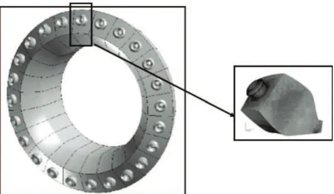
This paper describes recent progress in the field of LES in one specific class of problems: configurations which require the computation of a full annular cham-ber [9, 18, 30, 38, 39]. In gas turbines, most chambers use multiple sectors (15–24 typically), each one of them being fed by its own fuel injection system so that a usual simplification is to extract one of the burners, limit the study to 20 or 30 degrees of the whole chamber and assume axi-periodicity (Fig. 1). This simplification is used for laboratory experiments but also for CFD. It is a reasonable approximation but it fails in at least two cases: (1) ignition: to ignite a full annular combustor, the flame must propagate from sector to sector and no single sector approximation can be

Fig. 1 Simplifying the geometrical domain to study annular combustion chamber: single sector analysis

used and (2) azimuthal instability modes where combustion gets coupled with an azimuthal acoustic mode of the whole chamber, making single sector approximations impossible. The present paper focuses on the second case, and proposes to investigate the mesh dependency of LES and to describe the presence and structure of such modes in the simulations.

2 Large Eddy Simulation Models for Turbulent Combustion 2.1 High-order LES solver for compressible reacting flows

A fully compressible unstructured explicit code is used to solve the reactive multi-species Navier-Stokes equations [3–5,12,25]. A third order finite element scheme is used for both time and space advancement [7]. Sub-grid stress tensor is modeled by a classical non-dynamic Smagorinsky approach [35]. Boundary conditions are implemented through the NSCBC formulation [20, 23] and wall boundaries use a logarithmic law-of-the-wall formulation [29].

2.2 Chemical kinetics

Combustion is modeled using Arrhenius type reaction rates. Here a reduced one-step mechanism for JP-10/air flames is used [5, 6], JP-10 being a synthetic surrogate for kerosene (molecular formula: C10H16). Reduced one-step schemes can only guaran-tee proper flame speed predictions in the lean regime. For the target configuration, such a chemical scheme is not sufficient to predict proper flame positioning since the local equivalence ratio reaches a wide range of values. To circumvent such a shortcoming, the preexponential constant of the one-step scheme is adjusted versus local equivalence ratio to reproduce the proper flame speed dependency on the rich side [5, 14]. Note that prediction of emissions, e.g. N Ox, can not be achieved with such one-step mechanisms due to overestimation of the flame temperature and the non-inclusion of such intermediate species in the kinetics. Only five species are explicitly transported and solved for: J P10, O2,CO2,H2O and N2. To better capture flame/turbulence interactions, the Dynamic Thickened Flame (DTF) model is used [7, 8, 29]. The baseline idea of the DTF model is to detect reaction zones using a sensor and to thicken only these reaction zones, leaving the rest of the flow unmodified. Thickening depends on the local grid resolution and it locally adapts the combustion process to reach a numerically resolved flame front. The flame sub-grid scale wrinkling and interactions at the Sub-Grid Scale (SGS) level are thus supplied by an efficiency function [8,15]. The DTF approach has successfully been used in a wide variety of configurations [2,5,16,26,27,29,33].

3 Massively Parallel LES of Combustion

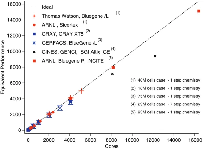
LES computations, performed on very large grids, for compressible reacting flows, require massively parallel capabilities. The solver used here is AVBP. Thanks to the use of the MPI library, this code offers a very good efficiency on a high number of processors. Figure 2 shows a perfect scaling of the speed-up up to 8,000 processors

16000 14000 12000 10000 8000 6000 4000 2000 0 Equivalent Performance 16000 14000 12000 10000 8000 6000 4000 2000 0 Cores Ideal

Thomas Watson, Bluegene /L (1) ARNL , Sicortex (1)

CRAY, CRAY XT5 (2) CERFACS, BlueGene /L(3)

CINES, GENCI, SGI Altix ICE (4) ARNL, Bluegene P, INCITE (5)

(1) 40M cells case - 1 step chemistry (2) 18M cells case - 1 step chemistry (3) 75M cells case - 1 step chemistry (4) 29M cells case - 7 step chemistry (5) 93M cells case - 1 step chemistry

Fig. 2 Speed up of LES solver on various machines

and a very reasonable speed up up to 16,000 processors [36,37]. More details on the parallel structure of the code can be found in [12]. This performance is the key to being able to compute the configurations described here.

4 Combustion Instabilities in an Annular Combustor 4.1 Configuration

This study focuses on an annular helicopter combustion chamber equipped with fifteen burners (Fig. 3). Each burner contains two co-annular counter-rotating swirlers. The fuel injectors are placed on the axis of the swirlers. To avoid uncertain-ties on boundary conditions the chamber casing is also computed. The computational domain starts after the inlet diffuser and ends at the throat of the high pressure stator. In this section, the flow is choked allowing for an accurate acoustic representation of the outlet. The air and fuel inlets use non-reflective boundary conditions [23]. The air flowing in the casing feeds the combustion chamber through the swirlers, cooling films and dilution holes, all of those being explicitly meshed and resolved. Multi-perforated walls used to cool the liners are taken into account by a homogeneous boundary condition [17]. To simplify the LES, fuel is supposed to be vaporized at the lips of the injector, leading to consider only gaseous phase. Thus, no model is used to describe liquid kerosene injection, dispersion and vaporization.

Fig. 3 Gas turbine geometry, boundary conditions and post-processing probes positions

Each burner is numbered starting with sector 1 placed at z = 0 and y > 0. The sector number increases clockwise. Specific data will be shown for the burners on two locations referred to as probe Ai and probe Bi (Fig.3) with i being the burner

index and going from 1 to 15. Type Aiprobes are located in the chamber casing and

Biprobes are located in each burner’s axis at the end of the burner.

The full chamber (fifteen sectors and burners) LES is initialized using a single sector LES with periodic boundary conditions which is then duplicated over the other fourteen sectors.

4.2 Mesh dependency

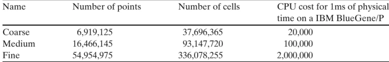
The choice of an adequate mesh for such a large domain is a critical question. It was investigated here by running three different levels of grids presented in Table 1.

Table 1 Characteristics of the unstructured meshes used for LES

Name Number of points Number of cells CPU cost for 1ms of physical time on a IBM BlueGene/P

Coarse 6,919,125 37,696,365 20,000

Medium 16,466,145 93,147,720 100,000

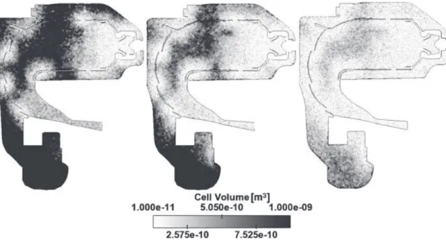
Fig. 4 Mesh resolution for the three grids, as obtained on a transversal cut passing through the

swirlers’ axis and showing only one sector. Left: coarse mesh, center: medium mesh and right: fine mesh

Figure4shows a detailed view of the mesh resolution on the three different grids for z = 0and y > 0. Grid topology is identical for all three meshes.

Due to the intrinsic properties of LES, two instantaneous LES fields may differ for various reasons [10,28,34]. However, one expects similar LES to converge towards the same statistics. Temporally averaged fields and standard deviation (RMS) fields are thus compared in this section to quantify the dependency of LES to mesh resolution in complex geometries.

The temporal averaging for the coarse and medium cases has been done over 13.8 ms.1 This averaging time corresponds to ten flow-through times, based on the mass flow rate and the primary zone volume, thus ensuring statistically converged values with regards to the main flow direction. However, due to the swirling flow at the exit of each burner and the azimuthal component of the flow emanating from the multiperforated walls, a weak but non-negligible azimuthal activity does exist in these annular configurations and leads to a very slow mean motion in the azimuthal direction: the mean azimuthal velocity in the chamber reaches values of the order of 10 m/s. An estimation of one flow-through time in the azimuthal direction is 0.15 s, which represents around 5 million iterations for the medium grid. Such a calculation would cost over 15 million CPU hours on a IBM BlueGene/P and remains out of reach, the fine grid simulation being even more costly. To improve

1_{Note that 4 ms of temporal averaging was achieved on the fine grid, due to the huge CPU cost of}

such a simulation. Mean quantities are reasonably converged, even with a shorter averaging time, although variances show a weaker agreement with the coarse and medium grids, as described in the following.

the statistics, a spatial sector-to-sector averaging over the fifteen sectors has been done: D ^f (x, t)E T = 1 15 15 X sector=1 1 T Z t0+_T t0 ^ f (x, t′ )dt′ (1) whereT is the time interval considered for temporal integration. The Favre notation ^f (x, t) is introduced to emphasize the fact that the statistics presented here are obtained from Favre-filtered quantities and might differ from the true turbulent statistics obtained in raw experimental measurements.

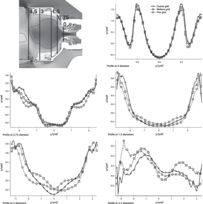
Figure5shows the mean axial velocity scaled by the inlet velocity on a transversal cut passing through the swirlers’ axis and showing the mean sector resulting from Eq. 1. The global flow topology between the three grids is very similar with a strong recirculating zone that extends from the nose of the injector to the primary dilution jets (highlighted as zone 1 on Fig. 5). High velocity regions at the exit of the swirler are retrieved with all meshes, as well as the upper and lower high speed parts of the primary zone (zone 1). The cooling films present similar shapes and levels. The main discrepancies between the fields are observed on the penetration of the primary dilution jets (highlighted as zones 2 on Fig.5) and on the downstream part of the recirculating zone, where the interaction with the primary dilution jets is intense. Figure 6 gives a more quantitative perception by displaying profiles of the mean axial velocity at five different axial positions from the exit of the swirler. Excellent agreement between the grids is found at the exit of the swirler. The next two profiles (0.75 and 1.5 diameters downstream) exhibit good agreement. The fourth profile shows differences between the three grids, especially on the lower part of the recirculating zone. The last profile is located near the primary dilution jets and confirms the discrepancies revealed by the axial velocity fields (Fig. 5—zones

Fig. 5 Mean axial velocity fields for the coarse (38 million cells—left), the medium (93 million cells—

Fig. 6 Profiles of the mean axial velocity at five different axial positions from the exit of the swirler:

0, 0.75, 1.5, 3 and 4.5 swirler diameters. Velocities are normalized by the inlet velocity and lengths are normalized by the swirler diameter

tagged 2). However, these differences have to be weighted against the fact that no combustion occurs along the line where this profile is measured (see Fig.8).

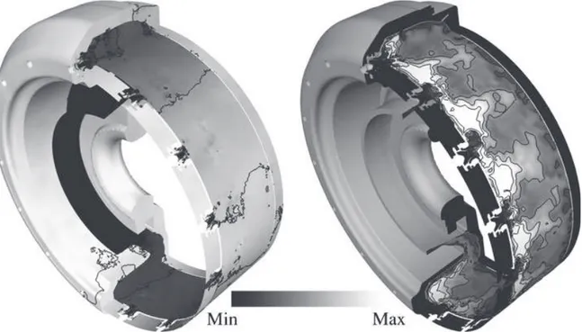
Figure7 presents the mean temperature field scaled by the inlet temperature on the plane defined by Fig. 5. Very good agreement is found between the three grids for this field. In particular, the mean flame position is identical, indicating proper behavior of the combustion model, with a flame that goes upstream almost to the injector nose. The thermal boundary layers created by the multiperforated walls and the cooling films are retrieved on all grids. As for the mean axial velocity fields, some dissimilarities between the meshes are seen on the penetration of the primary dilution jets.

Spatial distributions of the mean reaction rate are shown on Fig.8. As underlined previously by the mean temperature field, combustion occurs in the same region for

Fig. 7 Mean temperature fields for the coarse (38 million cells—left), the medium (93 million

cells—center) and the fine (336 million cells—right) grids. Temperatures are normalized by the inlet temperature

all three meshes. Peak values of the mean reaction rate are localized in two identical positions: very close to the lips of the separator and in the corners of the front of the primary zone. The reactive front is thinner as the mesh resolution increases, due to the nature of the DTF model, which depends on the local grid resolution and decreases thickening when the resolution increases.

Fig. 8 Mean reaction rate fields for the coarse (38 million cells—left), the medium (93 million cells—

Fig. 9 Probability density

function of local equivalence ratio in reacting zones on the coarse (38 million cells), the medium (93 million cells) and the fine (336 million cells) grids 2.0 1.5 1.0 0.5 0.0 Probability density 2.0 1.0 0.0 Equivalence ratio Coarse Medium Fine

Figure 9 gives more insights on the way combustion occurs by showing the probability density function (PDF) of the instantaneous resolved equivalence ratio in reacting zones. PDFs obtained on all three meshes are almost similar. Most of the combustion takes place in lean premixed zones, with a strong peak at an equivalence ratio of φmin. This emphasizes the proper use of the fitted one-step chemical scheme as most flame elements burn under lean conditions, where such a mechanism is suitable. Another peak is located at φ = 1 and stems from the presence of diffusion flamelets. A weaker peak appears around φmax and corresponds to rich premixed flames created close to the fuel injection.

Thickening is the central parameter in the DTF model. A major advantage of this model is that it converges to DNS when the mesh is sufficiently fine. At the Reynolds numbers considered for this study (Re = 55,000 based on the bulk velocity through the swirlers and the height of the chamber) and for the flame thickness (less

0.005 0.004 0.003 0.002 0.001 0.000 Percentage of points 80 60 40 20 Thickening Coarse Medium Fine

Table 2 Behavior of the DTF model on the three grids

Name Points affected by thickening Maximum thickening Mean thickening

Coarse 18.34% 81.5 18.77

Medium 14.93% 62.5 15.28

Fine 9.18% 44.8 10.70

than 0.05 mm) at this pressure, DNS is still impossible. However, the comparison of the flame thickening factors (Fig. 10) shows that increasing the number of mesh points decreases the mean thickening factor significantly. Note that the shape of the distribution remains similar on all meshes (apart from shifting towards lower thickening factors proportionally to the increase in resolution), indicating that the model behaves similarly on the three grids. Table2gives the percentage of the total grid points that are affected by thickening (i.e. where the flame is localized), the maximum thickening factor and its mean value. Even if the flame is obviously better resolved on the fine grid, drawing less stress on the DTF model, the combustion regime appears to be the same for the three cases.

4.3 Description of azimuthal mode

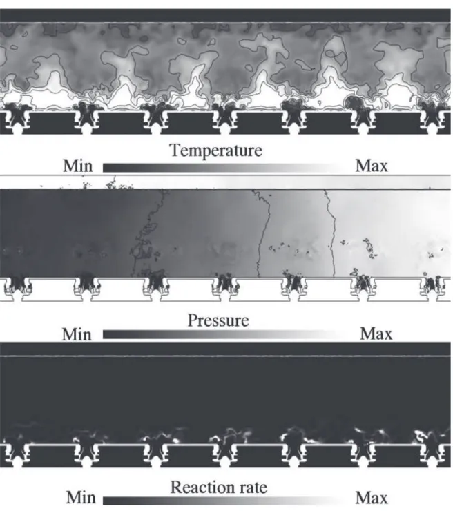
A snapshot of the temperature field on a cylindrical plane passing through the Bi

probes is displayed on Fig.11, along with the pressure field that exhibits the presence of azimuthal pressure waves. A direct observation of this field versus time (not shown here) reveals that, when the limit cycle is reached in LES, the flames oscillate azimuthally, moving from left to right at a frequency close to 750 Hz. This azimuthal

Fig. 11 Flow visualization. Left Pressure field with pressure isocontours. Right Temperature field

motion is accompanied by an axial displacement of all flames displayed in Fig. 12. This figure shows instantaneous temperature and pressure fields which reveal that the flame distances to the burners exit planes change: certain flames are very close to the burners (left side of Fig.12) while others are lifted (right side of Fig.12). This pattern oscillates at the frequency of the azimuthal mode.

To check the mesh dependency of the acoustic mode, the simulation has been run on the coarse mesh before being continued on the fine grid. Figure 13 displays the pressure fluctuations at probe B1. The frequency and amplitude of the perturbations are similar, showing that the mode captured by LES depends weakly on the mesh.

Fig. 12 Detailed view of half of the burners at an instant. Top Temperature field with temperature

Fig. 13 Mesh dependency

tests: pressure perturbations at probe B1. The simulation is

run on the coarse mesh (solid line) until t = 0.2215 ms. It is then continued on the fine grid (dashed line) Pressure 0.230 0.228 0.226 0.224 0.222 0.220 0.218 0.216 Time (s)

Figure14shows the time variations of the transverse velocity component for probe A1 and the first cycle of the azimuthal mode. When the LES begins on the full combustor geometry, a strong oscillation of the transverse velocity component ap-pears at 750 Hz. This frequency matches the value of the first azimuthal mode which can be obtained with a Helmholtz solver using the mean temperature distribution in the combustor [1, 21] and has also been identified with pressure transducers on the real burner. It can as well be estimated simply by : f = c

2πr where c is the sound

speed in the chamber and r the chamber radius. Here c ≈ 900 m.s−1

, r ≈ 0.2 m so that f ≈ 720 Hz which is close to the observed LES value of 750 Hz.

The reduced temperature (_TmeanT ) signals on probes B1, B6and B9confirm that the flames periodically flash back into the burners (Fig. 15). The flow rate fluctuations control the flame response and the heat release perturbation. Further analysis [38,40] show that all burners react in the same way to this flow rate fluctuation: the azimuthal instability coincides with a mode which is driven by the azimuthal shape of the annular chamber but it is also connected to purely longitudinal oscillations in each sector. The flow rate oscillations in each burner induces an unsteady reaction rate

Fig. 14 Transverse velocity

component at probe A1 0.04 0 -4 Azimuthal velocity [m/s] -3 -2 -1 0 1 2 3 Time [s] 0.02

Fig. 15 _TmeanT over time for probes B1, B6and B9

B9

B6

B1

T/Tmean [ ]

Time [s]

T/Tmean [ ]

T/Tmean [ ]

which then feeds the azimuthal mode. These fluctuations also lead to periodic flashback of the flames into the injectors, a dangerous mode of operation. To conclude, LES provides multiple new information on these types of unstable modes and suggests methods to control them.

5 Conclusions

Combustion instabilities, which can dramatically alter correct operation of engines, are a crucial issue today. Large Eddy Simulation (LES) is a very promising path to apprehend thermo-acoustic instabilities in complex geometries. An investigation of the capability of LES to predict such complex annular configurations is proposed. The flow field is shown to be reasonably mesh independent. Present parallel com-puters thus allow the LES of complete annular combustion chambers and the study of phenomena which were impossible to simulate up to now. Azimuthal combustion instability modes can be reproduced numerically, considerably saving time and cost compared to real experiments. Furthermore, such modes are shown to be equally captured with three mesh resolutions ranging from 38 to 336 million cells.

Acknowledgements This research used resources of the Argonne Leadership Computing Facility at Argonne National Laboratory, which is supported by the Office of Science of the U.S. Department of Energy under contract DE-AC02-06CH11357. The authors thank GENCI (Grand Equipement National de Calcul Intensif) and CINES (Centre Informatique National de l’Enseignement Supérieur) for providing part of the computing power necessary for these simulations. The support of Turbomeca (Dr. C. Bérat and Dr. T. Lederlin) is also acknowledged. This research is partly supported by the ANR under the project “SIMTUR” ANR-07-CIS7-008.

References

1. Benoit, L., Nicoud, F.: Numerical assessment of thermo-acoustic instabilities in gas turbines. Int. J. Numer. Methods Fluids 47(8–9), 849–855 (2005)

2. Boileau, M., Staffelbach, G., Cuenot, B., Poinsot, T., Bérat, C.: LES of an ignition sequence in a gas turbine engine. Combust. Flame 154(1–2), 2–22 (2008)

3. Boudier, G., Gicquel, L.Y.M., Poinsot, T., Bissières, D., Bérat, C.: Comparison of LES, RANS and experiments in an aeronautical gas turbine combustion chamber. Proc. Combust. Inst. 31, 3075–3082 (2007)

4. Boudier, G., Staffelbach, G., Gicquel, L., Poinsot, T.: Mesh dependency of turbulent reacting Large-Eddy Simulations in a gas turbine combustion chamber. In: ERCOFTAC (ed.) QLES (Quality and reliability of LES) Workshop. Leuven, Belgium (2007)

5. Boudier, G., Gicquel, L.Y.M., Poinsot, T., Bissières, D., Bérat, C.: Effect of mesh resolution on large eddy simulation of reacting flows in complex geometry combustors. Combust. Flame

155(1–2), 196–214 (2008)

6. Boudier, G., Lamarque, N., Staffelbach, G., Gicquel, L., Poinsot, T.: Thermo-acoustic stability of a helicopter gas turbine combustor using Large-Eddy Simulations. Int. J. Aeroacoust. 8(1), 69–94 (2009)

7. Colin, O., Rudgyard, M.: Development of high-order taylor-galerkin schemes for unsteady cal-culations. J. Comput. Phys. 162(2), 338–371 (2000)

8. Colin, O., Ducros, F., Veynante, D., Poinsot, T.: A thickened flame model for Large Eddy Simulations of turbulent premixed combustion. Phys. Fluids 12(7), 1843–1863 (2000)

9. Fureby, C.: LES of a multi-burner annular gas turbine combustor. Flow Turbul. Combust. 84(3), 543–564 (2010)

10. Ghosal, S., Moin, P.: The basic equations for the large eddy simulation of turbulent flows in complex geometry. J. Comput. Phys. 118, 24–37 (1995)

11. Giauque, A., Selle, L., Poinsot, T., Buechner, H., Kaufmann, P., Krebs, W.: System identification of a large-scale swirled partially premixed combustor using LES and measurements. J. Turbul.

6(21), 1–20 (2005)

12. Gourdain, N., Gicquel, L., Montagnac, M., Vermorel, O., Gazaix, M., Staffelbach, G., Garcia, M., Boussuge, J., Poinsot, T.: High performance parallel computing of flows in complex geometries: I. Methods. Comput. Sci. Disc. 2, 015003 (2009)

13. Huang, Y., Sung, H.G., Hsieh, S.Y., Yang, V.: Large Eddy Simulation of combustion dynamics of lean-premixed swirl-stabilized combustor. J. Propuls. Power 19(5), 782–794 (2003)

14. Légier, J.P.: Simulations numériques des instabilités de combustion dans les foyers aéronau-tiques. Phd thesis, INP Toulouse (2001)

15. Légier, J.P., Poinsot, T., Veynante, D.: Dynamically thickened flame LES model for premixed and non-premixed turbulent combustion. In: Proc. of the Summer Program, pp. 157–168. Center for Turbulence Research, NASA Ames/Stanford University (2000)

16. Martin, C., Benoit, L., Sommerer, Y., Nicoud, F., Poinsot, T.: LES and acoustic analysis of combustion instability in a staged turbulent swirled combustor. AIAA J. 44(4), 741–750 (2006) 17. Mendez, S., Nicoud, F.: Adiabatic homogeneous model for flow around a multiperforated plate.

AIAA J. 46(10), 2623–2633 (2008)

18. Moeck, J.P., Paul, M., Paschereit, C.O.: Thermoacoustic instabilities in an annular rijke tube. In: Proceedings of ASME Turbo Expo 2010, pp. 1–14 (2010)

19. Moin, P., Apte, S.V.: Large-Eddy Simulation of realistic gas turbine combustors. AIAA J. 44(4), 698–708 (2006)

20. Moureau, V., Lartigue, G., Sommerer, Y., Angelberger, C., Colin, O., Poinsot, T.: Numerical methods for unsteady compressible multi-component reacting flows on fixed and moving grids. J. Comput. Phys. 202(2), 710–736 (2005). doi:10.1016/j.jcp.2004.08.003

21. Nicoud, F., Benoit, L., Sensiau, C.: Acoustic modes in combustors with complex impedances and multidimensional active flames. AIAA J. 45, 426–441 (2007)

22. Pitsch, H.: Large Eddy Simulation of turbulent combustion. Annu. Rev. Fluid Mech. 38, 453–482 (2006)

23. Poinsot, T., Lele, S.: Boundary conditions for direct simulations of compressible viscous flows. J. Comput. Phys. 101(1), 104–129 (1992). doi:10.1016/0021-9991(92)90046-2

24. Poinsot, T., Veynante, D.: Theoretical and numerical combustion, 2nd edn. R.T. Edwards, Philadelphia (2005)

25. Roux, S., Lartigue, G., Poinsot, T., Meier, U., Bérat, C.: Studies of mean and unsteady flow in a swirled combustor using experiments, acoustic analysis and Large Eddy Simulations. Combust. Flame 141, 40–54 (2005)

26. Roux, A., Gicquel, L.Y.M., Sommerer, Y., Poinsot, T.J.: Large Eddy Simulation of mean and oscillating flow in a side-dump ramjet combustor. Combust. Flame 152(1–2), 154–176 (2007) 27. Roux, A., Gicquel, L.Y.M., Reichstadt, S., Bertier, N., Staffelbach, G., Vuillot, F., Poinsot,

T.: Analysis of unsteady reacting flows and impact of chemistry description in Large Eddy Simulations of side-dump ramjet combustors. Combust. Flame 157, 176–191 (2010)

28. Sagaut, P.: Large Eddy Simulation for Incompressible Flows. Springer, New York (2002) 29. Schmitt, P., Poinsot, T., Schuermans, B., Geigle, K.P.: Large-Eddy Simulation and experimental

study of heat transfer, nitric oxide emissions and combustion instability in a swirled turbulent high-pressure burner. J. Fluid Mech. 570, 17–46 (2007). doi:10.1017/S0022112006003156

30. Schuermans, B., Paschereit, C., Monkiewitz, P.: Nonlinear combustion instabilities in annular gas-turbine combustors. In: 44th AIAA Aerospace Sciences Meeting and Exhibit, Reno, NV, USA (2006)

31. Selle, L., Lartigue, G., Poinsot, T., Koch, R., Schildmacher, K.U., Krebs, W., Prade, B., Kaufmann, P., Veynante, D.: Compressible Large-Eddy Simulation of turbulent combustion in complex geometry on unstructured meshes. Combust. Flame 137(4), 489–505 (2004)

32. Selle, L., Benoit, L., Poinsot, T., Nicoud, F., Krebs, W.: Joint use of compressible Large-Eddy Simulation and helmoltz solvers for the analysis of rotating modes in an industrial swirled burner. Combust. Flame 145(1–2), 194–205 (2006)

33. Sengissen, A., Giauque, A., Staffelbach, G., Porta, M., Krebs, W., Kaufmann, P., Poinsot, T.: Large Eddy Simulation of piloting effects on turbulent swirling flames. Proc. Combust. Inst. 31, 1729–1736 (2007)

34. Senoner, J.M., García, M., Mendez, S., Staffelbach, G., Vermorel, O., Poinsot, T.: Growth of rounding errors and repetitivity of Large-Eddy Simulations. AIAA J. 46(7), 1773–1781 (2008) 35. Smagorinsky, J.: General circulation experiments with the primitive equations: 1. The basic

experiment. Mon. Weather Rev. 91, 99–164 (1963)

36. Staffelbach, G.: Simulation aux grandes échelles des instabilités de combustion dans les configurations multi-brûleurs. Phd thesis, INP Toulouse (2006)

37. Staffelbach, G., Poinsot, T.: High performance computing for combustion applications. In: Super Computing 2006. Tampa, Florida, USA (2006)

38. Staffelbach, G., Gicquel, L., Boudier, G., Poinsot, T.: Large Eddy Simulation of self-excited azimuthal modes in annular combustors. Proc. Combust. Inst. 32, 2909–2916 (2009)

39. Stow, S.R., Dowling, A.P.: Thermoacoustic oscillations in an annular combustor. In: ASME Paper. New Orleans, LA (2001)

40. Wolf, P., Staffelbach, G., Roux, A., Gicquel, L., Poinsot, T., Moureau, V.: Massively parallel LES of azimuthal thermo-acoustic instabilities in annular gas turbines. C. R. Acad. Sci. Méc. 337(6–7), 385–394 (2009)