Physical and land-cover variables influence ant functional groups and species diversity along elevational gradients

O

pen

A

rchive

T

OULOUSE

A

rchive

O

uverte (

OATAO

)

OATAO is an open access repository that collects the work of Toulouse researchers and

makes it freely available over the web where possible.

This is an author-deposited version published in :

http://oatao.univ-toulouse.fr/

Eprints ID : 10199

To link to this article : DOI:10.1007/s10980-013-9892-y

URL :

http://dx.doi.org/10.1007/s10980-013-9892-y

To cite this version : Bernadou, Abel and Céréghino, Régis and Barcet, Hugues and Combe,

Maud and Espadaler, Xavier and Fourcassié, Vincent. Physical and land-cover variables influence

ant functional groups and species diversity along elevational gradients. (2013) Landscape Ecology,

vol. 28 (n° 7). pp. 1387-1400. ISSN 0921-2973

Any correspondance concerning this service should be sent to the repository

administrator:

staff-oatao@listes-diff.inp-toulouse.fr

Physical and land-cover variables influence ant functional

groups and species diversity along elevational gradients

Abel Bernadou · Régis Céréghino ·

Hugues Barcet · Maud Combe · Xavier Espadaler · Vincent Fourcassié

Abstract Of particular importance in shaping spe-cies assemblages is the spatial heterogeneity of the environment. The aim of our study was to investigate the influence of spatial heterogeneity and environ-mental complexity on the distribution of ant functional groups and species diversity along altitudinal gradi-ents in a temperate ecosystem (Pyrenees Mountains). During three summers, we sampled 20 sites distributed across two Pyrenean valleys ranging in altitude from 1,009 to 2,339 rn by using pitfall traps and band collection. The environment around each sampling points was characterized by using both physical and land-cover variables. We then used a self-organizing map algorithm (SOM, neural network) to detect and

A. Bemadou (r:gJ) ·M. Combe · V. Fourcassié Centre de Recherches sur la Cognition Animale, UPS, CNRS, Université de Toulouse, 118 route de Narbonne, 31062 Toulouse cedex 9, France

e-mail: Abel.Bemadou@biologie.uni-regensburg.de

Present Address:

A. Bemadou

Evolution, Behaviour & Genetics-Biology 1, University of Regensburg, UniversitiitsstraBe 31, 93053 Regensburg, German y

R. Céréghino

EcoLab, Université Paul Sabatier, Batiment 4R1, 118 Route de Narbonne, 31062 Toulouse cedex 4, France

characterize the relationship between the spatial distribution of ant functional groups, species diversity, and the variables measured. The use of SOM allowed us to reduce the apparent complexity of the environ-ment to five clusters that highlighted two main gradients: an altitudinal gradient and a gradient of environmental closure. The composition of ant func-tional groups and species diversity changed along both of these gradients and was differently affected by environmental variables. The SOM also allowed us to validate the contours of most ant functional groups by highlighting the response of these groups to the environmental and land-cover variables.

Keywords Ants · Community ecology · Elevation gradient · Landscape heterogeneity ·Neural networks · Pyrenees

H. Barcet

UMR 5602 CNRS, Maison de la Recherche du Mirail, Geode, Université Toulouse II-Le Mirail, 5 Allées A Machado, 31058 Toulouse, France

X. Espadaler

Departament de Biologia Animal, de Biologia Vegetal i d'Ecologia, Facultat de Ciències, Universitat Autônoma de Barcelona, 08193 Bellaterra, Spain

Introduction

One of the main concerns in community ecology is to identify the environmental factors ( either biotic or abiotic) that shape species assemblages (Rosenzweig 1995). Of particular importance in this respect is the heterogeneity created by the variation of these factors. According to the hypothesis of habitat heterogeneity suggested by MacArthur and MacArthur (1961), species richness should increase with increasing structural complexity of the environment. This rela-tionship has indeed been found in many taxa, e.g. arthropods, birds, mammals, amphibians or reptiles (see Tews et al. 2004 for a review). Environmental heterogeneity can significantly influence not only species richness but also their relative distribution. The distribution of ants for example is significantly affected by the spatial heterogeneity generated by fire (Parr and Andersen 2008), anthropogenic disturbances (Kalif et al. 2001 ), habitat fragmentation (Vasconcelos et al. 2006), or grazing (Bestelmeyer and Wiens 1996). Natural gradients (e.g. altitude, latitude) are also a major source of spatial heterogeneity that can influ-ence the structure of species assemblages. Mountain-ous areas in particular are characterized by rapid changes in climate, soil, or vegetation, over relatively short distances (Korner 2007). They thus offer considerable landscape heterogeneity on a condensed area and are ideal for exploring the ecological mechanisms underlying spatial patterns in species richness and distribution.

In this study, we investigated the influence of spatial heterogeneity and environmental complexity along altitudinal gradients on the distribution of ant functional groups and species diversity across two Pyrenean valleys: one located in Andorra, on the Southern side of the Pyrenees (the Madriu-Perafita-Claror valley), and another located in France, on the Northern side of the Pyrenees (the Pique valley). The categorization of organisms into functional groups has been widely used in the study of animal communities (birds: Cody 1985; reptiles: Piank:a 1986). Species classification by functional groups reduces the appar-ent complexity of animal communities (Andersen

1997a) and thus facilitates the understanding of the

general principles that govern the functioning of ecosystems. Although the classification in functional groups has been used to study the ant fauna of Australia (Andersen 1995; Hoffmann and

Andersen 2003), South (Bestelmeyer and Wiens 1996) and North America (Andersen 1997a; Stephens and Wagner 2006), and Asia (Pfeiffer et al. 2003), this method has been rarely used to study the ant fauna of Europe (but see G6mez et al. 2003).

Environmental heterogeneity may act at multiple scales on animais, both spatially and temporally (Wiens 1989; Levin 1992). All ofthese scales however may not be relevant to understand how an animal interacts with its environment and the choice of the spatial scale at which to study environmental hetero-geneity should be consistent with its perception of the environment. This requires the selection of appropri-ate descriptive variables (Turner et al. 2001 ). Physical, chemical and biological data, however, are often difficult to analyze in an integrated way because they are complex, noisy, and vary and covary in a non-linear way (Lek and Guégan 2000). One solution is to use modeling techniques, such as artificial neural networks, that are able to take into account the complex structure of multi-dimensional datasets (Chon 2011). For example, the Self-Organizing Map algorithm (SOM, unsupervised neural network, Ko-honen 2001) is a powerful and well-suited tool to detect patterns in animal communities in relation to environmental variables (Lek and Guégan 2000). SOMs have been used in ecology to study mostly aquatic insect or fish communities (e.g. Compin and Céréghino 2007; ants: Groc et al. 2007; Delabie et al. 2009; Céréghino et al. 2010). In this study we used SOM to fulfill two main objectives: (1) to describe landscape spatial patterns along altitudinal gradients and to explore whether the apparent complexity of mountain environments can be reduced to a few simple elements and (2) to address the question ofhow ant functional groups and pattern of species diversity respond to the changes in land-cover and physical variables along these gradients.

Methods

Study area and sampling sites

Our study area was located in the Pyrenees, a mountain range located in south-west Europe and that is shared between Spain, France and the Principality of Andorra. Because of their orientation and geographie location, these mountains present considerable

climatic contrasts. The northem and western sides of the Pyrenees have an oceanic climate, with rainfall throughout the year, mild winters and cool summers. The southem side in contrast has a more continental climate, characterized by high solar radiation, torren-tial rains at equinoxes, large temperature variations, and very cold winters and dry summers.

Two valleys were sampled in this study: the Madriu-Perafita-Claror, in Andorra, and the Pique valley, in France. The Madriu-Perafita-Claror valley is a glacial valley located in the southeast part of Andorra that covers an area of 4,247 ha. The valley is oriented along an east-west axis and extends along an altitudinal gradient ranging from 1,055 to 2,905 m. The valley is well preserved: the production of timber has ceased in the 1950s' and since the 1980s' there has been almost no human intervention. Because of its state of preservation, the Madriu-Perafita-Claror val-ley has been registered in 2004 as W orld Heritage by UNESCO for its culturallandscape (www.unesco.org, see Madriu-Perafita-Claror valley). The Pique valley is a glacial valley predominantly oriented along a north-south axis, extending along an altitudinal gra-dient ranging from 650 to 3,116 m. lt is dominated by peak:s over 3,000 rn in altitude that lie on the border between France and Spain. This valley is part of the Natura 2,000 sites (www.natura2000.fr/); it covers an area of 8,251 ha divided into two main valleys (the Pique valley and the Lys valley).

We sampled ants at 20 sites (9 sites in the Madriu valley and 11 sites in the Pique valley) in July-August 2005 to 2007. To select the sampling sites, three main factors were considered: elevation, exposure, and type of vegetation cover. We sampled along an altitudinal gradient ranging from 1,300 to 2,300 rn for the Madriu valley, and from 1,000 to 2,300 rn for the Pique valley. Sampling could not be achieved over a larger altitu-dinal gradient, because of high anthropogenic pres-sures below 1,300 rn in the Madriu valley, and below 1,000 rn in the Pique valley. Locations higher than 2,300 rn were not sampled because ant species richness beyond this altitude is known to be very low (Glaser 2006). The two valleys were thus sampled on 62.5 and 61.4 %of their altitudinal range, for the Madriu and Pique valleys respectively. The different categories of vegetation covers considered for the selection of the sampling sites were: forest, meadow, seree and bushes. Table S 1 gives the main character-istics of the sampling sites for the two valleys.

Sampling methods and species identification

At each of the 20 sites, we used a variation of the ALL protocol (Agosti et al. 2000) to sample the ants. A 190 rn long line transect was traced and sampling points were placed on this line every 10 rn (mak:ing a total of 20 sampling points per site, yielding a total400 sampling points for the two valleys). The position of the sampling points were recorded by means of a GPS (Garmin® eTrex®) and subsequently loaded into DN A-GIS, a free geographie information system

(www .diva-gis.org).

Two collection methods were used to sample the ants at each sampling point: pitfall traps and hand collection. The pitfall traps consisted of plastic cups (diameter: 35 mm, height: 70 mm), filled to one-third of their height with ethylene glycol. The cups were buried so that their upper lip was flushed with the surface of the substrate. The pitfall traps were therefore set in action immediately and were left in place for 5-8 da ys (Table S 1 ). The pitfalls could not be operated for the same length of time because access to sorne of the transects was difficult and was sometimes pre-vented by adverse meteorological conditions. Pitfall trapping was supplemented by hand collecting around each sampling point at the moment the pitfalls were removed. Hand collecting consisted of one persan (the same persan for ali transects) picking up ali visible ants within a 2 rn radius around each trap during a maximum of 3 min. Ants were searched on the ground and in the vegetation; potential nesting sites were also inspected ( dead wood, undemeath stones/bark). The combination of pitfall and hand collecting sampling techniques is known to perform well in temperate regions (Groc et al. 2007). Winkler extractors were not used because the leaf litter is generally shallow (because of heavy rainfall, the presence of rocks, and high slope inclination) or relatively poor (particularly in coniferous forests) in mountainous environments. Ali ants collected at each sampling point were placed in plastic vials filled with 90 % ethanol. Once in the laboratory, ants were identified to the species level using available keys (Seifert 2007).

Because ants are social insects, a single sample may contain a high abundance of a rare species. Our analyses are therefore based on the species occurrence in the samples rather than on the number of individ-uals. A sampling point thus corresponds to the presence/absence of various species collected at a

sampling site by a pitfall trap or by hand collection around the pitfall or by both sampling methods. Consequently, the theoretical maximum of a species occurrence in a transect is 20.

Environmental variables and habitat characterization

The 20 sites sampled and the micro-environment around each pitfall were characterized by using four physical and eight land-caver variables. These 12 variables were chosen because they have been shawn to be consistently correlated with ant species richness in previous studies (for physical variables see for example: Kaspari et al. 2004; Sanders et al. 2007; Dunn et al. 2009a). The physical variables considered were: annual mean temperature (in °C), annual precipitation (in mm), elevation a.s.l (in rn) and slope. Annual mean temperature and annual precipitation were obtained from two GIS data layers (30 arc-seconds) of the WorldClim 1.4 database (Hijmans et al. 2005), whereas elevation was recorded directly in the field by a GPS. WorldClim computes temper-ature as a function of elevation, which means that ali points of a transect where characterized by the same temperature value in our study. The slope was characterized locally around each pitfall by the same persan throughout the whole study using the following scale: 0 (null to gentle slope ), 1 (moderate slope ), 2 (strong slope). To describe the area surrounding the pitfalls, digital photographs centered on each pitfall were taken. Then, on each photograph, we considered an area of 1 m2 centered on the pitfall and used an image analysis software to delineate the outline of the following land-caver variables within this area: shrub, bare rock/pebbles, dead wood/stump, litter, grass and bare soil. The percentage of area covered by each of these elements was then determined. In addition, we also noted the presence/absence of either a hardwood or coniferous canopy above each pitfall.

Ant functional groups

AU ant species collected in the Madriu and Pique valle ys were classified into five functional groups (see Table S2) according to the categorization proposed by Roig and Espadaler (2010). This latter is an adaptation for the lberian Peninsula and Balearic Islands of the classifica-tion used by Andersen (1995, 1997a, 2000) for

Australian and North American ants and on that used by Bestelmeyer and Wiens (1996) for South American ants. Given that sorne genera ( e.g. Formica andLasius in this study) are heterogeneous in terms of their ecology and behaviour, different functional groups sometimes share species of the same genus. The five following functional groups were distinguished:

Opportunists (0) these are, in general,

unspecial-ized species, whose distributions are strongly influenced by competition with other ants. Accord-ing to Andersen (2000), these species often span a large diversity of habitats. They predominate in areas where stress or disturbance limit ant diver-sity and biomass and thus in which behavioural dominance is low. In our study, this group is represented by species of the genus Formica and by species like Tapinoma erraticum and

Tetramo-rium impurum. T. erraticum was not classified as a Dominant Dolichoderinae because its societies are

small (Seifert 2007) with a much reduced worker number compared, e.g., to the polydomous species

T. nigerrimum.

- Social Parasites (SP): this group gathers species

that are either temporary (e.g. Lasius mixtus) or permanent (e.g. Strongylognatus testaceus) social parasites.

- Coarse Woody Debris Specialist (CWDS) this

group is represented by two species: Camponotus

herculeanus and C. ligniperda. These species nest

in stumps or tree trunks.

- Cold Climate Specialists/Shadow Habitats ( CCS/ SW): these species have their distributions

cen-tered on cold climate areas (Andersen 2000). They are generally characteristic of habitats where the abundance of dominant dolichoderines is low (Andersen 2000). This group is mainly represented in the Madriu and Pique valleys by the genera

Formica, Lasius and Myrmica. The ants of the

genus Myrmica were classified as CCS/SW rather than Opportunists because this genus is mainly present within mountainous, humid and grassy environments (Radchenko and Elmes 2010). - Cryptics ( C) the se species are small to tin y species.

This group is predominantly represented by myrmicines and ponerines that nest and forage within soil, litter and dead branches (Andersen

2000). These ants are mainly present in forested habitats. In our study, this group is represented by

the two genera Leptothorax and Temnothorax and by one species of the Lasius genus: L. flavus. Leptothorax and Temnothorax species were included in the Cryptics functional group because they have cryptic behaviour in the sense that they forage singly, move slowly and "have little interaction with other epigaeic ants" (Andersen

1995).

Data analysis

To estimate total ant species richness at the valley and transect levels and to evaluate the completeness of our samples, Chao2, a non parametric richness estimator, was calculated with the program EstimateS 7.5.2 (100 replicates) (Colwe112005).

We used the SOM Toolbox (version 2) for Matlab® developed by the Laboratory of Information and Computer Science at the Helsinki University of Technology (http:/ /www .cis.hut.fi/projects/somtool box/, see Vesanto et al. (1999) for practical instruc-tions). The SOM is an unsupervised learning procedure which transforms a set of multidimensional data into a two dimensional map subject to a topological con-straint (see Kohonen 2001 for details). The data are projected onto a rectangular grid composed of hexag-onal cells, forming a map (Giraudel and Lek 2001 ). The SOM plots the similarities of the data by grouping similar data items together as follows:

(i) Virtual samples (visualized here as hexagonal cells) are initialized with random samples taken from the input data set.

(ii) The virtual samples are updated in an iterative way: (1) a sample unit is randomly chosen as an input unit, (2) the Euclidean distance between this sample unit and every virtual sample is computed, (3) the virtual sample closest to the input unit is selected and called 'best matching unit' (BMU), and ( 4) the BMU and its neighbours are moved a bit towards the input unit.

The training is separated into two parts:

(i) Ordering phase (the 3,000 first steps): when this phase takes place, the samples are highly mod-ified in the wide neighbourhood of the BMU.

(ii) Tuning phase (7,000 steps): during this phase, only the virtual samples adjacent to the BMU are lightly modified. At the end of the training, the BMU is determined for each sample, and each sample is set in the corresponding hexagon of the SOM map. Neighbouring samples on the grid are expected to represent adjacent clusters of samples. Consequently, sampling points appearing distant in the modelling space ( according to physical and land-cover variables) represent expected differences among sampling points in real environmental characteristics. The self-organizing map for this study consists of two layers of neurons connected by weights: an input layer and an output layer. The input layer was composed of 12 neurons (one per variable) connected to the 400 sampling points. The output layer was composed of 98 neurons (see below) visualized as hexagonal cells organized on an array of 14 rows by 7 columns (Fig. la). The number of output neurons (map size) is important to detect the deviation of the data. If the map size is too small, it might not exp lain sorne important differences that should be detected (Compin and Céréghino 2007). Conversely, if the map size is too big, the differences are too small. We followed the procedure described in Park et al. (2003) and Céréghino and Park (2009): the network was trained with different map sizes (4-200 neurons) and we chose the optimum map size based on local minimum values for quantization and topographie errors. Quantization error is the average distance between each data vector and its BMU and, thus, measures map resolution. Topographie error repre-sents the proportion of ali data vectors for which 1 st and 2nd BMUs are not adjacent, and is used for the measurement of topology preservation The number of 98 output neurons retained for this study fitted well the heuristic rule suggested by Vesanto et al. (2000) who reported that the optimal number of map units is close to 5-Jn, where n is the number of samples. For each sampling point, we made a list of the different species collected and determined the values of the environ-mental variables characterizing the sampling point. To highlight the relationships between the different ant functional groups and the environmental variables, the number of species occurrences of each functional group was introduced into the SOM previously trained

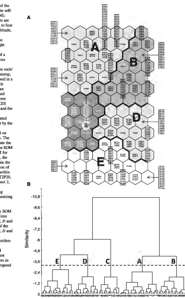
Fig. 1 Distribution of the sampling points on the self-organizing map (SOM). a The sampling points are distributed according to four physical variables (altitude, slope, mean annual temperature and mean precipitation) and eight land-cover variables variables (presence of a hardwood or coniferous canopy, percent area covered by shrub, bare rock/ pebbles, dead wood/stump, litter, grass and bare soil in a 1 m2 area around each pitfall). Altitude, mean annual temperature and mean precipitation were obtained by using a GIS software while slope and the eight environmental variables were estimated directly in the field or by the analysis of digital

photographs centered on each sampling points. The codes used to designate the sampling points on the SOM refer to the valley (M for Madriu, P for Pique), the transect number within the valley, and the location of the sampling points within the transect (e.g.: MT2P20, Madriu valley, Transect 2, sampling points 20). Neighboring sampling points on the self-organizing map share similar

environmental

characteristics. b The SOM units were classified into five clusters (A, B, C, D and

E). The boundaries of the five clusters (A, B, C, D and

E) were obtained by applying Ward's algorithm to the weights of the variables in the SOM hexagons. The smallest branches with numbers in the dendrogram correspond to the SOM neurons

A B

>

-·;::::: J!!

·e

i:i) -10,8 -9,6 -8,4 -7,2 -6 -4,8 -3,6

E

D

-2,4 -1,2 MTIP15 MT6P16 UTIP17 MT6P1G "''""' """"' """" """"' """" .,.,, .,.,, .,.,,

c

"""'' """" """" """" """" """"

A

B

with the four physical and the eight land cover variables that characterize each sampling point. Dur-ing the trainDur-ing of the map, we used a mask to give a null weight to the five functional groups, whereas physical and land-cover variables were given a weight of 1. Therefore, the search for the BMU was based on the 4 physical and 8land-cover variables only. Setting the mask value to zero for a given component (here for each of the five functional groups) removes the effect of that component on the map organization (Vesanto et al. 2000). The values and distributions of the functional groups were then visualized on the SOM previously trained with physical and land-cover vari-ables only and formed by the 98 hexagonal cells.

In a last step, Ward's algorithm was used to identify the boundaries between each cluster on the Kohonen map (Fig. 1 b ). The distributions of the number of species occurrences in each ant functional groups in the different clusters were compared using the

x

2 test for independent samples (Siegel and Castellan 1988). To further analyze the distribution of functional groups within each cluster, an analysis of residuals was performed (Siegel and Castellan 1988). This analysis tests the contribution of each functional group to each cluster. Moreover, it reveals whether a functional group is positively or negatively associated to a given cluster. We used a generalized linear mixed model (GLMM) with a Poisson error distribution to examine the variation in ant species richness per sampling point among the SOM clusters. To account for spatial autocorrelation among sampling points located in the same transects and in the same valley, the variable transect was nested within the variable valley and was entered as a random variable in the model. To assess the overall effect of the SOM clusters on species diversity we fitted a first model in which the SOM cluster variable was entered as a fixed effect categor-ical factor and the transect variable (nested within valley) was entered as a random effect categorical factor. We then fitted a second model with no fixed effects and compared the two models with a likelihood ratio test (Zuur et al. 2009). The different SOM clusters were then regrouped by removing non-significant factor levels in a stepwise a posteriori procedure (Crawley 2007). The models were fitted with the statistical software R 2.11.0 (R Development Core Team 2011) and the R-package lme4 (linear mixed-effects models using S4 classes, Bates et al.

2011) using the function glmer.

Results

Classification of sampling sites

Mter training the Kohonen map with the four physical variables and the eight land-cover variables, five clusters of sampling sites obtained from the SOM output were identified (Fig. la, b).

The SOM allowed us to identify two main gradients (Fig. 2 and Fig. S 1 ): a fust gradient extending from the lower right to the upper left corner of the map ( clusters D and E vs. cluster A, B and C), which corresponds to an altitudinal gradient ranging from low to high altitudes, and a second gradient, extending from the bottom to the top of the map (clusters C, D andE vs. cluster A and B), which corresponds to a gradient of environmental closure, ranging from closed to open areas.

Cluster B corresponds to sampling sites of medium elevations located in open areas, e.g. grassland areas (Fig. 2). Cluster A is equivalent to cluster B but for high elevation. It includes sampling sites typical of mountain environments, e.g. screes of high altitudes located on steep slopes. A large proportion of the sampling sites of cluster A is dominated by bare rocks and shrubs (Fig. 2). Clusters C and E correspond to sampling sites in forest areas: cluster E to low altitude forests dominated by hardwood, with a high ahun-dance of litter and dead wood, and cluster C to high altitude forests in which conifers are predominant. Note that for cluster E the sampling sites with high slopes are also characterized by bare soil. Cluster D corresponds to a transition area between hardwood forests and grasslands (Fig. 2).

Distribution of ant functional groups and species diversity

In total, 42 ant species were found in the two valleys. The number of species collected at each transect varied between 25 at 1,351 rn and 2 at 2,339 rn, and between 14 at 1,009 rn and 4 at 2,299 rn, for the Madriu and Pique valley respectively. The Chao2 estima tor indicated that between 66 and 100 % (mean± SD = 93.48 ± 10.89) of the expected max-imum number of species were collected for the 9 transects in the Madriu valley, and between 63 and 100 % (mean ± SD = 90.74 ± 12.29) for the 11 transects in the Pique valley using pitfall traps and

Altitude (m a.s.l) Slope (from 0 to 2)

Hardwood canopy (0/1) Coniferous canopy (0/11

0.998

Grass (%1 Sare soil (% 1

Fil-

l Gradient disaibution of each mVÛOIIIDeDtal variable 011 the 1raiDecl self-orgauizing map. A grayscale (datk = lligb

value.ligbt

=

low values) was used to viBualize the value of the variables. 1be SOM allows to derive two main gradients: an

a11itudiDal gradient rangiDg from.low (clusten D andE) to higb

band collecting. There was no relationship between these

values and

the duration of pitfall activity for the

Madriu

va11ey (Spearman's

rank

correlation:

r

=

-0.49, P

=

0.17,

n

=

9) or the Pique valley

(Spear-man's rank correlation:

r

=

0.15,

P

=

0.64,

n

=

11)

(Table S1).

The distribution of

the

:five functional groups on the

SOM previously trained with

the

physical and

land-caver variables are shown

m

Fig.

3

. With the

excep-tion of Social Parasites,

ali functional groups are

present

m

the :fi.ve clusters

of

the Kohonen map. The

Cold Climate Speci.alists/Shadow

Habitats is the

dominant functional group

m

most clusters (range:

Clusters

Litter (% 1 Dead wood 1 stump (% 1

7.4

3.71

0

Shrub(~·l Sare rock 1 pebbles (~.)

47.5

24.2

0.935

(clusteD

A.

B md C) altitudes, ami a gradient of enviroJJmcatal

closure. rangiDg from closed (cl.usters C, D aad E) to open

(clustcrs A and B) areas. See also Fig. Sl for the mean amrual

temperature IUid mean precipitation variables

44-58 %, mean:

56

%, Fig. 4a). The Opportunists is the

second largest group (range: 23-47 %, mean:

30 %), followed.

by

the Cryptics (range:

8-19 %,

mean: 11

%),

the

Coarse

Woody Debris Specialists

(range:

1-15 %, mean:

5

%) and the Social Parasites

(range: 0-3 %, mean: 1

%)

(Figs.

3

,

4a).

The distribution of species occurrences

m

each

functional group was not homogeneous across the :five

clusters

(j-

=

96.16, df

=

16, p

<

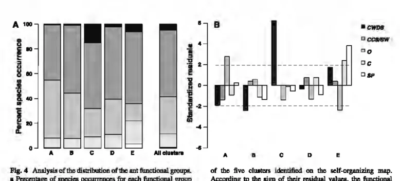
0.001).

The

Coarse

Woody Debris Specialists functional group

was signi:ficantly and positively associated with cluster

C (residuals

=

6.2, Figs.

3

,

4

b) and negatively

asso-ciated with cluster B {residual

=

-2.4, Figs.

3

,

4

b)

o.rr

0.1U

0

Fig. 3 Ant fuoctinnal groups. Visualization of the fi.ve ant

functi.oDal groups on the sclf-m:ganizing map traiDed with the four physieal and the eigbt Jand.cover variables. Each furu:tional

group bas its own disttilmtion pattern. The fnnctional groups

oc:cupying llimilar zone& on the map have a high probability to

Atoo

8

~10

....

:Il u

Seo

.1

i40

•

110

t.

0

A 8

c

D E Ali elu etant

Fig. 4 Analyail of the distribution of the ant func:tional groups. a Pm:entage of spccies DCC~~IIeDCes for earh functional group fouml in the Madriu and Pique valley. The pereeatagcs are givcu for eaclt of the fi.ve clusœrs idmtifi.ed by Ward's algoritbm on

the self-organizing map IIDCl for

an

clusterll grouped together.

b Residual values for the five ant functional groups fOUDd in the Madriu and Pique valley. The residual values are given for each

8

Opportwlllta

0

be associated and to be fouml in the 111111e area. A grayscale (ligbt = low values, dEk = bigh values) was used to visualize

the levet of pre$eDCC of eacb furu:tional group. Note that the

grayscak1 are different for eaclt functional group

B

----~---~--A Il

c

D E

of the fi.ve clUiters idmtifi.ed on the sclf-organizing map. Acconling to the sigll of their residual values, the func:tional groups may be posilivcly or negativcly associated with the

clustas. The two doUed. !iDes represent the significance

tbreshold at P

=

0.05. 0 opportunim, SP social parasites,

CWDS coane woody debris spcciali&t, CCSISW cold climate specialist8/8hadow habitats and C c::ryptics

and toalesse.rextenttocluster A(residual =

-1.8,

not significant. Figs. 3. 4b). This

functional

group is thus characteristic of woodland areas

and

is negatively associated with open areas. The Cold Climate Spe-cialists/Shadow Habitat and

Opporbmist

functional groups do not show any clear distribution pattern. They

are abundant

in ali clusters (Fig. 4a). The Social Parasites are signifi.cantly and positively associated with cluster B (œsiduals

=

3.8, Fig. 4b). The Cryptic group was significantly pœsent in cluster B (residu-ais= 2.3.

F1g.

4b)

and

is thus associated with the

presence of

litter and han\wood canopy.

The distribution

of

ant species ri.chness per sam-pling point

differed

signiftcantly among the five clusters (GLMM,

f

= 94.18,

df= 4,

p

<

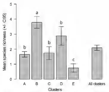
0.001). Cluster B bad the lowest ant species richness (mean ant species richness per sampling point

±Cio.9.s:

0.74

±

0.27) while clusters B (3.77

±

0.38) bad the

highest one (Fig. 5). Cluster D was only marginally significantly different from clusters A and C (GLMM,

z

value

=

1.93, p

=

0.052).

Dlscussion

ln

this

study we

used

a

Self-O.rganizing Map algorithm

to categorize 400 sampling points on the

basia of

12

5

~

4 ü

m

2 ·~ (/) c

8l

1 :2; 0

a

A B b

c

D E Ali clusters Clusters

Fig. 5 Ant speciea rlclmess. Mean 11UD1ber of ant speeies (::1:: Clo-95) per sampling poim for eaclt SOM cluster (A-E) 8lld

for ail clustas groupcd togedler. Significant differences in ant speçi.cs ric:Jmess between clusteD wme tested with a genaalized

linear mixed model (GLMM) with a Poisson eaor distribution. Different lettcrll above the error btJn indicate sigomcant differeDœs in mt species riclmess at P < 0.05

environmental variables characterizing the physical environment

and

the type

of

land-cover around each sampling point. The SOM algorithm :redu.ced the complexity of the database to fi.ve clusters of sampling points corresponding to high and low elevation grassland

areas,

hardwood and coniferous forests, and

a

transition

area

between hardwood forests and grasslands. These clusters highligb.t two main gradi-ents: an altitudinal gradient that mimics to a certain

extent the altitudinal zonation of vegetation found in the Pyrenees (Ninot et al. 2007)

and

a gradient

of

environmental closure. We then categorized the species

found

at the sampling points into nve functional groups and

used

the SOM map generated by the algmithm to stud.y the distribution of these groups in the environments sampled. Using this method, we were able to validate the contours of most functional groups by positively or negatively

corre-lating their disttibution with the environmental vari-ables measmed. The disttibution of ant functional groups changed along environmental gradients and was differently affec1ed by environmental variables. Finally. we examineA the disttibution

of

ant specles richness across the ôve clusters of sampling

points

identifi.ed by the SOM algorithm to fi.nd out the environmental characteristics associ.ated with low or high

ant

species diversity.

Three of

the fi.ve functional groups (Coarse Woody Debris Specialists, Sociol Parasites tmd the Cryptic) showed a clear pattern of

association with particular features

of

the environment such as the presence of litter and canopy. 1'hese tbree groups however represented only 31 % of the 42 species collected whereas the disttibution pattern of the two other functional groups ( Cold Climate Specialist/Shadow Habitat and OpportrmistJJ) that

represented 69 % of the total number of specles collected was much less clear. Our results show therefore

that the

disttibution of

the

ôve functional groups we

de1ined

change along environm.ental

gra-dients.

and that they

are thus

differently affected by

environmental variables. Assuming tbat species are more likely to reach neighboring areas than areas far apart

and

that neighboring sampling

points

tend to exhibit similar physical features, small-scale autocor-relatiom of ant assemblages were suggested from the SOM outputs (Figs. 1, 2, 3). However. almost ali ant functional groups (four out of fi.ve) were

present

within ali SOM clusters which shows that spatial autoco.rrelation alone cannot explain the SOM oulputs.

Indeed, if spatial autocorrelation were the only factor explaining the relationship between sampling points then each of the SOM elus ter would correspond to an ant functional group.

Why does the SOM analysis show such a discrep-ancy among functional groups in their pattern of association with environmental variables and why do in particular both the Cold Climate SpecialistJShadow Habitat and Opportunists functional groups appear to be so widely distributed in our sampling area? Two explanations could be provided. The fust explanation could be that this result reflects true particular biological traits of the species belonging to these groups. According to Andersen (1995, 1997a, 2000) the distribution of the Cold Climate Specialists/ Shadow Habitat species is centred on cool-temperate regions. In the two valleys we sampled, this group was represented by three genera: Formica, Lasius and

Myrmica. Most of the species of these genera are holarctic and are characteristic of the cold regions of the northern hemisphere (Bernard 1968). Their suc-cess in these regions is mainly due to specifie behavioural and/or physiological adaptive traits that allow them to resist to low temperatures (Heinze 1992; Maysov and Kipyatkov 2009). Since the whole area we sampled was located in a temperate mountainous region it should therefore come as no surprise that the Cold Climate Specialists/Shadow Habitat functional group was not found to be associated with any particular specifie environmental variable. As for the species belonging to the Opportunistic functional group, we found that they occupy a wide range of habitat but were particularly present in grassland areas of high altitudes, a relatively stressful environment for ants, both because of the low temperatures, charac-teristic of high altitudes, and of the scarcity of food (Andersen 2000).

A second and alternative explanation to the dis-crepancy found among functional groups in their pattern of association with environmental variables could be linked to the criteria used to define the functional groups. The criteria used to define the Cold Climate SpecialistJShadow Habitat and Opportunists functional groups could not be relevant to obtain clear patterns with the SOM analysis. As pointed out by Andersen (1997b) the definition of functional groups is scale-dependent and one should thus be cautious in using them in community ecolo gy studies. As a case in point Andersen (1997b) gives the example of the

mound-building species of the genus Formica. At a local scale, these species are behaviorally dominant throughout the Holarctic and they could thus be described as belonging to the dominant species functional group in local ant fauna (Andersen 1997b; Savolainen and VepsaHi.inen 1988). However, this dominance is limited to cool-temperate regions and at a global scale they would rather be considered as belonging to the group of cold-climate specialists. The importance of competition and dominance in ant community structure is thus scale dependent. The categorization in functional groups used in our study corresponds to that proposed by Roig and Espadaler (2010) to describe the ant fauna of the lberian Peninsula and Balearic Islands. Applied at the local scale of our study area, this categorization may not be discriminative enough (Andersen 1997b) and could conceal the response of sorne ant species to particular ecological variables. A solution could have been found in subdividing sorne of the functional groups we used (Bestelmeyer and Wiens 1996; Andersen 1997b). This could have increased the discriminative power of our analysis and as a consequence, clearer successional patterns in relation to environmental variables could have been revealed.

The ant species belonging to the Coarse Woody Debris Specialists and Cryptic functional groups were significantly and positively associated with woodland areas and negatively associated with open areas. The strong response of these two groups to the presence of a canopy can most likely be explained by their nesting habit. As a caveat however one should keep in mind that SOM is a correlative analysis and thus does not convey information on the mechanisms generating the distributions observed. For example, we do not know if the presence or absence of a species in a given environment results from an effective choice of a habitat by newly mated queens during colony found-ing, from an impossibility to colonize a particular environment, or whether it results from competition mechanisms. For the Social Parasites, as for the Coarse Woody Debris Specialists and Cryptic groups, these species show a clear and localized pattern of distribution on the SOM. However, this result has to be interpreted cautiously. This functional group probably does not respond to physical and land-caver variables perse, but rather to the presence or absence of its hasts. The mean number of species in the five clusters we identified ranged from O. 7 to 3. 7. Clusters B and D have

a higher species richness compared to clusters A and C which have also the highest mean altitudes. The decrease in ant species richness with increasing altitude has been reported in other studies ( e.g. Sanders et al. 2007, 2010; Lessard et al. 2007) and many hypotheses have been put forward to explain this pattern (see Dunn et al. 2009b ). Ants do not respond to elevation per se; elevation is only a surrogate for a variety of factors that shape diversity gradients (Korner

2007; Dunn et al. 2009b). Nevertheless we introduced this environmental variable to examine how it is linked to other habitat features (e.g. litter, shrubs, etc.). Altitude at both of our field sites was correlated with steep slopes and bare rock areas, two environmental features that could negatively influence local ant species richness by limiting potential nest sites.

A case point in the results is cluster E. Although it is characterized by a high structural complexity and a low altitude it had the lowest species richness of ali clusters. Habitat complexity is known to be an important factor driving species richness and commu-nity composition in ants (Lassau and Hochuli 2004).1t has generally been found that species richness corre-lates positively with the complexity of the environ-ment (Andersen 1986; McCoy and Bell 1991). Our results however do not seem to fit with this general observation. Clusters with greater ant diversity in our study indeed were simple from a structural point of view (see cluster B corresponding mainly to grassland areas). A similar result has been found by Lassau and Hochuli (2004) and Lassau et al. (2005) in their study of Australian ant communities. The two explanations provided by these authors to account for this result can also hold for our study. The first explanation is related to the locomotory behaviour of ants. The movements of ants are known to be more efficient and less constrained in simple than in complex environments (Kaspari and Weiser 1999). In simple environments, ants can move quickly, easily recroît nestmates, and defend/monopolize food sources efficiently against competitors and colonies can therefore develop more quickly. The second explanation is related to temper-ature. Sites with a dense canopy cover are likely to be cooler than sites exposed to direct sunlight. Since ants are thermophilic animais, a reduction in ground temperature could therefore reduce ant foraging activity and thus slow down or impede the develop-ment of ant colonies (Brown 1973; Cerda et al. 1998; Lessard et al. 2009).

Along with cluster B, Cluster D was also one of the clusters characterized by a relatively high species diversity. This is probably explained by the fact that it corresponds to transitional areas between hardwood forests and grassland. Ecotones are indeed known to have a positive effect on species richness (Risser 1995). An explanation for this is that an ecotone not only has its own characteristics (composition and structure) but also share the characteristics ofboth adjacent habitats (Risser

1995). Previous studies on "edge effect" howeverhave led to conflicting results ( e.g. in insects: Dauber and W olters 2004) and the results of the present study would thus need to be confirmed.

SOM have already been applied successfully on ants to investigate the efficiency of sampling methods (Groc et al. 2007), the ecological impact of land use by Amerindians on ant diversity (Delabie et al. 2009), or the impact of ant-plant mutualism on the diversity of invertebrate communities (Céréghino et al. 2010). We show here that the use of SOM canin addition be useful to study the response of ant functional groups to environmental variables and land-cover features. This technique can explore large and complex datasets and thus can be used as an efficient tool in community ecology to define the characteristics of the ecological niche of each species (Groc et al. 2007; Céréghino et al.

2010). By using SOM we were able in addition to point out the sites of greater ant biodiversity in our study area. Environmental variables were used to characterize the landscape around each sampling points. However, information on coverage protected areas (see Hopton and Mayer 2006) could also have been introduced into the SOM. This could help to find out if clusters with high species richness overlap with protected areas (Hopton and Mayer 2006). This illustrates another important asset of SOM: because it provides information on the relationship between species distribution and habitat characteristics, SOM can be particularly helpful in targeting the areas in which to focus conservation effort. Acknowledgments W e thank Arnaud Le goff for assistance with field work and data collection. A.B. was financed by a doctoral grant from the Fundaci6 Crèdit Andorra.

References

Agosti D, Majer ID, Alonso LE, Schultz TR (eds) (2000) ANTS-Standard methods for measuring and monitoring biodiversity. Smithonian Institution Press, Washington

Andersen AN (1986) Diversity, seasonality and community organization of ants at adjacent heath and woodland sites in south-eastern Australia. Aust J Zool 34:53--64

Andersen AN (1995) A classification of Australian ant com-munities, based on functional groups which parallel plant life-forms in relation to stress and disturbance. J Biogeogr 22:12-29

Andersen AN (1997a) Functional groups and patterns of orga-nization in North American ant communities: a comparison with Australia. J Biogeogr 24:433-460

Andersen AN (1997) Using ants as bioindicators: multiscale issues in ant community ecology. Conserv Ecol [online] 1(1):8. Available from http://www.conseco1.org/voll/ iss1/art8/

Andersen AN (2000) A global ecology of rainforest ants: functional groups in relation to environmental stress and disturbance. In: Agosti D, Majer ID, Alonso LE, Schultz TR (eds) ANTS-Standard methods for measuring and monitoring biodiversity. Smithonian Institution Press, Washington, pp 25-34

Bates D, Maechler M, Bolker B (2011) lme4: Linear mixed-effects models using S4 classes. R package version 0.999375-42. http://CRAN.R-project.org/package=lme4

Bernard F (1968) Faune de l'Europe et du Bassin Médi-terranéen. 3. Les fourmis (Hymenoptera Forrnicidae) d'Europe occidentale et septentrionale. Masson, Paris Bestelmeyer BT, Wiens JA (1996) The effects ofland use on the

structure of ground-foraging ant communities in the Argentine Chaco. Ecol Appl6:1225-1240

Brown WL Jr (1973) A comparison of the Hylean and Congo-West African rain forest ant faunas. In: Meggers BJ, Ayensu ES, Duckworth WD (eds) Tropical forest ecosystems in Africa and South America: a comparative review. Smith-sonian Institution Press, Washington DC, pp 161-185 Cerda X, Retana J, Cros S (1998) Critical thermal limits in

Mediterranean ant species: trade-off between mortality risk and foraging performance. Funct Ecol 12:45-55

Céréghino R, Park YS (2009) Review of the self-organizing map (SOM) approach in water resources: commentary. Environ Modell Softw 24:945-947

Céréghino R, Leroy C, Dejean A, Corbara B (2010) Ants mediate the structure of phytotelm communities in an ant-garden bromeliad. Ecology 91:1549-1556

Chon TS (2011) Self-organizing maps applied to ecological sciences. Ecol Inform 6:50--61

Cody ML (1985) Habitat selection in birds: the roles of habitat structure, competitors and productivity. Bioscience 31: 107-113

Colwell RK (2005) Estimate S, Version 7.5: statistical estima-tion of species richness and shared species from samples (Software and User's Guide). Available from http:// viceroy .eeb.uconn.edu/estimates

Compin A, Céréghino R (2007) Spatial patterns of macroin-vertebrate functional feeding groups in streams in relation to physical variables and land-cover in Southwestern France. Landscape Ecol22:1215-1225

Crawley MJ (2007) The R book. Wiley, England

Dauber J, Wolters V (2004) Edge effects on ant community structure and species richness in an agriculturallandscape. Biodivers Conserv 13:901-915

Delabie JHC, Céréghino R, Groc S, Dejean A, Gibernau M, Corbara B, Dejean A (2009) Ants as biological indicators of Wayana Amerindians land use in French Guiana. C R Biol 332:673-684

Dunn RR, Agosti D, Andersen AN, Aman X, Bruhl CA, Cerda X, Ellison AM, Fisher BL, Fitzpatrick MC, Gibb H, Gotelli NJ, Gove AD, Guenard B, Janda M, Kaspari M, Laurent EJ, Lessard JP, Longino JT, Majer ID, Menke SB, McGlynn TP, Parr CL, Philpott SM, Pfeiffer M, Retana J, Suarez A V, Vasconcelos HL, Weiser MD, Sanders NJ (2009a) CH-matie drivers of hemispheric asymmetry in global patterns of ant species richness. Ecol Lett 12:324--333

Dunn RR, Guénard B, Weiser MD, Sanders NJ (2009b) Geo-graphie gradients. ln: Lach L, Parr C, Abbot K (eds) Ant ecology. Oxford University Press, Oxford, pp 38-58 Giraudel JL, Lek S (2001) A comparison of self-organizing map

algorithm and sorne conventional statistical methods for ecological community ordination. Ecol Model146:329-339 Glaser F (2006) Biogeography, diversity and vertical

distribu-tion of ants (Hymenoptera: Forrnicidae) in Vorarlberg, Austria. Myrrnecol News 8:263-270

G6mez C, Casellas D, Oliveras J, Bas JM (2003) Structure of ground-foraging ant assemblages in relation to land-use change in the northwestern Mediterranean region. Biodi-versity Conserv 12:2135-2146

Groc S, Delabie JHC, Céréghino R, Orivel J, Jaladeau F, Grangier J, Mariano CSF, Dejean A (2007) Ant species diversity in the "Grands Causses" (Aveyron, France): in search of sampling methods adapted to temperate climates. C R Biol 330:913-922

Heinze J (1992) Life-histories of sub-arctic ants. Arctic 46:354-358

Hijmans RJ, Cameron SE, Parra JL, Jones PG, Jarvis A (2005) Very high resolution interpolated climate surfaces for global land areas. Int J Clim 25:1965-1978

Hoffmann BD, Andersen AN (2003) Responses of ants to dis-turbance in Australia, with particular reference to func-tional groups. Austral Ecol 28:444-464

Hopton ME, Mayer AL (2006) Using self-organizing maps to explore patterns in species richness and protection. Bio-diversity Conserv 15:4477-4494

Kalif KAB, Azevedo-Ramos C, Moutinho P, Matcher SAO (2001) The effect of logging on the ground-foraging ant community in Eastern Amazonia. Stud Neotrop Fauna Environ 36:215-219

Kaspari M, Weiser MD (1999) The size grain hypothesis and interspeci:fi.c scaling in ants. Funct Ecol 13:530--538 Kaspari M, Ward PS, Yuan M (2004) Energy gradients and the

geographie distribution of local ant diversity. Oecologia 140:407-413

Kohonen T (2001) Self-organizing maps, 3rd edn. Springer, Berlin

Korner C (2007) The use of altitude in ecological research. Trends Ecol Evol 22:569-574

Lassau SA, Hochuli DF (2004) Effects of habitat complexity on ant assemblages. Ecography 27:157-164

Lassau SA, Cassis G, Flemons PKJ, Wilkie L, Hochuli DF (2005) Using high-resolution multi-spectral imagery to estimate habitat complexity in open-canopy forests: can we predict ant community patterns? Ecography 28:495-504

Lek S, Guégan JF (2000) Artificial neuronal networks: appli-cation to ecology and evolution. Springer, Berlin Lessard JP, Dunn RR, Parker CR, Sanders NJ (2007) Rarity and

diversity in forest ant assemblages of the Great Smoky Mountain National Park. Southeast Nat 6:215-228 Lessard JP, Dunn RR, Sanders NJ (2009)

Temperature-medi-ated coexistence in forest ant communities. Insectes Soc 56:149-156

Levin SA (1992) The problem of pattern and scale in ecology. Ecology 73:1943-1967

MacArthur RH, MacArthur JW (1961) On bird species diver-sity. Ecology 42:594-598

Maysov A, Kipyatk:ov VE (2009) Critical thermal minima, their spatial and temporal variation and response to hardening in

Myrmica ants. Cryo Lett 30:29-40

McCoy ED, Bell SS (1991) Habitat structure: the evolution and diversification of a complex topic. In: Bell SS, McCoy ED, Mushinsky HR (eds) Habitat structure: the physical arrangement of objects in space. Chapman & Hall, London, pp 3-27

Ninot JM, Carrillo E, Font X, Carreras J, Ferré A, Masalles RM, Soriano 1, Vigo J (2007) Altitude zonation in the Pyrenees. A geobotanic interpretation. Phytocoenologia 37:371-398 Park YS, Céréghino R, Compin A, Lek S (2003) Applications of artificial neural networks for patterning and predicting aquatic insect species richness in running waters. Ecol Model160:265-280

Parr CL, Andersen AN (2008) Fire resilience of ant assemblages in long unburnt savanna of northem Australia. Austral Ecol 33:830-838

Pfeiffer M, Chimedregzen L, illykpan K (2003) Community organisation and species richness of ants (Hymenoptera/ Forrnicidae) in Mongolia along an ecological gradient from Steppe to Gobi desert. J Biogeogr 30:1921-1935

Pianka ER (1986) Ecological phenomena in evolutionary per-spective. In: Polunin N (ed) Ecosystem theory and appli-cation. Wiley, London, pp 325-336

Radchenko AG, Elmes GW (2010) Myrrnica ants (Hymenop-tera: Forrnicidae) of the Old World. Natura Optima dux Foundation, W arsaw

Risser PG (1995) The status of the science exarnining ecotones. Bioscience 45:318-325

Roig X, Espadaler X (2010) Propuesta de grupos funcionales de horrnigas para la Peninsula lbérica, y su uso como bioin-dicadores. lberomyrmex 2:28-29

Rosenzweig ML (1995) Species diversity in space and time. Cambridge University Press, Cambridge

R Development Core Team (2011). R: A language and envi-ronment for statistical computing. R Foundation for Sta-tistical Computing, Vienna, Austria. ISBN 3-900051-07-0,

http://www.R-project.org/

Sanders NJ, Lessard JP, Dunn RR, Fitzpatrick MC (2007) Temperature, but not productivity or geometry, predicts elevational diversity gradients in ants across spatial grains. Global Ecol Biogeogr 16:640-649

Sanders NJ, Dunn RR, Fitzpatrick MC, Carlton CE, Pogue MR, Parker CR, Simons TR (2010) A diversity of elevational diversity gradients. In: Spehn EM, Komer C (eds) Data mining for global trends in mountain biodiversity. CRC Press, Boca Raton, pp 75-87

Savolainen R, Vepsiiliiinen K (1988) A competition hierarchy among boreal ants: impact on resource partitioning and community structure. Oikos 51:135-155

Seifert B (2007) Die Ameisen Mittel und Nordeuropas. Lutra verlag

Siegel S, Castellan NJ (1988) Nonparametric statistics for the behavioral sciences, 2nd edn. McGraw-Hill Hnmanities/ Social Sciences/Languages, New York

Stephens SS, Wagner MR (2006) Using ground foraging ant (Hymenoptera: Forrnicidae) functional groups as bioindi-cators of forest health in northem Arizona ponderosa pine forests. Environ Entomol35:937-949

Tews J, Brose U, Grimm V, Tielborger K, Wichmann MC, Schwager M, Jeltsch F (2004) Animal species diversity driven by habitat heterogeneity/diversity: the importance of keystone structures. J Biogeogr 31:79-92

Turner MG, Gardner RH, O'Neill RV (2001) Landscape ecot-ogy in theory and practice. Springer, New York

Vasconcelos HL, Vilhena JMS, Magnusson WE, Albemaz ALKM (2006) Long-term effects of forest fragmentation on Amazonian ant communities. J Biogeogr 33: 1348-1356 Vesanto J, Alhoniemi E, Himberg J, Kiviluoto K, Parviainen J (1999) Self-organizing map for data mining in matlab: the SOM toolbox. SNE 25:54

Vesanto J, Himberg J, Alhoniemi E, Parhankangas J (2000) SOM Toolbox for Matlab 5. Technical Report A57, Neural Networks Research Centre, Helsinki University of Tech-nology, Helsinki

Wiens JA (1989) Spatial scaling in ecology. Funct Ecol 3:385-397

Zuur AF, Ieno EN, Walker N, Saveliev AA, Smith GM (2009) Mixed effects models and extensions in ecology with R. Springer, New York