Statistical methods for the diagnosis of small-size training set models : application to the lifespan modelling of insulation materials

O

pen

A

rchive

T

OULOUSE

A

rchive

O

uverte (

OATAO

)

OATAO is an open access repository that collects the work of Toulouse researchers and

makes it freely available over the web where possible.

This is an author-deposited version published in :

http://oatao.univ-toulouse.fr/

Eprints ID : 19038

The contribution was presented at ELECTRIMACS 2017 :

http://inpact.inp-toulouse.fr/Electrimacs2017/index_fr.html

To cite this version : Salameh, Farah and Picot, Antoine and Chabert, Marie

and Maussion, Pascal Statistial methods for the diagnosis of small-size

training set models : application to the lifespan modelling of insulation

materials. (2017) In: 12e Conférence internationale sur la théorie et les

applications en modélisation/simulation pour l’analyse, le contrôle, la gestion

de l’énergie et la conception des systèmes d’énergie électrique

(ELECTRIMACS 2017), 4 July 2017 - 6 July 2017 (Toulouse, France).

Any correspondence concerning this service should be sent to the repository

administrator:

staff-oatao@listes-diff.inp-toulouse.fr

S

TATISTICAL

M

ETHODS FOR THE

D

IAGNOSIS OF

S

MALL

-S

IZE

T

RAINING

S

ET

M

ODELS

.

A

PPLICATION TO THE

L

IFESPAN

M

ODELLING OF

I

NSULATION

M

ATERIALS

F. Salameh

, A. Picot

, M. Chabert

, P. Maussion

1. LAPLACE, Université de Toulouse, CNRS, INPT, UPS, 2 rue Camichel, 31071 Toulouse, France. e-mail: firstname.name@laplace.univ-tlse.fr

2. IRIT, Université de Toulouse, CNRS, INPT, UPS, 2 rue Camichel, 31071 Toulouse, France. e-mail: firstname.name@irit.fr

Abstract - This paper presents and compares statistical methods for evaluating the

performance of parametric model estimation for insulation lifespan in the case of small size training sets. Parametric models are derived from accelerated aging tests on twisted pairs covered with an insulating varnish under different stress constraints (voltage, frequency and temperature). The estimation of the parametric model coefficients requires some hypothesis on the lifespan statistical distribution. However, since the number of measurements for each configuration is constrained by the experimental cost, the results given by classical goodness-to-fit tests and graphical tools may be questionable. This paper thus proposes to use the bootstrap technique for a more thorough statistical analysis. Indeed, bootstrap has been specifically designed to infer the statistical properties of an estimator when only few observations are available. In our case of study, the bootstrap technique confirms the results obtained using graphical tools and goodness-to-fit tests and thus the adequacy of the underlying statistical hypothesis required for model parameter estimation.

Keywords – Insulation lifespan, Model, Residual analysis, Bootstrap, Statistical

significance

1. I

Nowadays, an increasing number of applications involve electrical systems. In particular, the airplane industry moves towards “More Electrical Aircrafts” by replacing heavy mechanical and pneumatic systems by electrical ones [1]. However, this evolution implies an increasing power demand and voltage increase and thus, a growing risk of partial discharge (PD) in the associated insulation systems [2]. Consequently, lifespan of electrical insulation materials becomes a key issue for aircraft reliability assessment.

Several empirical and physical models have been proposed to relate insulation aging with different constraints such as temperature, voltage, or frequency supply [3]. Nonetheless, these models often failed to take into account these multiple constraints simultaneously. Recent works have addressed this problem using the Design of Experiments (DoE) method to model insulation lifespan as a function of voltage, frequency and temperature using a minimized number of experiments [4, 5, 6]. These models obtain good

prediction results. They require however to perform several measurements, for each experimental configuration, in order to estimate significant parameters, to infer their statistical distribution and thus their performance. However, in practice, the experimental cost restricts the number of measurement repetitions. The main contribution of this paper is to overcome this problem by using the bootstrap technique [7, 8]. We show that, under the constraint of a reduced number of experiments, the bootstrap allows a deeper analysis of the statistical properties of the lifespan estimator proposed and studied in [4, 5, 6]. Moreover, it allows to validate some underlying assumptions on the lifespan model. The paper is organized as follows. Section 2 briefly presents the experimental setup. The lifespan model computed with DoE is described in section 3. A first data analysis is processed in section 4 in order to estimate the different distributions. The different assumptions are confirmed in section 5 using the bootstrap method.

2. E

_S

with Poly-Amide-Imide (PAI) with a thermal class of 200°C (Ederfil C200 with a diameter of 0.5mm). These materials are widely used in rotating machine wiring insulation for aeronautics applications. Three stress factors are considered: voltage amplitude (V), frequency (F), and temperature (T). As in [5], the insulation lifespan logarithm (Log(L)) is supposed to follow an inverse power model depending on Log(10V), Log(F) and exp(-bT). Materials are tested in a climatic chamber where the temperature (T) can be set to a desired value. Power electronics generate a periodic square voltage controlled in amplitude (V) and frequency (F). In order to get affordable lifespan measurements, materials are tested under high stress levels, i.e. higher than nominal operation conditions. Table I describes the voltage amplitude and frequency and the temperature ranges.

Table I. Extreme values of stress factors

Factors Minimum Value Maximum Value Voltage (kV) 1 3 Frequency (kHz) 5 15 Temperature (°C) -55 180

Thirty-two experiments were carried out, each one defined by a combination of the stress values V, F and T. The different configurations are plotted in Fig. 1 with normalized stress factors: 18 experiments were specified according to the DoE (blue and red circles), while the other experiments were carried out with random values for V, F and T (green circles). For each experiment, six samples were tested simultaneously and their failure time or lifespan was measured. The measured lifespans range from 7s to 1h 21mn. -1.5 -1 -0.5 0_{0.5 1} 1.5 -2 -1 0 1 2 -1.5 -1 -0.5 0 0.5 1 1.5 X_F X_V XT

Fig. 1. Three dimension representation of experimental points with 3 test factors, V, F and T

3. A

F

_T

_M

Parametric models are commonly used to describe the relationship between a response and a set of predictor variables. In general, a parametric model is defined by two elements: the statistical

distribution of the response under fixed conditions, and an analytical function relating the response to the stress factors. Accelerated failure time (AFT) models are one of the most widely used parametric models in survival data analysis. AFT models assume a multi-linear lifespan-stress relationship as follows in (1), [10],[11]: e b m+ + = X L Log( ) ₍₁₎

where L is the n´1 vector of the measured lifespans,

X is the n´p experimental matrix composed by the

stress factor levels, eventually transformed, µ is the model intercept, b is the p´1 vector of model coefficients and e is the n´1 error vector, composed of the so-called residuals, having the same distribution as Log(L) with the same constant scale parameter s. Therefore, according to AFT models, stress factors only shift the location parameter of

Log(L) (µ+Xb) without modifying the scale parameter or the type of distribution [10],[11]. Weibull and log-normal distributions are two of the most commonly used distribution in lifespan data analysis [10][11]. After logarithmic transformation,

Log(L) have extreme value (EV) and normal

distribution, respectively. In general, AFT model coefficients can be estimated using the Maximum Likelihood Estimator (MLE). In the particular case of normal distribution, MLE is equivalent to the Ordinary Least Square (OLS) estimator [11]. The OLS estimated coefficients are computed as in (2) where X’ is the transpose of X :

Y X X X' ) ' ( ˆ ₌ -1 b (2)

4. P

D

A

4.1. STRESS FACTOR FORMS

AFT model first assumption is the linear relationship between lifespan logarithm and the predictor variables, eventually transformed. İt has been already shown in [4],[5] with three separate tests conducted on the same insulation material that

Log(L) varies linearily as a funtion of Log(V), Log(F) and exp(-bT), with b=4.825´10-3. Therefore, these preliminary tests validate the general form of the AFT lifespan model. On the other hand, an accurate parametric lifespan model must take into account all relevant stress factors as well as their interaction terms. The Design of Experiments (DoE) method used to organize the experiments allows to evaluating the main factor effects as well as their interaction effects from the 8 blue points of the 2-level full factorial design of Fig. 1. The general form of an AFT lifespan model designed with DoE is therefore in (3):

e + + + + + + + + = T F V VFT T F FT T V VT F V VF T T F F V V X X X I X X I X X I X X I X E X E X E M L Log ( ) (3) where XV, XF and XT are respectively the levels of

Log(V), Log(F) and exp(-bT). The unknown model

parameters are the lifespan mean M, the main factor effects EV, EF and ET and the interaction effects IVF,

IVT, IFT and IVFT.

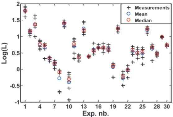
4.2. LİFESPAN _DİSTRİBUTİON

In a parametric AFT model, the distribution of lifespans under fixed conditions must be also verified. Fig. 2 shows the logarithms of the lifespans measured in minutes in each experiment.

1 4 7 10 13 16 19 22 25 28 30 -1 -0.5 0 0.5 1 1.5 2 Exp. nb. L o g (L ) Measurements Mean Median

Fig. 2. Lifespan data

Since only six lifespan measurements per experiment are available, it is difficult to assess wether the underlying distribution of Log(L) is a normal or an EV distribution. However, there are four central points (N0 = 4), with six lifespan

measurements for each. Therefore, 24 lifespans are measured under the same central conditions and compose a larger dataset to test the underlying distribution. Central point distribution is thus tested with three different methods: graphical tests, hypothesis tests, and distribution goodness of fit. Graphical tests [12] allow a first comparison between the empirical and theoretical normal or EV cumulative density function (cdf). Fig. 3 shows that the differences between empirical and theoretical cdf are higher in the case of EV distribution.

2.2 2.3 2.4 2.5 2.6 0 0.2 0.4 0.6 0.8 1 x Pf (x ) Empirical cdf Theoretical Normal cdf Difference 2.2 2.3 2.4 2.5 2.6 0 0.2 0.4 0.6 0.8 1 x Pf (x ) Empirical cdf Theoretical EV cdf Difference

Fig. 3. Graphical tests for normal (left) and extreme value (right) distributions applied to central points

These results can be confirmed with well-known hypothesis tests based on the difference between empirical and theoretical cdf [13],[14]: Kolmogorov-Smirnov, Lilliefors and Anderson-Darling tests. The null hypothesis of these tests is that the underlying distribution of the central point

Log(L) is the normal or the EV distribution. The

alternative hypothesis is that they are not. Table II summarizes the p-values of these tests in both cases. This table shows that normal distribution hypothesis is accepted with higher p-values, which confirms the graphical test results.

Table III. Results of hypothesis distribution tests applied to central points

Hypothesis test Normal

distribution EV distribution Kolmogorov-Smirnov 0.981 0.628 Lilliefors 0.888 0.167 Anderson-Darling 0.793 0.138

Finally, using Matlab distribution fitting tool, it is possible to compare the goodness of fit of the central points measured Log(L) to each of the two distributions by evaluating the log-likelihood of the normal and EV fitting. Table III summarizes the distribution fitting estimated parameters (location parameter µ and scale parameter s) and the corresponding log-likelihood in both cases.

Table IV. Results of distribution fitting applied to central points Distribution parameter Normal distribution EV distribution µ (std. error) 2.41 (0.018) 2.47 (0,018) s (std. error) 0.086 (0.013) 0.081 (0,012) Log-likelihood 25.3 23.9

The log-likelihood of normal fitting is higher than that of the EV fitting, which confirms that the normal distribution fits better the central point lifespans than EV distribution.

Under AFT model assumptions, stress factors only shift the location parameter of Log(L). Therefore, the same (normal) distribution can be assumed to

Log(L) measured under the other stress conditions,

in particular, those required to construct the lifespan model (8 blue points of Fig. 1). This hypothesis will be confirmed with different methods in section 5.

5. M

E

V

Equation (3) has the general form of a multi-linear regression model between Log(L) and the predictor variables (main factors and interaction terms). With the normality assumption verified with previous tests, model (3) coefficients can be estimated using the OLS method. They are shown in Fig. 4. Therefore, voltage and temperature have the highest main effects (EV and ET) and interaction (IVT).

-0.6 -0.5 -0.4 -0.3 -0.2 -0.1 0 0.1 EV EF ET IVF IVT IFT IVFT

Fig. 4. DoE model estimated coefficients In general, an AFT model having the general form of a multi-linear regression model as (3) must verify the following basic hypotheses [15],[16]:

1. Linearity of (Y,X) relationship 2. Full rank X

3. Non-stochastic X 4. n ³ p+1

5. Zero-mean residuals

6. Homoscedasticity (residual constant variance) 7. Residual normality

While hypotheses 2, 3 and 4 are naturally satisfied by model (3), it is important to perform a residual analysis in order to verify hypotheses 1, 5, 6 and 7.

5.1. RESİDUAL ANALYSİS

Residual graphical analysis is the most informative study that can be performed to check a multi-linear regression model assumptions [15],[16]. First, the scatterplot of residuals against the predicted values of Y allows to check hypotheses 1, 5 and 6. If these hypotheses are satisfied, then residuals will be randomly distributed around zero with no noticeable pattern of residual dependency on the predicted Y values. Second, residual normality (hypothesis 7) can be checked with QQ-plots (quantile-quantile plots). This graphical tool plots the observed residual quantiles against the corresponding theoretical normal quantiles. If residuals are normally distributed, the QQ-plot follows a straight line. Fig. 5 shows model (3) residual graphics. First, the scatterplot of Fig. 5 shows that residuals are randomly distributed around zero, except for only 4 points (8% of the total number of points). These are the same points that do not belong to the straight line formed by the other points of the QQ-plot. From these two

graphics, homoscedasticity and residual normality can be globally confirmed.

-0.5 0 0.5 1 1.5 2 -0.5 -0.3 -0.1 0.1 0.3 R e s id u a ls Y_predicted -2 -1 0 1 2 -0.5 -0.3 -0.1 0.1 0.3

Standard normal quantiles

R e s id u a l q u a n ti le s

Fig. 5. DoE model residual analysis Residual properties are directly related to the response form Y=Log(L). Therefore, homoscedasticity of model (3) can be also confirmed by testing other commonly used functions of the lifespan as the model response. Fig. 6 a to d show residual scatterplots of four models estimated as in (3) but with responses Y respectively equal to 1/L, 1/ÖL, L and ÖL, instead of

Log(L). 0 0.5 1 1.5 2 2.5 -3 -2 -1 0 1 2 3 R e s id u a ls Y_predicted Fig. 6.a. DoE model residual analysis with

Y=1/L 0 0.5 1 1.5 -0.8 -0.4 0 0.4 0.8 R e s id u a ls Y_predicted Fig. 6.b. DoE model residual analysis with

Y=1/ÖL 0 2 4 6 8 -2 -1 0 1 2 R e s id u a ls Y_predicted Fig. 6.c. DoE model residual analysis with

Y=ÖL 0 10 20 30 40 50 60 70 -20 -10 0 10 20 R e s id u a ls Y_predicted Fig. 6.d. DoE model residual analysis with

Y=L

These scatterplots show a special pattern of the residual variation with respect to predicted Y. In particular, residual values and dispersion increase as Y increases. Compared to these four functions, the logarithmic transformation is the most appropriate response form that can satisfy model basic hypotheses. Therefore, this result confirms the choice of Log(L) as model (3) response.

5.2. COEFFİCİENT _STATİSTİCAL _PROPERTİES

Under the residual normality assumption verified in the previous section, a statistical analysis can be performed on model (3) coefficients. İn particular, coefficient variability can be evaluated by computing the standard errors (SE) and their

confidence intervals (CI). The CI based on an OLS estimated coefficient bj (j = 1 ... p) for a confidence

level (1-a ) can be computed as [15],[16]:

)] 1 ( ) ( ˆ ); 1 ( ) ( ˆ [ ) ( 2 1 2 1 -+ -= -p n t SE p n t SE CI j j j j j a a b b b b b (4) where 1 ) ˆ ( )' ˆ ( ˆ ) ' ( ˆ ) ( 2 1 2 2 -= = -p n X Y X Y X X diag SE j b b s s b (5) and ( 1) 2 1 -- n p

t _a is the quantile of order (

2 1-a ) of the Student distribution having (n- p-1) degrees of freedom. Moreover, the statistical significance of each coefficient in the model can be assessed with the Student test (St. Test). The idea is to test whether the normalized value of an estimated coefficient bˆ_j/SE(b_j) is significantly different from zero. The rejection zone of this test is therefore [15],[16]: ) 1 ( ) ( ˆ 2 1 -³ - n p t SE _j j a b b (6) Table III shows the statistical properties of model (3) coefficients.

Table IV. DoE model coefficients and their statistical properties Coef. Estimated value 95% CI p-value (St. test) M 0,742 [0,692 ; 0,791] 0,000 EV -0,522 [-0,571 ; -0,472] 0,000 EF -0,236 [-0,286 ; -0,187] 0,000 ET -0,253 [-0,303 ; -0,204] 0,000 IVF -0,036 [-0,085 ; 0,014] 0,153 IVT 0,061 [0,012 ; 0,111] 0,016 IFT -0,010 [-0,059 ; 0,040] 0,697 IVFT -0,018 [-0,067 ; 0,032] 0,476

Therefore, we can confirm that the three factors and the most important interaction (VT) having the highest estimated effects (EV, EF, ET and IVT) are

statistically significant at 95% significance level.

5.3. NON-PARAMETRİC BOOTSTRAP METHOD

In this section, an alternative method to validate model (3) statistical properties is presented. With small size training sets as those involved in the DoE method, it might be difficult to assess some hypothesis regarding statistical properties. In the

previous section, a statistical analysis of the model coefficients based on residual normality assumption was performed. This hypothesis was verified through preliminary tests on central point distribution and with residual graphics. In this section, coefficient properties will be evaluated with the non-parametric bootstrap method. This method was introduced by Efron in 1979 [7] in order to derive statistical properties of an estimator based on a non-parametric resampling of the data. In regression problems, the idea is to obtain a high number B (50 < B < 200) of replications of model coefficients b* and to use these replications to

compute their statistical properties. Two resampling methods exist for regression models [8]:

1. Bootstrap on xy pairs: B models are estimated by making random sorts with retrieval of pairs (X*,Y*) in the original (X,Y) sample.

2. Bootstrap on residuals: B models are estimated by creating new response values Y* from random sorts with retrieval of residuals in the original residual sample.

Using the obtained bootstrap replications b*, their

standard errors SE(b), their confidence intervals CI(b) and their statistical significance (St. test

p-values) can be computed as shown in

Fig. 7 a and b [8],[9]. Since no assumption is made on the underlying distribution, the bootstrap method can be particularly interesting for making statistical inference on small size samples as in the case of DoE model training sets. The bootstrap method is applied on model (3) coefficients with B = 200 and using the two resampling methods.

Fig. 7.a. Bootstrap SE and CI

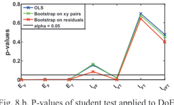
Fig. 8 a and b show respectively the coefficient CI and p-values of Student test obtained with the bootstrap method, as well as those computed under residual normality assumption (see Table IV).

-0.6 -0.4 -0.2 0 0.2 EV EF ET IVF IVT IFT IVFT

OLS estimated coef. CI (OLS)

CI (Bootstrap on xy pairs) CI (Bootstrap on residuals)

Fig. 8.a. Confidence Intervals for DoE model coefficients under residual normality assumption

and with bootstrap

0 0.2 0.4 0.6 0.8 p -v a lu e s EV EF ET IVF IVT IFT IVFT OLS Bootstrap on xy pairs Bootstrap on residuals alpha = 0.05

Fig. 8.b. P-values of student test applied to DoE model coefficients under residual normality

assumption and with the bootstrap method

6. C

_F

_W

This paper focussed on the parametric modelling of insulation lifespan in the very special case of a small number of training samples. Classical statistical methods such as graphical tools (Quantile-Quantile plots) and goodness-to-fit tests were implemented. However, to take into account the lack of data, the paper proposed a comparison with results obtained from a bootstrap procedure. The bootstrap method confirmed the underlying hypotheses we made for parameter estimation. The paper showed that the bootstrap technique is a powerful validation tool when the number of training samples is constrained.

REFERENCES

[1] L. Fang, I. Cotton, Z.J. Wang and R. Freer, “Insulation Performance Evaluation of High Temperature Wire Candidates for Aerospace Electrical Machine Winding”, in Proc. IEEE

Electrical Insulation Conf., 2013, pp. 253-256

[2] Y. Jinkyu, B. L. Sang, Y. Jiyoon, L. Sanghoon, O. Yongmin and C. Changho, “A Stator

Winding Insulation Condition Monitoring Technique for Inverter-Fed Machines”, IEEE Trans. on Power Electronics, vol. 22, no. 5, Sep. 2007

[3] L. Escobar and W. Meeker, “A review of accelerated test models”, Stat. Sci., vol. 21, no. 4, pp. 552-577, 2006.

[4] F. Salameh, A. Picot, M. Chabert, and P. Maussion, Regression methods for improved lifespan modelling of low voltage machine insulation, Math. Comput. Simul., vol. 131, pp. 200-216, 2017.

[5] F. Salameh, A. Picot, M. Chabert, E. Leconte, A. Ruiz-Gazen, P. Maussion, Variable importance assessment in lifespan models of insulating materials: a comparative study, 2015 IEEE Int. Symp. Diag. Electr. Mach. Power Electron. Drives (SDEMPED), pp. 198-204. [6] A. Picot, D. Malec, M. Chabert, P. Maussion,

Lifespan Modeling of Insulation Materials for Low Voltage Machines: films and twisted pairs. Symposium de Génie Electrique 2014, Cachan, France

[7] B. Efron, Bootstrap methods, another look at the jackknife, The Annals of Statistics, vol. 7, no. 1, pp. 1-26, 1979.

[8] B. Efron and R. J. Tibshirani, An introduction to the bootstrap, NY: Chapman and Hall, 1993. [9] J. G. Mackinnon, Bootstrap methods in econometrics, Economic Record, vol. 82, no. s1, pp. S2-S18, 2006.

[10] D. Collet, Modelling survival data in medical research, Chapman and Hall, London, 2003. [11] J. F. Lawless, Statistical models and methods

for lifetime data, Second edition, Wiley, 2003. [12] J. D. Jobson, Applied Multivariate Data

Analysis: Regression and Experimental Design, Springer, New York, 1999

[13] T. W. Anderson, D. A. Darling, A Test of Goodness-of-Fit, Journal of the American Statistical Association, vol. 49, no. 268, pp.765-769, 1954.

[14] H. Lilliefors, On the Kolmogorov–Smirnov test for normality with mean and variance unknown, Journal of the American Statistical Assoc, vol. 62, no. 318, pp. 399-402, 1967. [15] D. A. Freedman, Statistical models, theory and

practice, Cambridge university press, 2009. [16] S. Weisberg, Applied linear regression, Wiley,