This is an author-deposited version published in:
http://oatao.univ-toulouse.fr/
Eprints ID: 10684
To link to this article: DOI: 10.1007/s00498-014-0124-z
URL: http://dx.doi.org/10.1007/s00498-014-0124-z
To cite this version: Haine, Ghislain Recovering the observable part of the
initial data of an infinite-dimensional linear system with skew-adjoint
generator. (2014) Mathematics of Control, Signals, and Systems . ISSN
0932-4194
O
pen
A
rchive
T
oulouse
A
rchive
O
uverte (
OATAO
)
OATAO is an open access repository that collects the work of Toulouse researchers and
makes it freely available over the web where possible.
Any correspondence concerning this service should be sent to the repository
administrator: [email protected]
Recovering the observable part of the initial data
of an infinite-dimensional linear system
with skew-adjoint generator
Ghislain Haine
Abstract We consider the problem of recovering the initial data (or initial state) of
infinite-dimensional linear systems with unitary semigroups. It is well-known that this inverse problem is well posed if the system is exactly observable, but this assump-tion may be very restrictive in some applicaassump-tions. In this paper we are interested in systems which are not exactly observable, and in particular, where we cannot expect a full reconstruction. We propose to use the algorithm studied by Ramdani et al. in (Automatica 46:1616–1625, 2010) and prove that it always converges towards the observable part of the initial state. We give necessary and sufficient condition to have an exponential rate of convergence. Numerical simulations are presented to illustrate the theoretical results.
Keywords Linear systems · Inverse problems · Controllability · Observability · Feedback control
1 Introduction
1.1 Motivation
In many areas of science, we need to recover the initial (or final) data of a physical system from partial observation over some finite time interval. In oceanography and
G. Haine (
B
)ISAE, 31 055 Toulouse, France e-mail: [email protected] G. Haine
Université de Lorraine-CNRS, IECN, 54 506 Vandoeuvre-lès-Nancy, France G. Haine
meteorology, where this problem is known as data assimilation, we can mention the works of Auroux and Blum [1–3], Gejadze et al. [19,27], Shutyaev and Gejadze [34], Teng et al. [38] and the monograph of Blum et al. [7] concerning the numerical aspects. This problem also arises in medical imaging, for instance in thermoacoustic tomog-raphy. There, the problem is to recover the initial data of a wave type equation from surface measurements (see Gebauer and Scherzer [18] and the survey of Kuchment and Kunyansky [26]).
In the last decade, new algorithms based on time reversal (see Fink [15,16]) have been proposed for this problem. We can mention, for instance, the Back and Forth Nudging proposed by Auroux and Blum [1], the Time Reversal Focusing by Phung and Zhang [31], the algorithm proposed by Ito et al. [24] and finally, the one we will consider in this paper, the forward–backward observers-based algorithm proposed by Ramdani et al. [32] (which is a generalization of the one in [31]). In this paper, we study the convergence of the reconstruction algorithm of [32] for systems with skew-adjoint generator, when the inverse problem is ill-posed, that is to say when either the observability or the estimatability assumption fails.
To make this statement precise, let us begin with some notation and definitions. Let
X be a Hilbert space and A a skew-adjoint operator on X . We are interested in the reconstruction of the initial data z0of
!
˙z(t ) = Az(t )
z(0) = z0∈ X. ∀ t ≥ 0, (1.1)
Such equations are often used to model vibrating systems (acoustic or elastic waves) or quantum systems (Schrödinger equations).
By Stone’s Theorem (see for instance Tucsnak and Weiss [39]), A is the infinitesimal generator of a unitary C0-group S on X , and in particular, kz(t )k = kz0k for all t ≥ 0. Let Y be another Hilbert space. We suppose that we have access to z through the operator C : D( A) → Y , during a time interval [0, τ ], τ > 0, leading to the measurement
y(t ) = C z(t ) ∀ t ∈ [0, τ ]. (1.2) We call C the observation operator of the system. The observation is said to be bounded if C is a bounded operator (i.e. C ∈ L(X, Y )), and unbounded otherwise. In the latter case, we still assume that C is bounded with respect to the graph norm of A on D( A). For systems described by evolution partial differential equations (i.e. when A is a differential operator in the space variables on a domain Ω), bounded observation generally corresponds to measurement on a subdomain O ⊂ Ω, while unbounded observation in most cases corresponds to measurement on the boundary of Ω.
If we denote Ψτthe operator which associates the output function y|[0,τ ]to an initial data z0 ∈ D( A), the inverse problem is well posed when Ψτ is left-invertible, with bounded left-inverse. This is equivalent to Ψτ being bounded from below
∃kτ >0, kΨτz0k ≥ kτkz0k ∀ z0∈ D( A). (1.3)
Now, we present the algorithm proposed by Ramdani et al. [32]. For simplicity, we consider the particular case where A is skew-adjoint and C ∈ L(X, Y ), the pair (A, C)being exactly observable in time τ > 0. Let T+be the exponentially stable
C0-semigroup generated by A+ = A − γ C∗C, while T− is generated by A− = − A − γ C∗C, for some γ > 0 (see Liu [28]). For all n ∈ N∗, we define the following systems ˙z+ n(t ) = A+z+n(t ) + γ C∗y(t ) ∀ t ∈ [0, τ ], z+1(0) = z+0 ∈ X, z+n(0) = z−n−1(0) ∀ n ≥ 2, (1.4) & ˙zn−(t ) = − A−z−n(t ) − γ C∗y(t ) ∀ t ∈ [0, τ ], zn−(τ ) =z+n(τ ) ∀ n ≥ 1. (1.5)
The forward error en+(t ) = z+n(t ) − z(t )satisfies ˙en+(t ) = ( A − γ C∗C)e+n(t ) ∀ t ∈ [0, τ ], e1+(0) = z+0 − z0∈ X, en+(0) = e−n−1(0) ∀ n ≥ 2,
and the backward error en−(t ) = z−n(t ) − z(t ) & ˙e−n(t ) = ( A + γ C∗C)e−n(t ) ∀ t ∈ [0, τ ], e−n(τ ) =e+n(τ ) ∀ n ≥ 1. So, we have ' 'z− n(0) − z0 ' ' =''e− n(0) ' ' =''(T− τT + τ )n e+1(0)'' ≤''T−τT+ τ ' 'n''z+ 0 − z0 ' ' . (1.6) According to Ito et al. [24, Lemma 2.2], if ( A, C) is exactly observable in time τ , we have''T−τT+τ
'
'L(X )= α < 1 and thus
kz−n(0) − z0k ≤ αnkz+0 − z0k −→ n→∞0.
In the case of exactly observable systems, we call the systems (1.4)–(1.5) forward and backward observers as it is a generalization to infinite-dimensional systems of the so-called Luenberger’s observers [29], well-known in control theory. Observers for infinite-dimensional systems are an active topic of research, for both linear or non-linear systems, and among the large literature, we can cite for instance: Chapelle et al. [9], Krstic et al. [25], Moireau et al. [30], Smyshlyaev and Krstic [35], and Couchouron and Ligarius [10]. For pioneering work, we refer to Baras and Bensoussan [4] and Bensoussan [6].
In the paper of Ramdani et al. [32], they consider a wide class of infinite-dimensional systems (allowing even an observation operator that is not admissible). They suppose that the system is estimatable and backward estimatable (roughly speaking, the system can be forward and backward stabilized with a feedback operator called a stabilizing
output injection operator). However, they show in Proposition 3.3 that this implies that the system is exactly observable, or in other words, that (1.3) is satisfied (for some sufficiently large time τ ). In this paper, we are dealing with the initial data recovery of some well posed linear systems which are not supposed to be exactly observable, using the same algorithm.
By a well posed linear system we mean a linear time-invariant system Σ such that on any finite time interval [0, t], the operator Σt from the initial state z0and the input function u to the final state z(t ) and the output function y is bounded. In other words, Σis a family of bounded operators such that
* z(t ) y|[0,t] + = Σt * z0 u|[0,t] + .
Under some assumptions on the system Σ, we propose to investigate the above algo-rithm in the framework of well posed linear systems (allowing admissible observation operators) to recover the observable part of z0from y|[0,τ ]. The results on well posed linear systems used in this work will be recalled in Sect.2. For more details, we refer the reader, for instance, to the work of Salamon et al. [33,36,37,40–42] and the survey of Weiss et al. [45].
The paper is organized as follows. In Sect.2we give some background on well posed linear systems, including the construction of the dual system and the known results on colocated feedback. In Sect.3, we begin with the definition of two sys-tems, Σ+and Σ−, corresponding to the forward (1.4) and backward (1.5) observers, respectively. We then work on the properties of the operator T−τT+
τ, called the forward–
backward operator, which appears naturally. The properties of this operator, given in Proposition3.9, are needed to prove the main result of this paper. Finally, we prove the main result of this work, Theorem1.1, which shows that the algorithm leads to the reconstruction of the observable part of the initial state. In Sect.4, we apply our theoretical result to an N -dimensional (N ≥ 2) wave equation, with Dirichlet control and colocated observation on a part of the boundary.
1.2 Main results
From a well posed linear system Σ = *
T Φ Ψ F
+
, defined in Definition2.1and verifying some assumptions (namely A∗= − A and B = C∗), we will construct two other well posed linear systems Σ+and Σ−, corresponding to (1.4) and (1.5), respectively. All the needed terminology and results on well posed linear systems are recalled in Sect.2. Let us begin with the definition of the time-reflection operator. Let W be a Hilbert space. For all τ ≥ 0, we define the linear operator R τ : L2ℓoc([0, ∞), W ) →
( R τu) (t ) = !
u(τ − t ) ∀ t ∈ [0, τ ], 0 ∀ t > τ.
To state our main result, we need the operator Φτddefined in Theorem2.13. In the following theorem, we only need that Φτd = Ψτ∗ R τ, so that VObs = Ran Φτd can be understood as (Ker Ψτ)⊥. From that, the link with the known results in the case of exact observability (1.3) is obvious.
Theorem 1.1 Let X and Y be Hilbert spaces. Assume that Σ is a well posed linear
system with input and output space Y and state space X determined by the operators
(A, B, C) and the transfer function G, such that A∗ = − A and B = C∗. Using Theorems2.13and2.17, let us denote by Σ+(resp. Σ−) the closed-loop system of Σ (resp. Σd) with output feedback operator γ I , where γ ∈ (0, κ), for some κ ∈ (0, ∞]
(explicitly given in Remark2.18).
Let z0∈ X and denote u, z and y the input, trajectory and output of Σ, respectively,
with initial state z0. Let τ > 0, z+0 ∈ X and denote, for all n ≥ 1, z+n and z−n the
respective trajectories of Σ+ and Σ− with respective inputs v+ = γ y + u and v−= γ R τ y+ R τu, and initial states
z+1(0) = z+0 ∈ X, z+n(0) = zn−1− (0), n ≥ 2, z−n(τ ) =z+n(τ ), n ≥1.
Furthermore, we denote by Π the orthogonal projector from X onto VObs= Ran Φτd,
then the following statements hold true: 1. We have for all z0,z+0 ∈ X
'
'(I − Π)(z−n(0) − z0)''= '
'(I − Π)(z+0 − z0)'' ∀ n ≥ 1.
2. The sequence(''Π(z−n(0) − z0)'')n≥1is strictly decreasing and satisfies '
'Π(z−n(0) − z0)'' −→ n→∞0.
3. The rate of convergence is exponential,i.e. there exists a constant α ∈ (0, 1), independent of z0and z0+, such that
'
'Π(z−n(0) − z0)''≤ αn '
'Π(z+0 − z0)'' ∀ n ≥ 1, if and only if Ran Φτdis closed in X .
Theorem1.1allows us to approximate the projection of z0on VObsby the projection of z−n(0). However, in practice, it is difficult to characterize VObsand thus the projector Π. The following corollary shows that if the (arbitrary) initial guess z+0 belongs to
VObs (for example, one can take z+0 = 0), then all successive approximations z−n(0) belong to VObs, so that we do not need to know Π anymore.
Corollary 1.2 Under the assumptions of Theorem1.1, if z+0 ∈ VObs, then ' 'z− n(0) − Π z0 ' ' −→ n→∞0.
Furthermore, the decay rate is exponential if and only ifRan Φτdis closed in X .
We will prove this corollary in Sect.3.4.
2 Background on well posed linear systems
In this section, we recall some definitions used in the framework of well posed linear
systems, also called abstract linear systems. All this material can be found, for instance, in [33,36,37,40–42,45].
2.1 Definitions and associated operators A, B and C
We first define the τ -concatenation. For any τ ≥ 0 and any Z , Hilbert space, we define for all u, v in L2([0, ∞), Z ) the following binary operator
(u ⋄τ v) (t ) = !
u(t ) ∀ t ∈ [0, τ ), v(t − τ ) ∀ t ≥ τ.
Definition 2.1 (Well posed linear system) Let X , U and Y be Hilbert spaces. We
denote by U = L2([0, ∞), U ) and Y = L2([0, ∞), Y ). A well posed linear system on (U , X, Y) is a family of bounded operators Σ = (Σt)t ≥0from X × U to X × Y, where Σt = ,T t Φt Ψt Ft -, satisfying: – T = (Tt)t ≥0is a C0-semigroup on X ,
– Φ = (Φt)t ≥0is a family of bounded linear operators from U to X such that Φτ +t(u ⋄τ v) = TtΦτu + Φtv ∀u, v ∈ U , τ, t ≥0, – Ψ = (Ψt)t ≥0is a family of bounded linear operators from X to Y such that
Ψτ +tz = Ψτz ⋄τΨtTτz ∀ z ∈ X, τ, t ≥0, and Ψ0≡ 0,
– F = (Ft)t ≥0is a family of bounded linear operators from U to Y such that Fτ +t(u ⋄τv) = (Fτu) ⋄τ(ΨtΦτu + Ftv) ∀ u, v ∈ U , τ, t ≥ 0, and F0≡ 0.
We call U the input space of Σ, X the state space of Σ, and Y the output space of Σ. The operator Φτis called an input map, Ψτ an output map and Fτan input–output
Denoting by Pτ the projection of L2([0, ∞), Z ) on L2([0, τ ), Z ) (by truncation), one can easily show that ΦτPτ = Φτ, FτPτ = Fτ, PtΨτ = Ψt and PtFτPt =
PtFτ = Ft for all 0 ≤ t ≤ τ .
To be able to define the output y of the system Σ from its operators, we first need to define Ψ∞= lim τ →∞Ψτ ∈ L(X, Yℓoc), and F∞= lim τ →∞
Fτ ∈ L(Uℓoc, Yℓoc),
where Uℓoc and Yℓocare the Fréchet spaces defined by Uℓoc = L2ℓoc([0, ∞), U ) and Yℓoc = L2ℓoc([0, ∞), Y ) with the seminorms being the norms of Pτu, where τ > 0. Then, one can easily show that
Ψτ = PτΨ∞, Fτ = PτF∞.
We call Ψ∞an extended output map of Σ, and F∞an extended input–output map of Σ.
Definition 2.2 Let z0∈ X and u ∈ Uℓoc, the state trajectory z and the output function
yof Σ corresponding to the initial state z0and the input function u are defined by
z(t ) = Ttz0+ Φtu ∀ t ≥0,
y = Ψ∞z0+ F∞u. (2.1) One can easily see that
* z (t ) Pt y + = Σt * z0 Pt u + .
Let A be the infinitesimal generator of T, and ω0(T)its growth bound. We denote by X1the domain D( A) endowed with the graph norm, denoting by k · k1, and X−1the closure of X with the norm kzk−1= k(β I − A)−1zk(for some arbitrary β ∈ ρ( A), the resolvent set of A). It is well-known (see for instance Tucsnak and Weiss [39]) that these spaces are Hilbert spaces and that
X1⊂ X ⊂ X−1,
each inclusion being dense and with continuous embedding.
For any Hilbert space W , any interval J and any ω ∈ R, we denote by
L2ω(J, W ) = eωL2(J, W ), where (eωv)(t ) = eωtv(t ), with the norm keωvkL2
Proposition 2.3 There exists a unique operator B ∈ L(U, X−1), called the control
operator of Σ , such that for any initial state z0∈ X and any input function u ∈ Uℓoc,
the state trajectory z defined in(2.1) is the unique strong solution in X−1of !
˙z(t ) = Az(t ) + Bu(t ) ∀ t ≥ 0,
z(0) = z0.
Moreover, we know that z ∈ C([0, ∞), X ) ∩ Hℓoc1 ([0, ∞), X−1), and if u ∈
L2ω([0, ∞), U ) with ω > ω0(T), then z also belongs to L2ω([0, ∞), X ) and its Laplace
transform is
.z(s) = (s I − A)−1[z0+ B.u(s)] ∀ s ∈ Cω.
We can also prove that
Ψ∞∈ L(X, L2ω([0, ∞), Y )), and F∞∈ L/L2 ω([0, ∞), U ), L2ω([0, ∞), Y ) 0 . This enables us to represent y via its Laplace transform.
Proposition 2.4 There exist an analytic L(U, Y )-valued function G on Cω0(T), called the transfer function of Σ , and a unique operator C ∈ L(X1,Y ), called the observation
operator of Σ , with the following properties:
– For every z0 ∈ X and u ∈ L2ω([0, ∞), U ) with ω > ω0(T), the corresponding
output function y = Ψ∞z0+ F∞u belongs to L2ω([0, ∞), Y ) and its Laplace
transform is
.y(s) = C(s I − A)−1z0+ G(s).u(s) ∀ s ∈ Cω. (2.2)
– G satisfies for all α, β ∈ Cω0(T) G(α) − G(β)
α − β = −C(α I − A)
−1(βI − A)−1B,
(2.3)
or equivalently G′(α) = −C(α I − A)−2B. – G is bounded on Cω for every ω > ω0(T).
Note that according to the second statement, G is determined by A, B and C up to an additive constant.
For any C ∈ L(X1,Y ), we define its Λ-extension CΛby
CΛz0= lim
λ→∞Cλ(λI − A) −1z
0.
We denote D(CΛ)its domain, consisting of all z0 ∈ X for which the above limit exists. Then we have the following result (see Theorem3.2of [33] and [36])
Proposition 2.5 With the previous notation, if u ∈ Uℓoc, and z0∈ X , then for almost every t ≥0 y(t ) = CΛ , z(t ) − (β I − A)−1Bu(t )-+ G(β)u(t ) ∀ β ∈ Cω0(T). Furthermore, if u ∈ H0,ℓoc1 ([0, ∞), U ), y(t ) = CΛTtz0+ C , Φtu − (β I − A)−1Bu(t ) -+ G(β)u(t ) ∀ β ∈ Cω0(T). (2.4)
Curtain and Weiss [12] have given necessary and sufficient conditions for a triple of operators ( A, B, C) to be well posed (i.e. to be associated with a well posed lin-ear system Σ). We need the definition of admissibility for control and observation operators before stating the theorem.
Definition 2.6 Let X , U and Y be Hilbert spaces. Let A be the generator of a C0 -semigroup T on X , B ∈ L(U, X−1)a control operator and C ∈ L(X1,Y )an obser-vation operator.
– B is an admissible control operator for T if and only if for some (and hence any) τ >0, the operator Φτ, defined by
Φτu = τ 1 0
Tτ −sBu(s)ds ∀ u ∈ Uℓoc,
has its range in X .
– C is an admissible observation operator for T if and only if for some (and hence any) τ > 0, the operator Ψτdefined by
(Ψτz0) (t ) = !
CTtz0 ∀ t ∈ [0, τ ]
0 ∀ t > τ ∀ z0∈ X1, has a continuous extension to X .
Remark 2.7 It is clear that C is an admissible observation operator for T if and only if C∗is an admissible control operator for T∗.
Theorem 2.8 (Generating triple, Theorem 5.1 of [11]) Let X , U and Y be three Hilbert
spaces.
A triple of operators ( A, B, C) is well posed (i.e. associated with a well posed linear system Σ) if:
1. A is the generator of a C0-semigroup T on X ,
2. B ∈ L(U, X−1)is an admissible control operator for T, 3. C ∈ L(X1,Y )is an admissible observation operator for T,
4. there is an α ∈ R such that some (and hence any) solution G : ρ( A) → L(U, Y ) of the equation (2.3) is bounded on Cα(i.e. G is proper).
Conversely, if Σ is a well posed linear system, with associated triple of operators (A, B, C)and the transfer function G, then the four previous conditions are satisfied.
2.2 Optimizability, estimatability, controllability and observability
It is well-known that for any C0-semigroup T, we have the following property: ∀ω > ω0(T), ∃Mω≥ 1 : kTtz0k ≤ Mωeωtkz0k ∀ z0∈ X.
If we have ω0(T) < 0, then there is ω < 0 satisfying this inequality and the C0 -semigroup will decay exponentially in time. This justifies the following definition.
Definition 2.9 A well posed linear system Σ is exponentially stable if and only if
ω0(T) <0.
Let us recall some definitions, which can be found in Weiss and Rebarber [44].
Definition 2.10 Let X , U and Y be Hilbert spaces. Let A be the generator of a C0 -semigroup T on X , B ∈ L(U, X−1)an admissible control operator for T and C ∈ L(X1,Y )an admissible observation operator for T.
– The pair ( A, B) is optimizable if for every z0∈ X , there exists a u ∈ U such that
z ∈ L2([0, ∞), X ), where z(t ) = Ttz0+ t 1 0 Tt −sBu(s)ds.
– The pair ( A, C) is estimatable if ( A∗,C∗)is optimizable.
A well posed linear system Σ is said to be optimizable if its corresponding pair ( A, B) is optimizable, and estimatable when its corresponding pair ( A, C) is estimatable.
Definition 2.11 Let X , U and Y be Hilbert spaces. Let A be the generator of a C0 -semigroup T on X , B ∈ L(U, X−1)an admissible control operator for T and C ∈ L(X1,Y )an admissible observation operator for T.
– The pair ( A, B) is exactly controllable in time τ > 0 if Ran Φτ = X . It is
approximately controllablein time τ > 0 if Ran Φτ = X .
– The pair ( A, C) is exactly observable in time τ > 0 if there exists a constant
kτ >0 such that
kΨτz0k ≥ kτkz0k ∀ z0∈ X. It is approximately observable in time τ > 0 if Ker Ψτ = {0}.
Remark 2.12 The pair ( A, C) is exactly observable (approximately observable) if and only if ( A∗,C∗)is exactly controllable (approximately controllable).
2.3 The dual system
We introduce now the dual system of a well posed linear system.
Theorem 2.13 (Theorem 4 of [45] ) Let Σ = *
T Φ Ψ F
+
be a well posed linear system with input space U , state space X and output space Y . Define Σd=(Σtd)t ≥0by
Σtd= * Td t Φtd Ψtd Fd t + = * I 0 0 R t + * T∗ t Ψt∗ Φt∗ F∗t + * I 0 0 R t + . (2.5) Then, Σd= * Td Φd Ψd Fd +
is a well posed linear system with input space Y , state space X and output space U . In particular, ω0(T) = ω0(Td). The linear system Σdis called
the dual system of Σ .
Proposition 2.14 (Proposition 4 of [45]) If A, B and C are respectively the semigroup
generator, control operator and observation operator of the well posed linear system
Σ with growth bound ω0(T), then the corresponding operators for Σd are A∗, C∗
and B∗. The transfer functions are related by
Gd(s) = G∗(s) ∀ s ∈ Cω0(T).
2.4 Feedback law
The results of this subsection allow us to construct the forward and backward observers in the framework of well posed linear systems.
Definition 2.15 Let Σ be a well posed linear system with input space U , state space
X, output space Y and transfer function G. An operator K ∈ L(Y, U ) is called an
admissible feedback operatorfor Σ if I − GK has a well posed inverse on some right half-plane (equivalently, if I − K G has a well posed inverse).
Theorem 2.16 (Theorem 6.1 of [41]) If K is an admissible feedback operator for
a well posed linear system Σ , the closed-loop system ΣK,i.e. Σ with the output feedback u = K y + v (v is the new control), is well posed. Furthermore, we have
ΣK− Σ = Σ * 0 0 0 K + ΣK = ΣK * 0 0 0 K + Σ. (2.6)
Under some assumptions, Curtain and Weiss [12, Theorem 5.8] proved that the colocated feedback law exponentially stabilizes the well posed linear system. This generalizes, in some sense, the known results when A is skew-adjoint and C is bounded (see Liu [28]). We give a simpler version of this result, in our particular case.
Theorem 2.17 Suppose that Σ is a well posed linear system such that A is
skew-adjoint, U = Y and B = C∗. Then, there exists a κ > 0 (possibly κ = +∞) such
that for all γ ∈ (0, κ), the feedback law −γ y + v (v is the new control) leads to a
closed-loop system Σγ which is well posed.
Moreover, if Σ is optimizable and estimatable, then the closed-loop system Σγ is exponentially stable.
Remark 2.18 The value of κ is explicitly given in [12, Theorem 5.8]. We have κ = kE+k−1, where E+is the positive part of the self-adjoint operator
E = −1
2 2
G∗(λ) + G(λ)3+ λC (λI + A)−1(λI − A)−1C∗ ∀ λ > 0. (2.7)
Furthermore, if 0 ∈ ρ( A), then
E = −1
2 2
G∗(0) + G(0)3.
3 Algorithm of reconstruction
From now on, we suppose that Σ = *
T Φ Ψ F
+
is a well posed linear system with input space U , state space X , output space Y , determined by the operators ( A, B, C) and the transfer function G, such that
1. A is skew-adjoint, 2. U = Y and B = C∗.
Note that from Stone’s Theorem, A is the generator of a unitary C0-group, which will be denoted by S. In the sequel, we suppose without loss of generality that the control
uof Σ satisfies u ≡ 0.
3.1 The forward and backward observers
Let us begin with a forward observer Σ+ of Σ (corresponding to (1.4)). With the above assumptions, we apply Theorem2.17to define the closed-loop system Σ+for some γ ∈ (0, κ).
In the first section of this paper, we have seen that the forward error e+(t ) = z+(t ) − z(t )satisfies ˙e+= ( A − γ C∗C) e+by simple algebraic computations. Here,
A − γ C∗Chas no more meaning, since C is unbounded. Therefore, we use directly the definitions of the trajectories z and z+to show that e+(t ) = T+t e(0).
We denote by *
T+ Φ+ Ψ+F+
+
the operators of Σ+. Then from (2.6) with K = −γ I , we have T+t z0+= Stz+0 − γ ΦtΨt+z+0 = Stz+0 − γ Φ + t Ψtz+0 ∀ z + 0 ∈ X. (3.1)
Let us denote by z and z0, respectively by z+and z+0, the trajectory and initial state of Σ, respectively Σ+. We add the control v = γ y to Σ+, where y is the output function of the initial system Σ. Note that y = Ψ∞z0since we suppose that u ≡ 0 (see (2.1) in Definition2.2). We have z(t ) = Stz0, z+(t ) = T+t z + 0 + γ Φ + t y ∀ z0,z+0 ∈ X.
From the above equalities and Φt+y = Φt+Pty = Φt+PtΨ∞z0 = Φt+Ψtz0, we can rewrite
z+(t ) = Stz+0 − γ Φt+Ψt(z+0 − z0) ∀ z0,z0+∈ X.
Then, we call Σ+a forward observer of Σ, since under some additional assumptions,
z+(t ) → z(t )as t → ∞. Indeed, e+(t ) = z+(t ) − z(t )satisfies e+(t ) = St ( z+0 − z0 ) − γ Φt+Ψt ( z+0 − z0 ) = T+t (z+0 − z0 ) ∀ z0,z+0 ∈ X,
and following Theorem2.17, T+is exponentially stable if (and only if) Σ is optimiz-able and estimatoptimiz-able.
Now, the idea is to go back in time, starting from z−τ = T+τz +
0 for a fixed finite time τ > 0. Thus, we have to define a backward observer Σ−of Σ (corresponding to (1.5)). We first define Σd =
* Td Φd Ψd Fd
+
, the dual system of Σ, using Theorem2.13. From Proposition 2.14, the C0-semigroup generator of Σd is A∗ = − A, and then the C0-semigroup of Σdis S−1= (S−t)t ≥0. From our assumptions, the control and observation operators of Σdare the same as those of Σ.
Before the definition of Σ−, we give the following lemma, immediate from (2.7), which shows that the same parameter γ can be used for both Σ+and Σ−.
Lemma 3.1 Let Σ be a well posed linear system verifying the assumptions of the
beginning of this section, and Σd its dual system. Denote κ and κd the maximal bound for γ in Theorem2.17, for Σ and Σd, respectively. Then κ = κd.
From now on, we take the same parameter γ ∈ (0, κ) for both Σ+and Σ−. We define by Σ−the closed-loop system of Σd, for some γ ∈ (0, κ). We denote by
*
T− Φ− Ψ−F−
+
the operators of Σ−. Then from (2.6) with K = −γ I , we have
T− t z − τ = S−tzτ−− γ Φ d tΨ − t z − τ = S−tz−τ − γ Φ − t Ψ d t z − τ ∀ z − τ ∈ X. (3.2) Denote by z−the trajectory of Σ−with the control v = γ R τ y. We know that Φτ− R τ
y = Φτ− R τΨτz0and it is easy to see that R τ Ψτ = ΨτdSτ, for all τ ≥ 0. Then, we get
z−(τ ) = S−τz−τ − γ Φτ−Ψτd (
Setting e−(t ) =( R τz− ) (t ) − z(t ), we obtain e−(0) = z−(τ ) −z0 = S−τzτ−− γ Φτ−Ψτd ( z−τ − Sτz0 ) − S−τSτz0 = S−τ ( z−τ − Sτz0 ) − γ Φτ−Ψτd(z−τ − Sτz0 ) = T−τ (z−τ − z(τ )).
And since z−τ = z+(τ ) = T+τz0+, we finally obtain
e−(0) = T−τT+ τ ( z0+− z0 ) .
If Σ is optimizable and estimatable, then there exists a τ > 0 such that kT−
τT+τkL(X ) <1 (since T+and T−are then exponentially stable). In other words,
z−(0) is a better approximation of z0than z+0. The iteration of this process gives a method to reconstruct z0with exponential decay of the error, as after n iterations we have ke−n(0)k ≤ ' 'T− τT+τ ' 'n L(X ) ' 'z+ 0 − z0 ' ' ∀ n ∈ N.
3.2 Relation between Σ+and Σ−
In this subsection we prove the following theorem, which will be useful in many computations.
Theorem 3.2 With the assumptions given at the beginning of this section, we have
(
Σ+)d= Σ−.
The proof of this result is based on the following equalities.
Lemma 3.3 With the assumptions and notation of Theorem3.2, we have
(I + γ Fτ)−1Ψτ = R τ(I + γ R τFτ R τ)−1 R τΨτ, (3.3) Fτ(I + γ Fτ)−1= Fτ R τ(I + γ R τFτ R τ)−1 R τ. (3.4)
Proof Remark that from (2.6), (I + γ Fτ)
(
I − γ F+τ)= I =(I − γ F+τ)(I + γ Fτ), showing that (I + γ Fτ)−1= I − γ F+τ.
On the other hand, we easily obtain that ( I − γ R τF+τ R τ ) (I + γ R τFτ R τ) = I + γ R τ ( Fτ − F+τ − γ F+τFτ) 4 56 7 =0 from (2.6) R τ = (I + γ R τFτ R τ) ( I − γ R τF+τ R τ ) .
In other words, (I + γ R τFτ R τ)−1 = I − γ R τF+τ R τ; hence, we have to prove that equality (3.3) reduces to ( I − γ F+τ)Ψτ = R τ ( I − γ R τF+τ R τ ) R τΨτ. But R τ ( I − γ R τF+τ R τ ) R τΨτ = PτΨτ − γ PτF+τPτΨτ = Ψτ− γ F+τΨτ = ( I − γ F+τ)Ψτ.
Similarly, equality (3.4) reduces to Fτ(I − γ F+τ)= Fτ R τ ( I − γ R τF+τ R τ ) R τ, and Fτ R τ(I − γ R τF+τ R τ ) R τ = FτPτ− γ FτPτF+τPτ = Fτ− γ FτF+τ = Fτ ( I − γ F+τ). ⊓ ⊔
Proof (Proof of Theorem3.2) We have to show that ( T+ τ )d = T−τ, (Φτ+)d = Φτ−, (Ψτ+)d= Ψτ−, (F+ τ )d = F−τ.
Let us begin with(Φτ+)d= Φτ−. Using τ∗R = R τ, (2.5), (2.6) and (3.3), we have ( Φτ+)d =(Ψτ+)∗ R τ = Ψτ∗ R τ ( I + γ R τF∗τ R τ )−1 R τ R τ = Φd τ ( I + γ Fdτ)−1Pτ = Φτ−.
Similarly, we obtain(Ψτ+)d = Ψτ−. Then, using (3.2), we have(T+ τ )d = (T+ τ )∗ = S−τ − γ Φτ−Ψτd = T−τ.
It remains to show that(F+τ)d = F−τ. Again, from τ∗R = R τ, (2.5), (2.6) and (3.4), we have ( F+ τ )d = R τ ( F+ τ )∗ R τ = R τ R τ ( I + γ R τF∗τ R τ )−1 R τF∗τ R τ = F−τ. ⊓ ⊔
3.3 The forward–backward operator
We now study in the general case the forward–backward operator T−τT+τ, for a fixed τ, with γ ∈ (0, κ). In other words, we suppose neither that Σ is optimizable and estimatable, nor that τ is large enough to ensure that kT−τT+τkL(X )<1.
Let us introduce the following orthogonal decomposition of an element z of X .
Lemma 3.4 With the previous notation and definitions, we have
X =Ker Ψτ⊕ Ran Φτd.
Proof This follows immediately from the decomposition X = Ker Ψτ⊕ (Ker Ψτ)⊥= Ker Ψτ⊕ Ran Ψτ∗and from Φτd= Ψτ∗ R τ(see Eq. (2.5)), since, obviously, Ran Ψτ∗= Ran2Ψτ∗ R τ
3
. ⊓⊔
In the sequel of the paper, we denote by VObs = Ran Φτd and VUnobs = Ker Ψτ, which correspond respectively to the observable part and to the unobservable part of an element of X . Proposition 3.5 We have ( T− τT + τ ) VObs⊂ VObs, ( T− τT + τ ) VUnobs⊂ VUnobs.
Proof From (3.1) and (3.2), we have T−
τT+τ = I − γ S−τΦτΨτ+− γ Φτ−ΨτdSτ + γ2Φτ−ΨτdΦτΨτ+. (3.5) First, note that from (2.5)
S−τΦτ = Φd
τ R τ = Ψτ∗Pτ.
Second, simple computations give ΨτdSτ = R τΨτand Theorem3.2shows that Φ− τ = (
Ψτ+)∗. Finally, from (2.6), we see that
Ψτ+= (I + γ Fτ)−1Ψτ, and then (3.5) becomes
T−τT+τ = I − γ Ψτ∗(I + γ Fτ)−1Ψτ− γ Ψτ∗ ( I + γ F∗τ)−1 R τΨτ +γ2Ψτ∗(I + γ F∗τ)−1 τR ΨτdΦτ(I + γ Fτ)−1Ψτ. Thus, by Lemma3.4 8 T− τT + τz, θ 9 = hz, θ i = 0, 8T− τT + τθ,z 9 = hθ, zi = 0 ∀ z ∈ VObs, θ ∈VUnobs, and then T−τT+τ )
VObs⊂ VObsand(T−τT+τ )
Remark 3.6 We point out the fact that kT−τT+τzk = kzkfor all z ∈ VUnobs. We immediately obtain the following result
Corollary 3.7 Let Π be the orthogonal projector from X onto VObs, then T−
τT+τΠ = Π T−τT+τ.
Proposition 3.8 Denote by L =(T− τT+τ
)
|VObs ∈ L(VObs). Then L is a positive
self-adjoint operator on VObs.
Proof From Theorem3.2, we have for all z1,z2∈ X 8T− τT+τz1,z29=8T+τz1, T+τz29. Then 8 T− τT + τz, z 9 =''T+τz''2 ∀ z ∈ X. (3.6) Thus T−τT+τ is positive self-adjoint on X , and a fortiori L is positive self-adjoint on
VObs(by Proposition3.5). ⊓⊔
Proposition 3.9 Let L be as in Proposition3.8. Then the following statements hold: 1. For all z ∈ VObs\{0}, we have kL zk < kzk.
2. We have the following characterization
kLkL(VObs)<1 ⇐⇒ VObs= Ran Φ
d
τ = Ran Φ d τ. We need two lemmas to prove this proposition.
Lemma 3.10 Let Σ =,T Φ
Ψ F
-be a well posed linear system satisfying the assump-tions of the beginning of this section. We have for all u ∈ Uℓoc
(
Φτ∗Φτ− F∗τ− Fτ )
u(t ) =2Eu(t ) for a.e. t ∈ (0, τ ),
where E is the self-adjoint operator defined by(2.7).
Proof Let Σd= *
Td Φd Ψd Fd +
be the dual system of Σ. We first remark that Φτ∗Φτ− F∗τ = R τΨτdΦτ− R τFdτ R τ.
Let u be a control belonging to
Hτ = {w ∈ Hℓoc1 ([0, ∞), Y ) | w(0) = w(τ ) = 0},
and z the trajectory of Σ with null initial state and control u. Then, z satisfies !
˙z(t ) = Az(t ) + C∗u(t ) ∀ t ∈ [0, τ ],
z(0) = 0,
Now, we consider zd(t ) = R τ z(t ) = z(τ − t ). Then, zd(t )is the trajectory of Σd with control v = − R τuand initial state Φτu
!
˙zd(t ) = − Azd(t ) − C∗ R τu(t ) ∀ t ∈ [0, τ ],
zd(0) = Φτu.
The output of Σdis then yd= ΨτdΦτu − Fdτ R τ u. Now, we have that
R
τyd− y = R τΨτdΦτu − R τFdτ R τu − Fτu.
Since u ∈ Hτ, we have in particular that u and R τ ubelong to H0,ℓoc1 ([0, ∞), Y ) and from (2.4), with β = λ > 0, we have for almost every t ∈ (0, τ )
R τyd(t ) − y(t ) = R τCΛdS−tΦτu + R τC , Φtdu + (λI + A)−1C∗ R τu(t ) -−C,Φtu − (λI − A)−1C∗u(t ) -− (G∗(λ) + G(λ))u(t ).
But CΛd is an extension of C, thus we can rewrite the above equality
R
τyd(t ) − y(t ) = CΛd
2
R
τzd(t )+(λI + A)−1C∗ R 2τu(t )
− z(t)+(λI − A)−1C∗u(t )3−(G∗(λ)+G(λ))u(t ) for a.e. t ∈ (0,τ ),
Since zd(t ) = R τ z(t )and R 2τ u(t ) = u(t )on (0, τ ), this becomes
R
τyd(t ) − y(t ) = CΛd 2
(λI + A)−1+ (λI − A)−13C∗u(t )
−(G∗(λ) + G(λ))u(t ) for a.e. t ∈ (0, τ ),
Now, using (λI − A)−1= − (−λI + A)−1for all λ > 0 and the resolvent identity, we get
R
τyd(t ) − y(t ) =2λCdΛ(λI + A)−1(λI − A)−1C∗u(t ) −(G∗(λ) + G(λ))u(t ) for a.e. t ∈ (0, τ ),
But (λI + A)−1(λI − A)−1C∗∈ L(Y, X1), and thus we can replace CΛd by C in the above equality, and (2.7) gives the result
R
τyd(t ) − y(t ) =2Eu(t ) for a.e. t ∈ (0, τ ),
We conclude by the density of Hτ in Uℓoc. ⊓⊔
Finally, we recall how to characterize the closure of the range of a bounded linear operator. We give this lemma without proof (see for instance Brézis [8, Chapter 2]).
Lemma 3.11 A bounded linear operator T ∈ L(Z1,Z2), where Z1and Z2are Hilbert
spaces, has a closed range if and only if there exists a constant k >0 such that kT∗f k ≥ kk(I − P) f k ∀ f ∈ Z2, (3.7)
where P is the orthogonal projector onKer T∗.
We are now able to prove Proposition3.9.
Proof (Proof of Proposition3.9) The two points of Proposition3.9are consequences of the following relation
kT+τzk2= kzk2− 2γ kΨτ+zk2+ 2γ2 8
E Ψτ+z, Ψτ+z9 ∀ z ∈ X, (3.8) where E is the self-adjoint operator of Remark2.18.
Let us begin with the proof of (3.8). kT+τzk2= kSτz − γ ΦτΨτ+zk2
= kSτzk2− γ hΦτ∗Sτz, Ψτ+zi − γ hΨτ+z, Φτ∗Sτzi + γ2kΦτΨτ+zk2.
From kSτzk = kzk, Φτ∗Sτ = Ψτ and Ψτ = (I + γ Fτ) Ψτ+, we obtain
kT+τzk2= kzk2−γh(I +γ Fτ) Ψτ+z,Ψτ+zi−γhΨτ+z, (I +γ Fτ) Ψτ+zi+γ2kΦτΨτ+zk2 = kzk2− 2γ kΨτ+zk2+ γ28(Φτ∗Φτ− Fτ− F∗τ
)
Ψτ+z, Ψτ+z9. We use now Lemma3.10to get (3.8).
We denote E+the positive part of E, then
kT+τzk2= kzk2− 2γ kΨτ+zk2+ 2γ28E Ψτ+z, Ψτ+z9 ≤ kzk2− 2γ kΨ+ τ zk2+ 2γ2kE4 56 7+k =κ−1 kΨ+ τ zk2 ≤ kzk2− 2γ(1 − γ κ−1)kΨ+ τ zk2.
where κ is the maximum bound for γ , given in Remark2.18. In particular we have 1 − γ κ−1>0. From this, if z ∈ VObs\{0}, thus kΨτ+zk2>0, and therefore
kL zk2= hL z, L zi =:L (L)12z, (L) 1 2 z ; = kT+τ (L)12 zk2 ≤ k (L)12 zk2− 2γ(1 − γ κ−1)kΨ+ τ (L) 1 2 zk2 ≤ hL z, zi ≤ kT+τzk2 ≤ kzk2− 2γ(1 − γ κ−1)kΨ+ τ zk2 < kzk2.
For the second point, we use the fact (from Ψτ = (I + γ Fτ) Ψτ+ and Ψτ+ = (
I − γ F+τ)Ψτ) that there exist two constants m, M > 0 such that
mkΨτzk ≤ kΨτ+zk ≤ MkΨτzk∀ z ∈ X, together with Lemma3.11to get that
Ran Φτd = VObs ⇐⇒ inf z∈VObs, kzk=1
kΨτzk >0 ⇐⇒ inf z∈VObs, kzk=1
kΨτ+zk >0. (3.9) Since L is self-adjoint and positive, we have
kLkL(VObs)= sup z∈VObs, kzk=1 hL z, zi = sup z∈VObs, kzk=1 kT+τzk2 ≤ 1 − 2γ (1 − γ κ−1) inf z∈VObs, kzk=1 kΨτ+zk. So that from (3.9)
Ran Φτd = VObs H⇒ kLkL(VObs)<1.
Conversely, from (3.8), we get
kT+τzk2= kzk2− 2γ8(I − γ E ) Ψτ+z, Ψτ+z9, (3.10) and since kT+τzk2< kzk2 ∀ z ∈ VObs\{0}, we see that 8 (I − γ E ) Ψτ+z, Ψτ+z9>0 ∀ z ∈ VObs\{0}. (3.11) Thus, 0 <8(I − γ E ) Ψτ+z, Ψτ+z9≤ kI − γ Ek kΨτ+zk2, which shows that
inf z∈VObs, kzk=1 kΨτ+zk =0 H⇒ inf z∈VObs, kzk=1 8 (I − γ E ) Ψτ+z, Ψτ+z9= 0
and then, if Ran Φτdis not closed in X , from (3.9) and the above relation kLkL(VObs) = sup z∈VObs, kzk=1 kT+τzk2 = 1 − 2γ inf z∈VObs, kzk=1 8 (I − γ E ) Ψτ+z, Ψτ+z9 = 1.
So that
Ran Φτd 6= VObs H⇒ kLkL(VObs)= 1,
or in other words
kLkL(VObs)<1 H⇒ Ran Φ
d
τ = VObs,
and Proposition3.9is proved. ⊓⊔
3.4 Proofs of the main results
Proof (Proof of Theorem1.1) Let z0,z+0 ∈ X . From Lemma3.4, we can write uniquely
z0= Π z0+ (I − Π ) z0and z0+= Π z+0 + (I − Π ) z+0. We will successively prove assertions 1., 3. and 2., in this order.
With the notation of Propositions 3.5,3.8shows that the error (1.6) can be rewritten for all n ∈ N as ( T− τT+τ )n( z+0 − z0 ) = LnΠ(z0+− z0 ) +(T− τT+τ )n (I − Π )(z+0 − z0 ) . (3.12) 1. First, we prove that the first term of the right-hand side of (3.12) has no contribution.
From Remark3.6, we know that kT−τT+
τzk = kzk ∀ z ∈ VUnobs. Using Proposition3.5, we iterate and obtain
' '(T−
τT+τ )n
z'' = kzk ∀ n ∈ N, z ∈ VUnobs.
Finally, from Corollary3.7, we get ( T− τT + τ )n (I − Π )(z+0 − z0 ) = (I − Π )(T− τT + τ )n( z+0 − z0 ) = (I − Π )(z−n(0) − z0 ) , and the first part of the theorem is proved.
3. Let z ∈ VObs= Ran Φτd. From the second statement in Proposition3.9, Ran Φτd= Ran Φτdif and only if kLkL(VObs) <1. Then, if Ran Φ
d τ is closed in X , we have for all n ∈ N ' 'Lnz'' ≤ αn kzk ∀ z ∈ VObs,
with α = kLkL(VObs) <1. Conversely, if the above relation holds for all n ∈ N,
then kLkL(VObs)≤ α < 1 (taking n = 1), and the last statement in Proposition3.9
2. We suppose now that Ran Φτdis not closed in X . We know from Proposition3.8 that L is self-adjoint, positive, and so is Ln for all n ∈ N. In particular, for all
n ∈ N, we have kLnkL(VObs) = kLk
n
L(VObs)= 1. Iterating n ∈ N times (3.10), we
obtain 8 Lnz, z9= kzk2−2γ n < k=1 : (I −γ E ) Ψτ+Lk−21z,Ψ+ τ L k−1 2 z ; L2([0,∞),Y ) ∀ z ∈ VObs,
and then Ln+1<Lnsince 8 Lnz, z9−:Ln+1z, z;= 2γ:(I −γ E ) Ψτ+Ln2z, Ψ+ τ L n 2z ; L2([0,∞),Y ) ∀ z ∈ VObs,
and the right-hand side of this equality is strictly positive from (3.11). In particular, this implies that the sequence (kLnzk)n∈Nis strictly decreasing, for all z ∈ VObs. Indeed, kLnzk2=8L2nz, z9>8L2(n+1)z, z9=''Ln+1z''2.
It remains to show that for all z ∈ VObs, 0 is the limit of (kLnzk)n∈N. As a decreasing sequence of positive operators on the Hilbert space VObs, Lemma 12.3.2 of [39] shows that the sequence converges in L(VObs)to a positive operator L∞∈ L(VObs)such that
lim n→∞L
nz = L
∞z ∀ z ∈ VObs,
and satisfying L∞≤ Lnfor all n ∈ N. We have for all z1,z2∈ VObs 8 L2∞z1,z2 9 = hL∞z1,L∞z2i = lim n→∞m→∞lim hL nz 1,Lmz2i = lim n→∞m→∞lim 8 Ln+mz1,z29 = hL∞z1,z2i ,
which shows that L2∞= L∞. Furthermore, we have for all z ∈ VObs\{0} kL∞zk2= : L2∞z, z ; = hL∞z, zi ≤ : L2z, z ; = kL zk2< kzk2,
The above inequality comes from the first point of Proposition3.9.
Suppose now that Ran L∞6= {0}. Then, there exists z ∈ VObssuch that L∞z 6=0 and then
kL∞zk = kL2∞zk < kL∞zk,
which is impossible. Thus Ran L∞= {0}, or in other words L∞≡ 0. This shows that
lim n→∞L
We conclude using Corollary3.7 Π(zn−(0)−z0 ) = Π(T−τT+τ)n(z+0−z0 ) = LnΠ(z+0−z0 ) −→ n→∞0 ∀ z + 0,z0∈ X.
Proof (Proof of Corollary1.2) Using (3.1) and (3.2), we rewrite z−1(0). We have for all z0,z+0 ∈ X z+1(τ ) = Sτz0+− γ ΦτΨτ+ ( z0+− z0 ) , and z−1(0) = S−τz+1(τ ) − γ ΦτdΨτ− ( z+1(τ ) − Sτz0 ) . Substituting the first equality into the second one, we obtain
z−1(0) = z+0 − γ S−τΦτΨτ+ (
z+0 − z0)− γ ΦτdΨτ− (
z+1(τ ) − Sτz0).
From S−τΦτ = Φτd R τ and Φτd= Ψτ∗ R τ, we get that, for all z+0, θ ∈X 8 z−1(0), θ9=8z+0, θ9− γ 8Ψτ+(z+0 − z0 ) , Ψτθ 9 − γ8 R τΨτ− ( z+1(τ ) − Sτz0 ) , Ψτθ 9 . This implies that
8
z−1(0), θ9= 0 ∀ z+0 ∈ VObs, θ ∈VUnobs.
In other words, for all z+0 ∈ VObs, z−1(0) ∈ VObs. We can iterate the cycle of forward– backward observers and obtain that
z+0 ∈ VObs H⇒ z−n(0) ∈ VObs ∀ n ∈ N.
We apply Theorem1.1with z0+∈ VObsand the previous result to conclude. ⊓⊔
4 Example
In this section, we investigate a wave equation with colocated Dirichlet control and observation. This system is known to be well posed (see for instance Guo and Zhang [22]). Many other examples fitting into the framework of this paper can be found in the literature. We can mention another work of Guo and Zhang [23] for the wave equation with partial Dirichlet control and colocated observation with variable coefficients, the work of Chapelle et al. [9] on the wave equation with distributed observation, of Guo and Shao [21] for both non-uniform Schrödinger and Euler–Bernoulli equations with boundary control and observation, and of Curtain and Weiss [12,43] for the Rayleigh beam equation.
Let Ω ∈ RN, N ≥ 2, be a bounded domain with smooth boundary ∂Ω = Γ0∪ Γ1, Γ0∩Γ1= ∅ and Γ0and Γ1are relatively open in ∂Ω. Let ∆ be the Dirichlet Laplacian, and ν the unit normal vector of Γ1pointing towards the exterior of Ω. We consider
¨ w(x, t ) − ∆w(x, t ) =0 ∀ x ∈ Ω, t >0, w(x, t ) =0 ∀ x ∈ Γ0, t >0, w(x, t ) = u(x, t ) ∀ x ∈ Γ1, t >0, w(x,0) = w0(x) ∀ x ∈ Ω, ˙ w(x,0) = w1(x) ∀ x ∈ Ω, (4.1)
with u the input function (the control), and (w0, w1)the initial state. We observe this system on Γ1, leading to the measurement
y(x, t ) = −∂(−∆)
−1w(˙ x, t )
∂ν ∀ x ∈ Γ1,t >0. (4.2) Guo and Zhang [22, Theorem 1.1] proved that this evolution partial differential equation can be represented by a well posed linear system Σ with state space
X = L2(Ω) × H−1(Ω)and U = Y = L2(Γ1), and that the operators ( A, B, C) satisfy A∗= − A and B = C∗. More precisely, there exist A0(namely −∆) a positive definite self-adjoint operator such that
A = = 0 I − A0 0 > , and C0∈ L = D = A 1 2 0 > ,Y > such that C =[0 C0] .
Moreover, the transfer function of this system is given by
G(s) = sC0 /
s2I + A0 0−1
C0∗ ∀ s ∈ C0.
Thus, since 0 ∈ ρ( A), Remark2.18gives
E = −1
2 (
G∗(0) + G(0))= 0.
In particular, the value of κ in Theorem1.1is equal to infinity.
Theorem 4.1 Let γ > 0 and τ > 0, (w0, w1) ∈ L2(Ω) ×H−1(Ω)be the initial state
of (4.1), u ∈ L2([0, τ ), L2(Γ1))its input function, w its solution, and y its output,
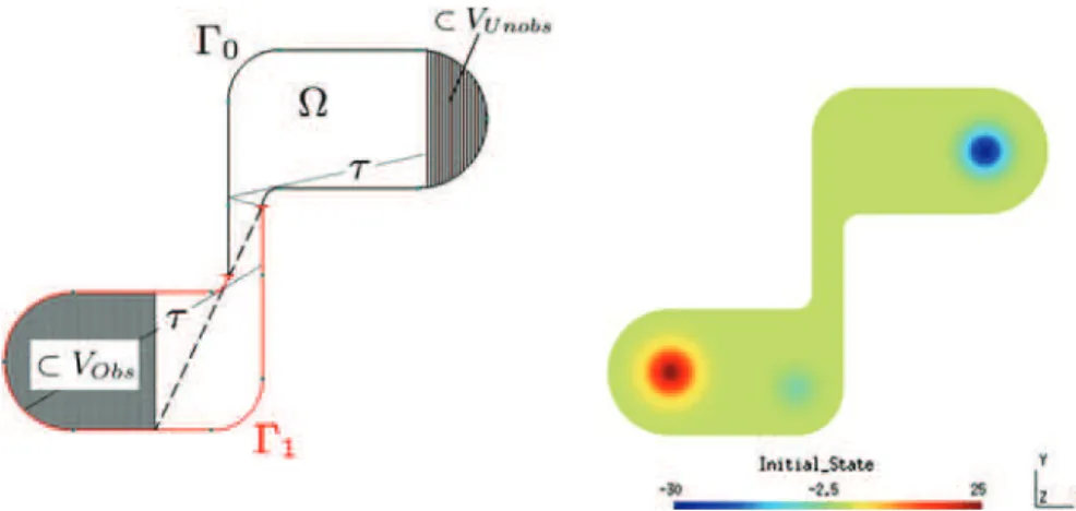
Fig. 1 An example of configuration in two dimensions and the initial state to reconstruct ¨ w+n(x, t ) − ∆wn+(x, t ) =0 ∀ x ∈ Ω, t ∈ (0, τ ), w+n(x, t ) =0 ∀ x ∈ Γ0, t ∈ (0, τ ), w+n(x, t ) = γ∂(−∆) −1w˙+ n(x, t ) ∂ν + γ y(x, t) + u(x, t) ∀ x ∈ Γ1, t ∈ (0, τ ), w+1(x,0) = 0 w˙1+(x,0) = 0 ∀ x ∈ Ω, w+n(x,0) = w−n−1(x,0), w˙n+(x,0) = ˙w−n−1(x,0) ∀ x ∈ Ω, n ≥ 2, and ¨ w−n(x, t ) − ∆wn−(x, t ) =0 ∀ x ∈ Ω, t ∈ (0, τ ), w−n(x, t ) =0 ∀ x ∈ Γ0, t ∈ (0, τ ), w−n(x, t ) = γ∂(−∆) −1w˙− n(x, t ) ∂ν − γ y(x, t) + u(x, t) ∀ x ∈ Γ1, t ∈ (0, τ ), w−n(x, τ ) = w+n(x, τ ), w˙n−(x, τ ) = ˙wn+(x, τ ) ∀ x ∈ Ω.
Denote Π the orthogonal projector from L2(Ω) ×H−1(Ω)onto VObs= Ran Φτd(we
do not show it explicitly). Then, from Corollary1.2, we have
' ' ' ' = wn−(x,0) ˙ wn−(x,0) > − Π = w0(x) w1(x) >''' ' L2(Ω)×H−1(Ω) −→ n→∞0.
Furthermore, the decay is exponential if and only ifRan Φτd is closed in L2(Ω) ×
H−1(Ω).
To illustrate Theorem4.1, consider the configuration on the left of Fig.1and let us try to reconstruct the initial state on the right of Fig.1, constituted of three bumps, with null initial velocity. For simplicity sake, we take u ≡ 0.
Then, we choose τ > 0 such that, using the geometric optic rays (see Bardos et al. [5]), we can reconstruct all initial data with support included in the left striped part,
and that no information can be obtained from the initial data with support included in the right striped part. In particular, we cannot expect to reconstruct the bump in the right top part of Ω.
Remark 4.2 It is well-known that uniform controllability/observability (with respect to the mesh size parameters) may fail after discretization (see for instance Zhang et al. [46]) due to high-frequency spurious modes. Using a numerical viscosity method, Ervedoza and Zuazua [14] proposed a time discretization preserving the uniform (in the time parameter) exponential stability of a damped wave equation.
More recently, García and Takahashi [17] used a finite-difference discretization in space for a one-dimensional wave equation. To avoid restrictions on the number of steps with respect to the mesh size, they add a vanishing viscosity in the numerical observers. They prove an estimate of the errors with respect to the mesh size and to the number of steps in the algorithm of [32].
In the case studied here, where we do not have exact observability, it is not clear if such a process can be used to tackle the spurious modes. Indeed, a further investigation of the discretization of VObsand its stability under the discretized algorithm should be done.
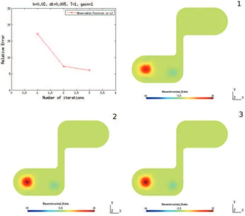
Fig. 2 Relative error of the “observable part of the position” in L2(Ω)and the reconstructions obtained after the first, second and third iterations
Remark 4.3 In presence of noisy measurement, we do not know if the stability of VObs under the discretized algorithm is preserved. It is more likely that this stability fails, leading to a deterioration of the reconstruction.
Using GMSH [20] and GetDP [13], we have implemented the algorithm with finite elements in space (parameter h = 0.02) and an unconditionally stable Newmark scheme in time (parameter 1t = 0.005), with γ = 1 and a time of observation τ = 1. We have obtained Fig. 2, where we can see the efficiency of the algorithm to reconstruct “the observable part” of the initial data (we take here the truncation on the bottom part of the figure). After only three iterations, we reach 6 % of relative error in L2(Ω).
References
1. Auroux D, Blum J (2005) Back and forth nudging algorithm for data assimilation problems. C R Math Acad Sci Paris 340(12):873–878
2. Auroux D, Blum J (2008) A nudging-based data assimilation method for oceanographic problems: the back and forth nudging (bfn) algorithm. Nonlinear Proc Geophys 15:305–319
3. Auroux D, Blum J, Nodet M (2011) Diffusive back and forth nudging algorithm for data assimilation. C R Math Acad Sci Paris 349(15–16):849–854
4. Baras JS, Bensoussan A (1987) On observer problems for systems governed by partial differential equations. No. SCR TR 86–47. Maryland University College Park, pp 1–26
5. Bardos C, Lebeau G, Rauch J (1992) Sharp sufficient conditions for the observation, control, and stabilization of waves from the boundary. SIAM J Control Optim 30(5):1024–1065
6. Bensoussan A (1993) Filtrage optimal des Systèmes Linéaires. Dunod
7. Blum J, Le Dimet F-X, Navon IM (2009) Data assimilation for geophysical fluids. In: Handbook of numerical analysis. Vol. XIV. Special volume: computational methods for the atmosphere and the Oceans, vol 14 of Handb. Numer. Anal. Elsevier, North-Holland, pp 385–441
8. Brezis H (2011) Functional analysis. Sobolev spaces and partial differential equations. Universitext. Springer, New York
9. Chapelle D, Cîndea N, De Buhan M, Moireau P (2012) Exponential convergence of an observer based on partial field measurements for the wave equation. Math Probl Eng. Art. ID 581053, 12
10. Couchouron J-F, Ligarius P (2003) Nonlinear observers in reflexive Banach spaces. ESAIM Control Optim Calc Var 9:67–104 (electronic)
11. Curtain RF, Weiss G (1989) Well, posedness of triples of operators (in the sense of linear systems theory). In: Control and estimation of distributed parameter systems (Vorau, (1988) volume 91 of Internat. Ser. Numer. Math. Birkhäuser, Basel, pp 41–59
12. Curtain RF, Weiss G (2006) Exponential stabilization of well-posed systems by colocated feedback. SIAM J Control Optim 45(1):273–297 (electronic)
13. Dular P, Geuzaine C GetDP reference manual: the documentation for GetDP, a general environment for the treatment of discrete problems.http://www.geuz.org/getdp/
14. Ervedoza S, Zuazua E (2009) Uniformly exponentially stable approximations for a class of damped systems. J Math Pures Appl (9) 91(1):20–48
15. Fink M (1992) Time reversal of ultrasonic fields-basic principles. IEEE Trans Ultrason Ferro Electric Freq Control 39:555–556
16. Fink M, Cassereau D, Derode A, Prada C, Roux O, Tanter M, Thomas J-L, Wu F (2000) Time-reversed acoustics. Rep Prog Phys 63(12):1933–1995
17. García GC, Takahashi T (2013) Numerical observers with vanishing viscosity for the 1d wave equation. Adv Comput Math 1–35
18. Gebauer B, Scherzer O (2008) Impedance-acoustic tomography. SIAM J Appl Math 69(2):565–576 19. Gejadze IY, Le Dimet F-X, Shutyaev V (2010) On optimal solution error covariances in variational
data assimilation problems. J Comput Phys 229(6):2159–2178
20. Geuzaine C, Remacle J-F (2009) Gmsh: a 3-D finite element mesh generator with built-in pre- and post-processing facilities. Int J Numer Methods Eng 79(11):1309–1331
21. Guo B-Z, Shao Z-C (2012) Well-posedness and regularity for non-uniform Schrödinger and Euler-Bernoulli equations with boundary control and observation. Quart Appl Math 70(1):111–132 22. Guo B-Z, Zhang X (2005) The regularity of the wave equation with partial Dirichlet control and
colocated observation. SIAM J Control Optim 44(5):1598–1613
23. Guo B-Z, Zhang Z-X (2007) On the well-posedness and regularity of the wave equation with variable coefficients. ESAIM Control Optim Calc Var 13(4):776–792
24. Ito K, Ramdani K, Tucsnak M (2011) A time reversal based algorithm for solving initial data inverse problems. Discret Contin Dyn Syst Ser S 4(3):641–652
25. Krstic M, Guo B-Z, Smyshlyaev A (2011) Boundary controllers and observers for the linearized Schrödinger equation. SIAM J Control Optim 49(4):1479–1497
26. Kuchment P, Kunyansky L (2008) Mathematics of thermoacoustic tomography. Eur J Appl Math 19(2):191–224
27. Le Dimet F-X, Shutyaev V, Gejadze IY (2006) On optimal solution error in variational data assimilation: theoretical aspects. Russ J Numer Anal Math Model 21(2):139–152
28. Liu K (1997) Locally distributed control and damping for the conservative systems. SIAM J Control Optim 35(5):1574–1590
29. Luenberger D (1964) Observing the state of a linear system. IEEE Trans Mil Electron 8:74–80 30. Moireau P, Chapelle D, Le Tallec P (2008) Joint state and parameter estimation for distributed
mechan-ical systems. Comput Methods Appl Mech Eng 197(6–8):659–677
31. Phung KD, Zhang X (2008) Time reversal focusing of the initial state for Kirchhoff plate. SIAM J Appl Math 68(6):1535–1556
32. Ramdani K, Tucsnak M, Weiss G (2010) Recovering the initial state of an infinite-dimensional system using observers. Automatica 46:1616–1625
33. Salamon D (1989) Realization theory in Hilbert space. Math Syst Theory 21:147–164
34. Shutyaev V-P, Gejadze IY (2011) Adjoint to the Hessian derivative and error covariances in variational data assimilation. Russ J Numer Anal Math Model 26(2):179–188
35. Smyshlyaev A, Krstic M (2005) Backstepping observers for a class of parabolic PDEs. Syst Control Lett. 54(7):613–625
36. Staffans O, Weiss G (2002) Transfer functions of regular linear systems. II. The system operator and the Lax-Phillips semigroup. Trans Am Math Soc 354(8):3229–3262
37. Staffans O, Weiss G (2004) Transfer functions of regular linear systems. III. Inversions and duality. Integral Equ Oper Theory 49(4):517–558
38. Teng JJ, Zhang G, Huang SX (2007) Some theoretical problems on variational data assimilation. Appl Math Mech 28(5):581–591
39. Tucsnak M, Weiss G (2009) Observation and control for operator semigroups. Birkhäuser Verlag, Basel 40. Weiss G (1989) The, representation of regular linear systems on Hilbert spaces. In: Control and estima-tion of distributed parameter systems (Vorau, (1988) vol 91 of Internat. Ser. Numer. Math. Birkhäuser, Basel, pp 401–416
41. Weiss G (1994) Regular linear systems with feedback. Math Control Signals Syst 7(1):23–57 42. Weiss G (1994) Transfer functions of regular linear systems. I. Characterizations of regularity. Trans
Am Math Soc 342(2):827–854
43. Weiss G, Curtain RF (2008) Exponential stabilization of a Rayleigh beam using collocated control. IEEE Trans Autom Control 53(3):643–654
44. Weiss G, Rebarber R (2000) Optimizability and estimatability for infinite-dimensional linear systems. SIAM J Control Optim. 39(4):1204–1232 (electronic)
45. Weiss G, Staffans OJ, Tucsnak M (2001) Well-posed linear systems–a survey with emphasis on con-servative systems. Int J Appl Math Comput Sci 11(1):7–33
46. Zhang X, Zheng C, Zuazua E (2009) Time discrete wave equations: boundary observability and control. Discret Contin Dyn Syst 23(1–2):571–604