Project no. 505428 (GOCE)
AquaTerra
Integrated Modelling of the river-sediment-soil-groundwater system; advanced tools for the management of catchment areas and river basins in the
context of global change Integrated Project
Thematic Priority: Sustainable development, global change and ecosystems
Deliverable No.: BASIN R3.26 (Meuse)
Title: Development of the Geer basin Hydrological model for climatic scenarios and first results about impacts evaluation
Due date of deliverable: May 2008 Actual submission date: May 2008
Start date of project: 01 June 2004 Duration: 60 months
Organisation name and contact of lead contractor and other contributing
partners for this deliverable:
P. Goderniaux1, S. Brouyère1,2, Ph. Orban1, A. Dassargues1 1
Group of Hydrogeology and Environmental Geology, 2Aquapôle ULg University of Liège, Building B52/3, 4000 Sart Tilman, Belgium Tel: +32.43.662377/ Fax: +32.43.669520, Serge.Brouyere@ulg.ac.be
Revision: H. Rijnaarts, J. Joziasse, J. Barth
Project co-funded by the European Commission within the Sixth Framework Programme (2002-2006)
Dissemination Level PU Public
PP Restricted to other programme participants (including the Commission Services) RE Restricted to a group specified by the consortium (including the Commission Services)
SUMMARY
MILESTONES REACHED (…….)
A surface – subsurface flow numerical model of the Geer basin (465 km²) has been implemented to assess the possible impacts of climate change on the groundwater resources. This model is physically-based, spatially-distributed and it integrates totally the groundwater and surface water. Simulations were performed using 6 climate change scenarios generated by the University of Newcastle-Upon-Tyne. These scenarios simulate changes in the amplitude, but also in the frequency and persistence of some meteorological events. First results show that, according the implemented flow model and the used climatic scenarios, significant decreases are expected in the groundwater levels (up to 12 meters) and in the surface water flow rates (reduction between 16% and 32%)
No milestones are associated to this deliverable
Using the meteorological data available for the Geer basin, HYDRO 1 has generated climate change scenarios which have been used as input to the hydrological model. This deliverable is of prime interest to the COMPUTE community as it presents one of the key case studies in AquaTerra.
Contents
1. Introduction with respect to objectives ________________________________________ 5 2. The Geer basin: general context _____________________________________________ 6 3. Modelling works __________________________________________________________ 8 3.1 Introduction __________________________________________________________ 8 3.2 Conceptual model _____________________________________________________ 8 3.3 Modelling tool ________________________________________________________ 9 3.4 Modelling setup ______________________________________________________ 10 3.4.1 Discretisation ________________________________________________________ 10 3.4.2 Parameterization ______________________________________________________ 12 3.4.3 Stresses _____________________________________________________________ 13 3.5 Calibration __________________________________________________________ 15 4. Simulation of climate change scenarios ______________________________________ 22
4.1 Climatic scenarios ____________________________________________________ 22 4.2 First results and conclusions ___________________________________________ 23 5. Conclusions and perspectives ______________________________________________ 24 6. References ______________________________________________________________ 27
Glossary
HydroGeoSphere Finite element calculation code for subsurface and surface flow and solute transport
Smectite clay Greenish marl constituting the basis of the Hesbaye chalk aquifer Multi (pluri) -annual variability Character of data time series in which cycles of periodicity superior
to one year can be observed.
FRAC3DVS Subsurface module of the code HydroGeoSphere. FRAC3DVS solves 3D, variably-saturated subsurface flow and solute transport equations in non-fractured or discretely fractured media (developed by the University of Waterloo and the University Laval, Canada) MODHMS simulator Calculation code for surface water – groundwater modeling
(HydroGeoLogic Inc.)
Van Genuchten functions Mathematical functions that describe relations between the water saturation, the pressure head and the relative permeability, in variably-saturated media
Leakance factor Parameter that regulates water flows between to domains.
Concerning surface – subsurface coupling in HydroGeoSphere, it is defined as the conductivity of the ground surface divided by the thickness of ground across which flow occurs.
Dirichlet condition Prescribed hydraulic head value (or pressure head). Neumann condition Prescribed water flux value.
Cauchy condition Linear relationship that specifies water fluxes according to pressure head variations. This condition is usually used to model interactions between river and aquifer
Zero-depth gradient condition Force the slope of the water level to equal the bed slope Critical depth condition Force the water depth at the boundary to be equal to the critical
depth
Transient calibration Model calibration performed through time with transient variables and stresses.
Field capacity Soil moisture remaining in the soil after natural drainage Wilting point Minimum soil moisture required for the plants not to wilt Thiessen polygons Polygons which boundaries are at equal distance between two
adjacent points. Thiessen polygons are drawn by joining the perpendicular bisector of each line joining two adjacent points Manning roughness
coefficients Empirical coefficients used to calculate surface flows
Control period Time period with climatic features corresponding to a ‘non climate change scenario’. The control period is used for comparison with ‘climate change scenario’ held on equivalent periods
1. Introduction with respect to objectives
In the framework of the AquaTerra project, the Geer basin (Belgium) has been chosen as a test site to study the impacts of climate change on groundwater resources. In order to make scientific assessments of these future impacts, the Hydrogeology Group of University of Liège (Belgium) is developing a spatially distributed, physically based, surface - subsurface hydrological model for this catchment.
Impacts of climate changes on water resources have been studied for several years in several scientific contexts. However, most of the studies are often restricted to surface water, oversimplifying of even neglecting the groundwater component. Furthermore, the scientific work performed on groundwater and climate change shows variable results. Though differences in the studied climate and aquifer types exert surely an influence, the way of considering climatic scenarios and representing the hydrogeology systems also surely contributes to results variability. Climate change impacts on groundwater reserves are linked to sensible processes and often too strong assumptions lead to high uncertainty. Chen et al. (2002) propose to estimate climate changes impacts on a Canadian aquifer thanks to an empirical model linking the piezometric variations and the water recharge represented as a linear function of precipitation and temperature. Likewise, most of the studies focussing on surface water (ex: Arnell, 2003) generally use simplistic transfer functions to represent exchanges between ground- and surface water. Such transfer functions are often oversimplified with regard to reality. They can possibly substitute more elaborated approaches if used in conditions defined and verified in the calibration step. They become more hazardous if stresses go beyond the calibration intervals, what surely happens for climate change issues. More elaborated models, based on physical principles, spatially distributed and taking into account the hydrogeologic processes allow more realistic calculation of groundwater fluxes. A reliable estimation of groundwater recharge is also crucial in the context of climate change impacts. It can be considered according to various degrees of complexity: from simple linear function of precipitation and temperature (Chen et al., 2002) to the application of "soil models" simulating groundwater flow and solute transport in the partially saturated zone (Allen et al. 2003, Brouyère et al. 2004). Finally, climate change scenarios used in the simulations are of high importance since they are the drivers of possible impacts on groundwater. In order to analyse climate variation effects on groundwater behaviour, Allen et al. (2003) performed a sensitivity analysis on temperature and precipitation. Other authors (Yussoff et al., 2002; Brouyère et al., 2004) use more sophisticated scenarios thanks to application, on historic data, of monthly scaling factors generated by recent results of the Intergovernmental Panel on Climate Change (IPCC) meteorological models
The ongoing work, consists in two main parts. First, a physically-based and spatially-distributed model is developed for Geer basin in the Walloon Region of Berlgium. This model is implemented at the catchment scale and it integrates totally surface flows with subsurface flows in the saturated and partially saturated zones, all these processes being solved simultaneously using the finite elements technique. This enables to better consider the interdependent aspects of the flow calculation in each domain and to obtain a more realistic representation of the whole system. Coupled approaches with separated or external calculation routines do not allow
such realism. Increasing and diversifying the number of observation data used for calibration (surface and subsurface data) enables to constrain more some terms of the water balance, like recharge or surface water – groundwater interactions, which are precisely crucial points in the context of climate change impacts assessment. In the integrated model developed for the Geer basin, water exchange terms between the surface and subsurface nodes are calculated internally at each time step. Similarly, the actual evapotranspiration is calculated internally as a function of the soil moisture at each node of the defined evaporative zone and at each time step.
Secondly, the estimation of direct climate change impacts on groundwater levels and river flow rates is examined by applying climate change scenarios on the developed Geer basin model. The climate scenarios have been generated by the University of Newcastle-Upon-Tyne and can take into account changes in the amplitude of precipitations and temperatures but also in the frequency and persistence of meteorological events.
2. The Geer basin: general context
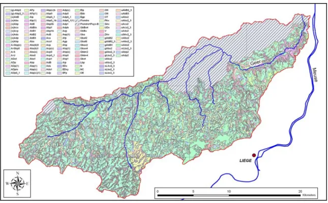
The Geer sub-catchment is located in eastern Belgium, North-West of the city of Liège, in the intensively cultivated 'Hesbaye' region. The hydrological basin extends over approximately 480 km², on the left bank of the Meuse River (Figure 1).
Figure 1 : Geer basin location and hydrographic limits
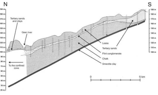
The geology of the Geer basin essentially consists in cretaceous chalky formations, dipping northward and limited at its base by impermeable smectite clay (Figure 2). Chalk layer thickness ranges from a few meters up to 70 m. It is divided in two parts by a thin layer of hardened chalk, called the 'Hardground'. A flint conglomerate, made of dissolved chalk residues, lies just over the chalk, with a
maximum thickness of 10 m. Tertiary sands are locally found above this conglomerate and a thick layer (up to 20 m) of quaternary loess is observed all over the catchment. North of the Geer River, tertiary sands and clays entirely cover chalks (Figure 2) (Orban et al. 2006a - R3.16).
Figure 2 : Geological cross-section in the Hesbaye aquifer (modified from Brouyère et al. 2004a). The vertical axis is exaggerated by a factor of 40
The chalk layers constitute the main aquifer formations in the catchment. The 'Hesbaye' aquifer is unconfined in most of the basin. In the northern part, near the Geer River, semi-confined conditions may prevail because of the loess quaternary deposits. North of the hydrologic Geer basin, the chalk aquifer is confined under tertiary clay and sands (Figure 2). Subsurface flow direction is from South to North and the aquifer is mainly drained by the Geer River flowing from West to East (Orban et al. 2006a - R3.16). The chalk formations are characterized by a dual porosity made of a porous matrix, which porosity can reach values up to 30 to 45 %, and fractures which generally represent less than 1% in volume. Fast preferential flows occur through the fractures while the porous matrix enables the storage of large volumes of water (Hallet, 1998; Brouyère, 2001). In the unsaturated zone, the thick loess layer controls the infiltration rate, resulting in smoothed recharge fluxes at the groundwater table and attenuation of seasonal fluctuations of hydraulic heads that are better characterized by multi-annual variations (Brouyère et al. 2004a). The Hesbaye aquifer is largely exploited for drinking water, mostly through more than 40 km lengths of pumping galleries located in the saturated chalk formation (Figure 1). The groundwater budget indicates groundwater losses, most probably through the northern catchment boundary, partly governed by groundwater pumping in the Flemish region of Belgium located North of the Geer basin. The Hesbaye aquifer suffers from severe nitrate contamination problems, essentially due to intense
agricultural activities. In the unconfined part of the aquifer, nitrate concentrations almost reach the drinking water limit of 50 mg/L (Batlle Aguilar et al. 2007).
3. Modelling works
3.1 Introduction
The Development and use of fully integrated surface – subsurface models is quite recent scientific work. Simulations usually need a lot of computer resources and most of the studies are limited to small catchments or short periods. Jones (2005) developed a model of a 75 km² catchment (Laurel Creek Watershed – Ontario, Canada) using more than 600 000 nodes. According to this work, transient simulations over a period of 1 month with daily time steps could take more than 4 days. Li et al. (2008) modelled a 286 km² catchment (Duffins Creek Watershed – Ontario, Canada) with more than 700 000 nodes and made transient simulations over 1 year periods with daily time steps. The integrated model of the Geer basin has to be developed for evaluating climate changes impacts. The catchment area is 465 km² and climate change scenarios are from 2010 to 2100. Using the same precision as for the model of Jones and Li is not possible because computing time would be too long. Nontheless, the objective of the model is not to simulate surface water at the river bed scale, but to have an accurate representation of the water balance terms at any time of the simulation. Using a model with fewer nodes may be sufficient to study climate change impacts and enables to limit computing times. The results presented in this report relate to one particular grid and further work will try to evaluate what could be the influence of different spatial and temporal discretisations.
3.2 Conceptual model
The Geer hydrographical catchment defines the limits of the modeled area. The smectite clay is considered as impervious and the contact between the clay and the chalk constitutes the basis of the model. Along the West, South and East boundaries, hydrogeological limits are considered to correspond to hydrographical limits. So, by definition, there are no water exchanges across these boundaries. On the contrary, groundwater fluxes through the north-western boundary must be taken into account. Along this border, hydrogeological limits differ from hydrographical ones, and water flows northwards in direction of the adjacent basin.
The Geer River, at its confluence with the Meuse River, is considered as the main outlet of the catchment. Elsewhere along the limits of the modeled area, no superficial water exchanges are observed, as these boundaries correspond to topographical limits.
Except near the Geer River and in the northern part of the catchment, where conditions become confined under tertiary and quaternary deposits, the saturated zone is exclusively located in the chalk formations. The vadose zone is then composed of unsaturated chalk, local sandy lenses and the thick loess layer. Hydraulic properties of the chalk formations vary vertically and laterally. Lower chalks (Campanian) are usually less permeable than upper chalks (Maastrichtian). According to Dassargues and Monjoie (1993), hydraulic conductivities vary from 10-5
higher hydraulic conductivity are observed and associated with 'dry valleys', oriented in the South – North direction. These zones, characterized by a higher degree of fracturation, are associated with slight drawdowns of hydraulic head. On the largest part of the Geer catchment, the tertiary deposits lying above the chalk represent unsaturated sand lenses of small extension. Their presence does probably not influence strongly the infiltration, more affected by the thick loess layer located above. On the contrary, at the North of the Geer River, tertiary deposits become thicker with some clearly clayey levels. These layers are responsible for the confined nature of the aquifer, in the northern part of the catchment, and must not be neglected. The thick loess layer, lying above the chalk and the tertiary deposits, is observed all over the catchment. Characterized by a low hydraulic conductivity (between 10-9 m.s-1 and 2×10⁻⁷ m.s-1 (Dassargues and Monjoie, 1993), it constitutes
an important part of the unsaturated zone and significantly slows down the water infiltration rate from the land surface to the chalky aquifer.
Stresses in the Geer catchment consist in precipitations, evapotranspiration and groundwater abstraction. Water collected through the 40 km of draining galleries represents the biggest part of groundwater abstraction in the Geer basin. Other pumping wells belonging to water supply companies or farmers are located all over the basin.
3.3 Modelling tool
The Geer basin hydrological model is under development using the finite elements code 'HydroGeoSphere' (Therrien et al. 2005), developed by the University of Laval and the University of Waterloo in Canada. This code allows making 3D spatially distributed simulations of variably saturated granular or fractured aquifers. It enables to fully integrate surface flow, subsurface flow and transport aspects, in a spatially distributed, physically-based manner. HydroGeoSphere is able to run with dynamic interactions between all sub-domains at each time step. It enables to partition rainfall into components such as evapotranspiration, run-off and infiltration. The code also allows calculating water infiltration or exfiltration between rivers and aquifers. All these interactions are particularly interesting in the context of climate change where the recharge processes are very sensible to climatic features and represent crucial elements for impacts estimation.
HydroGeoSphere is written in FORTRAN 95, using the control volume finite element approach. The module FRAC3DVS solves subsurface flow and transport equations. The surface module is based on the Surface Water Flow Packages of the MODHMS simulator. Richard's formulation is used to describe transient subsurface flow in variably saturated medium. A 2D depth-averaged approximation of the Saint Venant equations is used to describe and model surface water flows. In the subsurface domain, the hydraulic heads, the degrees of saturation, and the water fluxes are calculated at each node of the grid. In the surface domain, water thicknesses and flux values are calculated for each node of the 2D grid. The streams positions can be implicitly retrieved by considering the nodes where the water depth is not equal or very close to zero. Transport processes integrate advection, dispersion, retardation effects and decay. Newton Raphson iterations are used for resolving non linear equations.
3.4 Modelling setup
3.4.1 Discretisation
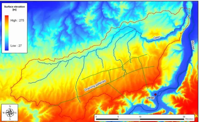
The hypotheses chosen in the conceptual model are used to build the three dimensional finite element mesh, made up of several layers of 6-nodes triangular prismatic elements. These elements have lateral dimensions of approximately 500 m. The top and bottom nodes layers represent the soil surface and the contact between smectite clay and chalk, respectively. Chalk formations are discretized using 3 layers of finite elements. Tertiary deposits and quaternary loess deposits are discretized using 3 layers of finite elements. The ground surface is discretized using 1 layer of 2D finite elements (Figure 3). The implemented model uses the ‘dual node approach’ to calculate water fluxes between the surface and subsurface nodes, as a function of the difference between surface and subsurface water heads and a leakance factor characterizing the properties of the soil. The elevation of the layers representing contacts between geologic formations (quaternary and tertiary deposits, chalk, smectite clay), is interpolated based on available information from existing boreholes. The elevations of the surface nodes are calculated using the Geer basin DTM (Digital Terrain Model) which pixels dimensions are 30 × 30 m (Figure 4). The total number of nodes is 6280.
Figure 4 : Digital terrain model of the Geer basin
Boundary conditions represent the strict application of the chosen hypothesizes in the conceptual model. Generally, three kinds of boundary conditions may be prescribed at subsurface nodes. They can be constant or vary according to time.
Dirichlet condition: prescribed hydraulic head values (or pressure head); exchanged fluxes between external and modeled domains are calculated according to these prescribed heads.
Neumann condition: prescribed water flux values; corresponding hydraulic heads are calculated during the simulation.
Cauchy condition: linear relationship between water fluxes and pressure head variations; this condition is usually used to model interactions between river and aquifer.
No-flow Neumann conditions are applied on subsurface nodes belonging to Western, Southern and Eastern boundaries. Cauchy conditions are applied on the subsurface nodes along the Northern boundary. This type of boundary condition enables to simulate groundwater losses in direction of the adjacent catchment located northward from the Geer basin.
For subsurface domains, HydroGeoSphere enables to prescribe several types of boundary conditions for surface water modeling.
Dirichlet condition: prescribed water depth values on nodes. Neumann condition: prescribed water flow rate values on nodes.
Zero-depth gradient condition: force the slope of the water level to equal the bed slope.
Critical depth condition: force the water depth at the boundary to be equal to the critical depth.
No-flow (Neumann) boundary conditions are prescribed along the hydrographical limits of the Geer basin. Critical-depth boundary conditions are prescribed at the nodes corresponding to the catchment outlet, at the confluence between the Geer and the Meuse Rivers.
3.4.2 Parameterization
The Geer basin model is parameterized for flow calculations. Further work will be devoted to update the model for transport purposes.
In the subsurface domain, used parameters are :
Full saturated hydraulic conductivity : K [L.T-1]
Total porosity : n [-]
Specific storage : Ss [L-1]
Van Genuchten parameters that define the partially saturated relations (pressure head vs saturation, relative hydraulic conductivity vs saturation) :
- Van Genuchten parameter α [-] - Van Genuchten parameter β [L-1] - Residual water saturation Swr [-]
In the surface domain, used parameters are :
Coupling length : Lc [L]
Manning roughness coefficients : nx, ny [L-1/3T]
The coupling length and the Manning coefficients respectively control infiltrations and runoff of surface water.
The model of Kristensen & Jensen (1975) is used by HydroGeoSphere to calculate the actual transpiration and evaporation, in function of the potential evapotranspiration and the soil moisture at each node of the evaporative zone. Parameters are :
Evaporation depth : Le [L]
Evaporation limiting saturations : θe1, θe2 [-]
Leaf area index : LAI [-]
Evaporation flow rates decrease within the evaporation depth, following a quadratic law. Full evaporation can occur if the water saturation is higher than θe1. No
evaporation occurs if water saturation is lower than θe2. Between these two limiting
saturations, evaporation decreases following a linear law. The LAI represent the cover of leaves over a unit area.
Root depth : Lr [L]
Transpiration fitting parameters : C1, C2, C3 [-]
Transpiration limiting saturations : Wilting point, Field capacity [-] Canopy storage parameter : cint [L]
Transpiration flow rates decrease within the root depth, following a quadratic law. Full transpiration can occur if the water saturation is higher than the Field capacity. No transpiration occurs if the water saturation is lower than the Wilting point. Between these two limiting saturations, transpiration decreases following a law governed by parameter C3. Cint accounts for the quantity of water that can be stored by the
canopy.
More details about the used parameters and subsequent relations can be found in Therrien et al. (2005).
3.4.3 Stresses
Stresses on the Geer catchment consist in precipitations, evapotranspiration and groundwater abstraction by the draining galleries and the pumping wells.
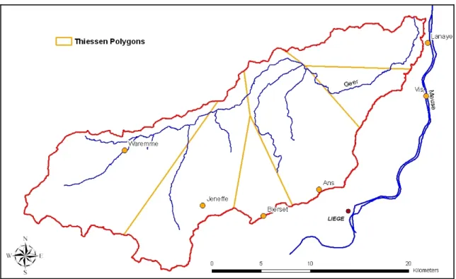
Historical climatic data are available for several stations located inside or in the vicinity of the Geer basin (Figure 5). Records begin from 1960, for the oldest stations, to 2005 (more details in Orban et al. 2006a). The following stations present complete 30 years time series, for precipitation (P). Temperature (T) and potential evapotranspiration (ETP) are available for Bierset and Maastricht stations.
Ans (P) (X = 232055 m, Y = 150597 m)1 Awirs (P) (X = 223700 m, Y = 144138 m) Bierset (T,P) (X = 226460 m, Y = 147928 m) Jeneffe (P) (X = 220260 m, Y = 149000 m) Maastricht (T, P) (X = 249561 m, Y = 179371 m) Visé (P) (X = 243005 m, Y = 160143 m) Waremme (P) (X = 212400 m, Y = 154500 m)
Except for the Maastricht station which is too far from the Geer basin, all data from these climatic stations are used as input of the model. The other stations present too short records periods or too important gaps of data. Precipitations are distributed on Geer basin using Thiessen polygons (Figure 6). Potential evapotranspiration data from the only Bierset station are used and extended to the whole catchment. Actual evapotranspirations are calculated by HydroGeoSphere using the model of Kristensen & Jensen (1975). Precipitations and potential evapotranspirations are applied on the surface node layer as transient specified fluxes.
1
Figure 5 : Location of available climatic data (from Orban et al. 2006a)
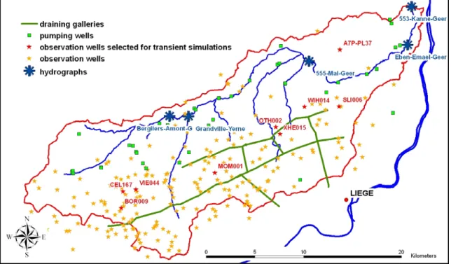
Extracted groundwater volumes, from the draining galleries and from the most important production wells (Figure 7), have been collected by the Walloon administration and are updated annually (for more details, see Orban et al., 2006a). According to Hallet (1998), extracted groundwater volumes represent between 6% and 11% of the annual precipitations. Transient volumetric flow rates are prescribed at each node of the 3D grid corresponding to the draining galleries or the pumping wells locations.
Figure 7 : pumping wells, draining galleries and observation points on the Geer basin
3.5 Calibration
The model calibration is performed using observed hydraulic heads and surface flow rates during the period 1967-2003. Hydraulic head data from more than 200 wells are available for the Geer basin (Figure 7). Although some of them present very few or irregular measurements, others have long and continuous data time series, sometimes for more than 30 years. River flow rates are available for five gauging stations (hydrographs) on the Geer and the Yerne rivers (Figure 7). Several laboratory tests and field tests (pumping tests, tracing experiments) were also carried out in the geologic formations of the Geer basin, and give some indicative values of hydraulic conductivities. Hallet (1998) , Brouyère (2001) and Brouyère et al. (2004a) also give orders of magnitude for some parameters of the Geer basin formations.
A preliminary calibration was first performed in steady state conditions, using two contrasted situations, corresponding to high and low groundwater levels (1967-1968 and 1991-1992). Results corresponding to the high groundwater levels configuration are then used as initial conditions for the transient simulations (‘year 1967’). The transient calibration between 1967 and 2003 is performed using the data from the 5 gauging stations and from 9 observation wells selected according to their
location and the length of their measured time series (Figure 7). In order to limit the computing times, monthly time steps are used.
In the subsurface domain, the parameters described in Chapter 3.4.2 are adjusted as follows. The results of the calibration are presented in Figure 8 and in Table 1.
Figure 8 : Zones of hydraulic conductivity for the 3 chalk layers (results of calibration)
Van Genuchten parameters are defined according to values given by Brouyère (2001) and Brouyère et al. (2004a). Table 2 summarizes the values used for the chalk and loam formations.
In the surface domain, the parameters defined in Chapter 3.4.2 are adjusted according to the information given by the soil and land use maps (Figure 9 and Figure 10). The Manning roughness coefficients are defined for 3 categories of land use, namely rural, urban and forested. Values can be found in Jones (2005), Li et al. (2008), Hornberger et al. (1998). Predefined values are shown in Table 3. However, with these range of values, it turned out impossible to obtain a good calibration of the simulated surface flow rates. More satisfying results were obtained using roughness coefficients values of one order of magnitude higher. The abnormal values of these empirical coefficients could be due to the coarser spatial and temporal discretisation than in usual hydrological models. Further more detailed simulations will be held to investigate the effects of the cell size and time steps. The coupling length should be
adjusted according to soil type and thickness (Figure 10). However, the cell size is globally much bigger than the soil type polygons in Figure 10) which implies some difficulties in defining and differentiating cell properties. Moreover, during the calibration step, the coupling length appeared to be quite insensible. Therefore, given these observations, the coupling has been uniformly set to 0.01 m for the whole surface domain.
Zone
number name Saturated hydraulic conductivity [m s-1]
2 loess 1×10⁻⁸ ch alk inf. 3 north-east inf. 2×10⁻⁵ 4 south-east inf. 2×10⁻⁶ 5 chalk inf. 4×10⁻⁵ 6 south inf. 2.75×10⁻⁵
7 dry valley inf. 2×10⁻⁴
8 gallery inf 1×10⁻³ cha lk i nt. 9 chalk int. 1×10⁻⁴ 10 north-east int. 1×10⁻⁶ 11 south-east int. 5×10⁻⁸ 12 south int. 1×10⁻⁵
13 dry valley int. 2×10⁻⁴
14 gallery int. 1×10⁻³
chalk su
p. 15 chalk sup. 1×10⁻⁴
16 north east sup. 1×10⁻⁴
17 south sup. 1×10⁻⁴
18 dry valley sup. 2×10⁻⁴
Table 1 : Hydraulic conductivities values of the calibrated zones (results of calibration)
α [-] β [l-1] S
wr [-] n [-] Ss [L-1]
Chalk formations 0.099 1.10 0.023 0.44 1×10⁻⁴
Loam formations 0.076 1.16 0.024 0.41 1×10⁻⁴
Table 2 : Van Genuchten parameters, total porosity and specific storage
X friction [L-1/3T] Y friction [L-1/3T]
Rural 0.3 0.3
Urban 0.03 0.03
Forested 0.6 0.6
Figure 9 : Land use map of the Geer basin
Figure 10 : Soil map of the Geer basin2
(Data available only for the Walloon part of the Geer basin, not available for shaded areas)
2 © Direction Générale de l’Agriculture (Ministère de la Région Wallonne). Projet de Cartographie Numérique des sols de Wallonie (PCNSW). Projet du Gouvernement Wallon (GW VIII/2007/Doc.58.12/12.07/B.L & GW VII/2000/Doc.1331/07.12/JH.)
The parameters used to calculate the actual evapotranspiration (Kristensen & Jensen, 1975; see Chapter 3.4.2) are defined using values found in the literature. The limiting saturations corresponding to the wilting point and field capacity are specified as the saturations corresponding to pF values3 equal to 4.2 and 2.5, as found in Brouyère (2001). Root depths are evaluated using values given by Canadell et al. (1996). Evaporation depth is specified as 2 m uniformly over the whole catchment (Table 4). Values for the Leaf Area Index (LAI) are given by Scurlock et al. (2001), Asner et al. (2003), Vasquez and Feyen (2003), Li et al. (2008). Breuer et al. give maximum and minimum values of the LAI throughout the year. LAI values specified in the Geer basin model are shown in Table 4.
Root depth Lr [L] Evaporation depth Le [L] LAI [-]
Rural crop (temperate) 2.1 2 4.22
Rural grassland (temperate) 2.6 2 2.50
Rural broadleaf deciduous
forested (temperate) 5.2 2 2.64
Urban 0 2 0.40
Table 4 : Maximum root depths, evaporation depths and Leaf Area Index
Few references exist concerning the C1, C2 and C3 empirical transpiration fitting parameters of the model of Kristensen and Jensen (1975). Li et al. (2008) made a state-of-the-art of used values. For the Geer basin model, specified values of C1, C2 and C3 as well as the coefficient of canopy storage interception Cint, are shown in
Table 5.
C1 [-] C2 [-] C3 [-] Cint [L]
0.3 0.2 10 1×10⁻⁵
Table 5 : transpiration fitting parameters and canopy storage interception
Results of the steady state and transient simulations, using the calibrated parameters, are shown in Figure 11 to Figure 14. Figure 11 presents the computed hydraulic saturations in the subsurface domain for the steady state simulation corresponding to the high groundwater levels configuration. Similarly, Figure 12 shows the computed water thicknesses at each node of the surface domain. The Yerne and the Geer rivers can be easily identified, as corresponding to the highest water thicknesses. Results presented in Figure 11 and Figure 12 are used as initial conditions for the transient simulations from 1967 to 2003. Figure 13 presents the computed and observed transient hydraulic heads for the 9 selected observation
3
wells. Figure 14 presents the computed and observed transient flow rates for the ‘Kanne’ gauging station located at the outlet of the aquifer. The results corresponding to the 4 other gauging stations are not shown in this deliverable since they are quite similar to the results at ‘Kanne’ gauging station. The computed flow rates are of the same order of magnitude as the observed flow rates. Computed values match particularly well observed values during summers (low flow rates, recession periods). Imperfections remains for the winter periods for which computed flow rates are too high in comparison with observed flow rates. However, globally speaking, computed and observed hydraulic heads match quite well. Computed hydraulic heads reproduce satisfactorily multi-annual variations in groundwater levels, even though some observation wells (e.g. MOM001 and A7-PL37) still present important gaps between observed and computed piezometric heads. Seasonal variations, as calculated by the model, are slightly too high at some observation wells, especially for ‘VIE044’, which groundwater level is close to the ground surface, and ‘A7-PL7’, which presents unexpected abrupt seasonal variations. Globally, the quality of the calibration can be considered as better in the upstream part of the Geer basin. Table 6 presents the mean water balance terms for the simulation performed between 1967 and 2003. Further work will be dedicated to improve the calibration.
Figure 11 : hydraulic saturation calculated for the subsurface domain (results for the steady state simulation). The red colour relates to the saturated zone.
Figure 13 : transient calibration for the surface flow rates of Kanne gauging station (outlet)
Rain evapotransp. Actual North boundary Outlet (‘Kanne’) abstraction Water Water balance error
mm/year 798.6 -538.3 -37.5 -202.5 -24.1 3.8
% 100 -67.4 -4.7 -25.4 -3.0 0.5
Table 6 : mean water balance terms for the period 1967-2003
4. Simulation of climate change scenarios
As already mentioned, the integrated Geer basin model has been specially developed to assess the possible impacts of climate changes on groundwater resources. Simultaneous modelling of surface and subsurface flow enables to devote special care to recharge processes, which are crucial points in the context of climate changes.
4.1 Climatic scenarios
In order to evaluate the direct impacts of climate changes on water resources, the University of Newcastle upon Tyne has generated 6 climate change scenarios for precipitations and temperatures. These climate change scenarios simulate changes in the amplitude of precipitations and temperatures but also in the frequency and persistence of some meteorological events like drought or flood periods. The 6 scenarios have been generated for 3 different periods (2010-2040, 2040-2070, 2070-2100) using daily time steps, with a simple bias-correction method (Wood et al., 2004; Blenkinsop et al., 2008) of Regional Climate Models data (RMC) from the FP5 PRUDENCE project (Prediction of Regional scenarios and Uncertainties for Defining European Climate change risk and Effects, http://www.prudence.dmi.dk). The scenarios represent a stationary climate over each 30-year period. Table 7 summarizes the names and associated Regional Climate Model (RCM) and Global Climate Models (GCM) for the 6 used scenarios. Precipitations and temperatures have been generated for the available climatic stations shown in Figure 5, using observed data from 1961 to 1990 as a baseline for calculation. As explained in Chapter 3.4.3, only stations presenting reasonable and complete records time series have been used as input of the model (6 stations for precipitations, 1 station for temperatures and potential evapotranspiration). Generally, climate change scenarios show an increase in temperature all over the year, an increase in precipitations during winters and a decrease in precipitations during summers. Statistics for ‘Waremme’ (precipitations) and ‘Bierset’ (temperatures) climatic stations, for the 2070-2100 time period are presented at Figure 15 and Figure 16. Statistics for the 2010-2040 and 2040-2070 time periods present intermediate values and follow similar seasonal trends. First results include simulations for the 5 climate change scenarios HS1, ecscA2, adhfa, HCA2 and MPIA2. The scenario DE6 uses a slightly different calendar and the corresponding simulation has not been performed yet.
INST RCM GCM A2 SCENARIO PRUDENCE ACRONYM AQUATERRA ACRONYM
DMI HIRHAM HadAM3H A2 HS1 HIRHAM_H_A2
DMI HIRHAM ECHAM4/OPYCA2 ecscA2 HIRHAM_E_A2
HC HadRM3P HadAM3P adhfa HAD_H_A2
SMHI RCAO HadAM3H A2 HCA2 RCAO_H_A2
SMHI RCAO ECHAM4/OPYCA2 MPIA2 RCAO_E_A2
Météo-France Arpège Observed SST DE6 ARPEGE_H_A2
Figure 15 : monthly precipitation variations (mm) for each climate change scenario (period 2070-2100)
Figure 16 : monthly temperature variations (°C) for each climate change scenario (period 2070-2100)
4.2 First results and conclusions
Using the calibrated model and the generated climatic scenarios, simulations were run to evaluate direct climate change impacts for the 3 periods 2010-2040, 2040-2070 and 2070-2100. This chapter presents first results and will be updated in the last deliverable. First results and conclusions show a significant decrease in groundwater levels, compared to the groundwater levels computed for the control period, without climate change. Variations are visible at a multi-annual scale. Amplitudes of these variations depend on the location in the Geer basin, on the used climate change scenario and on the considered time intervals. Figure 17 presents the computed hydraulic head evolution in the observation well ‘OTH002’ for the control
period and for each climate change scenario. Concerning the surface water discharges, simulations with climate changes show little amplitude variations for the high water discharge peaks. On the other hand, surface water time series would be characterized by stronger and longer periods of low water discharge. Figure 18 presents the computed river flow rates at the outlet of the Geer basin (‘Kanne’ gauging station) for the control period and for the climate change scenario ‘ecscA2’. Results for the other gauging stations and for the other climate change scenarios present similar patterns. Table 8 presents the amplitude and variations of water balance terms for each climate change scenario during each considered time period. The examination of these values clearly shows that, according to this flow model and the used climate change scenarios, the evapotranspiration term is expected to take more and more importance. Similarly, water flow rates at the outlet of the basin (‘Kanne’ gauging station) are expected to decrease between 16% and 38% for the period 2070-2100. For the same volumes of collected water (for the city of Liège located out of the Geer basin) the water abstraction term takes more importance in the water balance as annual rainfalls are expected to decrease in the next decades. Differences appear between the control period terms and the values presented in Table 6. This is explained by the way the potential evapotranspiration is calculated. For the calibration step, ETP used as input to the model were obtained from the Royal Meteorological Institute of Belgium, based on a relatively sophisticated calculation algorithm. For the climate change simulations, ETP have been calculated with the Thornthwaite equation, since temperatures only are provided by the climate change scenarios. Differences are observed between these two evapotranspiration series, especially during summers. To make the analysis more consistent, further work will be devoted to standardize the way of calculating the ETP. New climate change scenarios with ETP time series could possibly be generated.
5. Conclusions and perspectives
A surface – subsurface water flow model of the Geer basin has been developed to assess the possible impacts of climate change on the groundwater resources. This model is physically-based, spatially-distributed and it integrates totally the groundwater and surface water components, incorporating some properties of the land use and soil types. This way of modelling enables to represent more realistically the hydrologic system. More specifically, special care is devoted to groundwater – surface water interactions and recharge processes, which are particularly important in the context of climate changes. The model has been calibrated using observations of hydraulic heads and surface water flow rates for the period 1967-2003. Simulations were performed using 6 climate change scenarios generated by the University of Newcastle-Upon-Tyne. These scenarios simulate changes in the amplitude, but also in the frequency and persistence of meteorological events. First results show that, according the implemented flow model and the used climatic scenarios (toward dryer summers), significant decreases are expected in the groundwater levels and in the surface water flow rates.
The results and tools presented above are highly important for river basin management as groundwater storage will be one of the key measures to mitigate decrease of water availability due to climate change. With our work we have provided an essential tool to predict and plan groundwater abstraction in the future. Improvements of the model could include higher resolution of input data especially
more detailed information on demographic, agricultural and industrial development, while more empirical details for the role of plants in water balances is needed.
Further work will be devoted to improve some aspects of the model and to perform more advanced analysis. The main aspects are listed below :
- Improvement of the calibration, especially at the level of the surface domain and the first meters of the subsurface domain.
- Evaluation of the influence of the temporal and spatial discretisations on the model performances.
- Implementation of a transport model.
Rain evapotransp. Actual Flux out of North boundary Flux out of main outlet (‘Kanne’) Water abstraction
Control period mm/year 801.1 -463.0 -40.9 -273.2 -24.0
% 100 -57.8 -5.1 -34.1 -3.0 2010-2040 HS1 mm/year 773.1 -460.8 -39.4 -248.2 -24.0 % 100 -59.6 -5.1 -32.1 -3.1 ecscA2 mm/year 777.4 -468.8 -38.9 -241.8 -24.1 % 100 -60.3 -5.0 -31.1 -3.1 adhfa mm/year 768.1 -449.3 -39.2 -254.2 -23.8 % 100 -58.5 -5.1 -33.1 -3.1 HCA2 mm/year 785.3 -460.2 -39.3 -259.9 -24.3 % 100 -58.6 -5.0 -33.1 -3.1 MPIA2 mm/year 785.3 -463.3 -39.3 -258.4 -24.3 % 100 -59.0 -5.0 -32.9 -3.1 2040-2070 HS1 mm/year 743.0 -462.1 -38.6 -220.7 -23.8 % 100 -62.2 -5.2 -29.7 -3.2 ecscA2 mm/year 755.9 -473.2 -37.8 -222.2 -24.2 % 100 -62.6 -5.0 -29.4 -3.2 adhfa mm/year 733.0 -455.9 -38.1 -217.7 -24.2 % 100 -62.2 -5.2 -29.7 -3.3 HCA2 mm/year 767.41 -468.1 -38.4 -238.7 -23.8 % 100 -61.0 -5.0 -31.1 -3.1 MPIA2 mm/year 772.4 -471.2 -38.6 -240.2 -23.9 % 100 -61.0 -5.0 -31.1 -3.1 2070-2100 HS1 mm/year % ecscA2 mm/year 720.1 -462.3 -36.7 -197.3 -24.5 % 100 -64.2 -5.1 -27.4 -3.4 adhfa mm/year 681.6 -453.9 -36.8 -169.7 -23.9 % 100 -66.6 -5.4 -24.9 -3.5 HCA2 mm/year 741.6 -465.0 -37.1 -215.8 -24.5 % 100 -62.7 -5.0 -29.1 -3.3 MPIA2 mm/year 750.2 -459.9 -37.5 -228.1 -24.0 % 100 -61.3 -5.0 -30.4 -3.2
Figure 18 : flow rates evolution at gauging station 'Kanne' for climate change scenario 'ecscA2'
6. References
Batlle Aguilar J., Orban Ph., Dassargues A., Brouyère S., 2007. Identification of groundwater quality trends in a chalky aquifer threatened by intensive agriculture. Hydrogeology Journal Vol. 15-8, pp. 1615-1627
Blenkinsop S., Burton A., Fowler H., Kilsby C., Van Vliet M., 2008. Production of probabilistic climate scenarios for AquaTerra case study catchments. Deliverable H1.11. AquaTerra (Integrated Project FP6 no 505428), pp. 54.
Broers H.P., Visser A., Pinault J.-L., Guyonnet D., Dubus I.G., Baran N., Gutierrez A., Mouvet C., Batlle Aguilar J., Orban Ph, Brouyère S., 2004. Report on extrapolated time trends at test sites. Deliverable T2.4. AquaTerra (Integrated Project FP6 no 505428), pp. 78.
Brouyère S., 2001. Etude et modélisation du transport et du piégeage des solutés en milieu souterrain variablement saturé (study and modelling of transport and retardation of solutes in variably saturated media) (In French). PhD thesis. Faculté des Sciences Appliquées. Laboratoire de géologie de l'ingénieur, d'Hydrogéologie et de Prospection géophysique. Université de Liège. Liège (Belgium). pp. 640. Brouyère S., 2006. Modelling the migration of contaminants through variably
saturated dual-porosity, dual-permeability chalk. Journal of Contaminant Hydrology, 82, pp. 195-219.
Brouyère S., Dassargues A., Hallet V., 2004a. Migration of contaminants through the unsaturated zone overlying the Hesbaye chalky aquifer in Belgium: a field investigation. Journal of Contaminant Hydrology, 72, pp. 135-164.
Brouyère S., Carabin G., Dassargues A., 2004b. Climate change impacts on groundwater resources: modelled deficits in a chalky aquifer, Geerbasin, Belgium. Hydrogeology Journal, 12, pp. 123-134.
Canadell J., Jackson R.B., Ehrlinger J.R., Mooney H.A., Sala O.E., Schulze E.D.,1996. Maximum rooting depth of vegetation types at the global scale, Oecologia, Vol. 108. pp. 583-595
Dassargues A., Monjoie A., 1993. The chalk in Belgium. In: Downing RA, Price M., Jones G.P. (eds). The hydrogeology of the chalk of north-west Europe. Clarendon Press, Oxford, UK, pp. 153-269.
De Wit M.J.M., Warmerdam P.M.M., Torfs P.J.J.F., Uijlenhoet R., Roulin E., Cheymol A., Van Deursen W.P.A., Van Walsum P.E.V., Ververs M., Kwadijck J.C.J., Buiteveld H., 2001. Effect of climate change on the hydrology of the river Meuse. Waveningen University. Environmental Sciences. Water Resources Rep., 108, pp. 134.
Eheart J.W., Tornil D.W., 1999. Low-flow frequency exacerbation by irrigation withdrawal in the agricultural Midwest under various climate change scenarios. Water Resources Research, 35(7), pp. 2237-2246.
Fowler H. J., Kilsby C. G., O'Connel P. E., 2003. Modelling the impacts of climatic change and variability on the reliability, resilience, and vulnerability of a water resource system. Water Resources Research, Vol. 39 – 8.
Hallet V., 1998. Etude de la contamination de la nappe aquifère de Hesbaye par les nitrates: hydrogeologie, hydrochimie et modélisation mathématique des écoulements et du transport en milieu saturé (Contamination of the Hesbaye aquifer by nitrates: hydrogeology, hydrochemistry and mathematical modelling) (in French). PhD thesis. Faculté des Sciences. Université de Liège. Liège (Belgium), pp. 361.
Hornberger M.G., Raffensperger J.P., Wiberg P.L., Eshleman K.L., 1998. Elements of Physical Hydrology. JHU Press. pp. 312.
Jones J-P., 2005. Simulating Hydrologic Systems Using a Physically-based Surface-Subsurface Model: Issues Concerning Flow, Transport and Parameterization. PhD Thesis. University of Waterloo (Canada). pp. 145.
Kristensen K.J., Jensen S.E., 1975. A Model For Estimating Actual Evapotranspiration From Potential Evapotranspiration. Nordic hydrology, Vol. 6. pp. 170-188.
Li Q., Unger A.J.A., Sudicky E.A., Kassenaar D., Wexler E.J., Shikaze S., 2008. Predicting the multi seasonal Response of a Large-Scale Watershed with 3D Physically-based Hydrologic Model. Journal of Hydrology. (Accepted manuscript) Orban Ph., Batlle Aguilar J., Goderniaux P., Dassargues A., Brouyère S., 2006a.
Description of hydrogeological conditions in the Geer sub-catchment and synthesis of available data for groundwater modelling. Deliverable R3.16. AquaTerra (Integrated Project FP6 no 505428), pp. 22.
Orban Ph., Brouyère S., 2006b. Groundwater flow and transport delivered for groundwater quality trend forecasting by TREND T2. Deliverable R3.18. AquaTerra (Integrated Project FP6 no 505428), pp. 20.
Therrien R., McLaren R.G., Sudicky E.A., Panday S.M., 2005. HydroGeoSphere. A three-dimensional numerical model describing fully-integrated subsurface and surface flow and solute transport.
Wood A.W., Leung L.R., Sridhar V., Lettenmaier, D.P., 2004. Hydrologic implications of dynamical and statistical approaches to downscaling climatemodel outputs. Climatic Change, Vol. 62, pp. 189-216.
Yussof I., Hiscock K. M., Conway D., 2002. Simulation of the impacts of climate change on groundwater resources in eastern England. Sustainable Groundwater Development. Geological Society, London Special Publications, Vol. 193, pp. 325-344.