Draft overview paper on trend analysis in groundwater summarizing the main results of TREND2 in relation to the new Groundwater Directive

Texte intégral

(1)Project no. 505428 (GOCE). AquaTerra Integrated Modelling of the river-sediment-soil-groundwater system; advanced tools for the management of catchment areas and river basins in the context of global change Integrated Project Thematic Priority: Sustainable development, global change and ecosystems. Deliverable No.: TREND2.12. Title: Draft overview paper on trend analysis in groundwater summarizing the main results of TREND2 in relation to the new Groundwater Directive Due date of deliverable: 15 September 2007 Actual submission date: 15 September 2008. Start date of project: 01 June 2004. Duration: 60 months. Organisation name and contact of lead contractor and other contributing partners for this deliverable. Broers H.P1, Visser A.2,(eds.), Bierkens M.F.P.2, Dubus I.G3, Pinault J.L.3, Surdyk N. 3, Guyonnet D. 3 Batlle Aguilar J.4, Brouyere S.4, Goderniaux P.4, Ph. Orban4, Korcz M6, Bronder J.6, Dlugosz J.6, Odrzywolek M.6 1 Netherlands Organisation for Applied Scientific Research TNO, Division Groundwater and Soil, Princetonlaan 6, P.O. Box 80015, 3508 TA Utrecht, The Netherlands. E-mail: h.broers@tno.nl (lead partner) 2 Universiteit Utrecht, Faculty of Geographical Sciences, Budapestlaan 4, 3584 CD Utrecht, The Netherlands. 3 BRGM, Water Division, BP 6009, 45060 Orléans Cedex 2, France. 4 HG-ULg, University of Liege, Building B52/3, 4000 Sart Tilman, Belgium. 6 Institute for Ecology of Industrial Areas, ul. Kossutha 6, 40-844 Katowice, Poland. Revision: M.H. Gerzabek / J. Barth Project co-funded by the European Commission within the Sixth Framework Programme (2002-2006) Dissemination Level Public PU X Restricted to other programme participants (including the Commission Services) PP Restricted to a group specified by the consortium (including the Commission Services) RE Confidential, only for members of the consortium (including the Commission Services) CO.

(2) SUMMARY The current document provides a draft manuscript of a scientific paper to be submitted to an international peer reviewed journal. The paper provides an overview on trend analysis in groundwater summarizing the main results of TREND2 in relation to the new Groundwater Directive.. MILESTONES REACHED T2.12: Draft overview paper on trend analysis in groundwater summarizing the main results of TREND2 in relation to the new Groundwater Directive.. 2.

(3) 1. Comparison of methods for the detection and extrapolation. 2. of trends in groundwater quality. 3 4. Abstract. 5. Land use changes and the intensification of agriculture since 1950 have resulted in a. 6. deterioration of groundwater quality in most EU countries. For the protection of. 7. groundwater quality it is necessary to (1) assess the current groundwater quality. 8. status, (2) detect changes or trends in groundwater quality, (3) assess the threat of. 9. deteriorating groundwater quality and (4) predict future changes in groundwater. 10. quality. A variety of tool can be used to detect and extrapolate trends in groundwater. 11. quality, ranging from simple linear statistics to distributed 3D groundwater. 12. contaminant transport models. For this paper we compared four methods for the. 13. detection and extrapolation of trends in groundwater quality: (1) statistical methods,. 14. (2) groundwater dating, (3) transfer functions, and (4) deterministic models. The choice of the method for trend detection and extrapolation should firstly. 15 16. be made on the basis of the system under study, and secondly on the available. 17. resources and goals. For trend detection in groundwater quality, the most important. 18. difference between groundwater bodies is whether the character of the subsurface or. 19. the monitoring system causes mixing of groundwater with different travel times. We. 20. conclude that there is no single optimal method to detect trends in groundwater. 21. quality across widely differing catchments.. 22 23. 1.. Introduction. 24. Land use changes and the intensification of agriculture since 1950 have resulted in. 25. increased pressures on natural systems. For example, the diffuse pollution of 3.

(4) 26. groundwater with agricultural contaminants like nitrate and pesticides has resulted in. 27. a deterioration of groundwater quality. In general, the pressure of agricultural. 28. contaminants on the groundwater has increased since 1950, resulting in an increasing. 29. surplus of N applied to agricultural land. Following national legislation, the pressure. 30. decreased since the mid-1980s in most EU countries, resulting in a very similar. 31. evolution of the contamination history for diffuse pollution by agriculture in European. 32. countries and the US (Broers et al., 2004a). The transfer of these contaminants to. 33. deeper groundwater and surface water represents a major threat to the long-term. 34. sustainability of water resources across the EU and elsewhere.. 35 36. [Figure 1]. 37 38. For the protection of groundwater quality, legislators will ask the scientific. 39. community to (1) assess the current groundwater quality status, (2) detect changes or. 40. trends in groundwater quality, (3) assess the threat of deteriorating groundwater. 41. quality by relating them to historical changes in land use, (4) predict future changes in. 42. groundwater quality, by extrapolating present day trends and possibly predict trend. 43. reversal in response to legislation aimed at protecting groundwater quality.. 44. So far, the awareness of the threat to groundwater quality has led to the. 45. installation of groundwater quality monitoring networks (Almasri and Ghabayen,. 46. 2008; Almasri and Kaluarachchi, 2004; Broers, 2002; Daughney and Reeves, 2005;. 47. Hudak, 2000; Lee et al., 2007; Van Maanen et al., 2001) providing time series of. 48. groundwater quality. These time series have been used to detect changes in. 49. groundwater quality (Batlle-Aguilar et al., 2007; Broers et al., 2005; Broers and van. 4.

(5) 50. der Grift, 2004; Burow et al., 2007; Daughney and Reeves, 2006; Reynolds-Vargas et. 51. al., 2006; Stuart et al., 2007; Xu et al., 2007).. 52. In practice it is difficult to detect trends in groundwater quality for a number. 53. of reasons. Most often the period of interest is longer than the period of record (Loftis,. 54. 1996) and available time series are rather short and sparse because of the high cost of. 55. sampling and analysis. This limits the available statistical methods to simple linear. 56. statistics, rather than more complex time series analysis tools. Other factors. 57. complicating trend detection are:. 58. . contaminants towards monitoring location by groundwater flow. 59 60. . variations in application of contaminants at the ground surface, in space and time. 61 62. variations in the duration and pathways of the transport of. . (partial) degradation of contaminants in the subsurface. 63. The long travel times of contaminants through the groundwater system. 64. towards the monitoring location further complicates the detection of trends. The travel. 65. time of sampled groundwater may be uncertain, in particular because the groundwater. 66. sample may represent a range of groundwater travel times. Decreasing the uncertainty. 67. of the travel time by relating measured concentrations to the time of recharge often. 68. reveals clearer trends (Bohlke et al., 2002; Laier, 2004; MacDonald et al., 2003;. 69. Tesoriero et al., 2005; Wassenaar et al., 2006).. 70. To assess whether an upward trend in the concentration of a contaminant will. 71. continue to threaten groundwater quality, trends in groundwater quality can be related. 72. to changing land use pattern (Gardner and Vogel, 2005; Jiang et al., 2006; Lapworth. 73. et al., 2006; Ritter et al., 2007), and future trends can be predicted based on land use. 74. scenarios (Almasri and Kaluarachchi, 2005; Di et al., 2005). Eventually, trends in. 5.

(6) 75. groundwater quality may be predicted using a distributed 3D groundwater. 76. contaminant transport models (Almasri and Kaluarachchi, 2007; Refsgaard et al.,. 77. 1999; Van der Grift and Griffioen, 2008).. 78. This shows that a variety of tool can be used to detect and extrapolate trends in. 79. groundwater quality, ranging from simple linear statistics to distributed 3D. 80. groundwater contaminant transport models. The efficiency of these tools depends on. 81. several factors like the availability of groundwater quality data, the character of the. 82. groundwater flow system, and the available resources for trend assessment. One. 83. important factor for the success of trend detection in groundwater quality is whether. 84. the character of the groundwater flow system causes mixing of groundwater, for. 85. example in dual porosity systems, and whether the groundwater sample contains a. 86. mixture of groundwater, for example from springs or production wells.. 87. The aim of this comparison study was to assess the capabilities and efficiency. 88. of various tools to detect and extrapolate of trends in groundwater quality in a variety. 89. of different groundwater systems, ranging from unconsolidated unconfined aquifers to. 90. fissured dual porosity systems. For this paper we compared four sorts of methods for. 91. the detection and extrapolation of trends in groundwater quality: (1) statistical. 92. methods to detect and possibly extrapolate linear trends in the measured. 93. concentrations, (2) the use of groundwater dating to analyze observed concentrations. 94. in relation to the recharge time of sampled groundwater, (3) transfer functions to. 95. detect and extrapolate trends in non-linearly behaving dual-porosity groundwater. 96. systems, (4) deterministic models simulating the transport of contaminants through. 97. the groundwater system to predict future groundwater quality. This paper is based on. 98. research carried out within the framework of the FP6 program AquaTerra, for which. 6.

(7) 99 100. these methods were applied to various hydrogeologically different sites with varying types of data and knowledge of the hydrological system available. In the next section the test sites are described. In the following sections each of. 101 102. the four methods is described in detail, and the results for each method are presented.. 103. Finally, all methods are compared and discussed in terms of data requirement,. 104. additional monitoring costs, applicability in different geohydrological systems, and. 105. their power to extrapolate.. 106 107. 2.. Test sites Groundwater bodies were selected at four locations to test these methods for. 108 109. detecting trends in groundwater quality: the Dutch part of the Meuse basin, the. 110. Walloon part of the Meuse basin, the Brévilles catchment in France and the German. 111. Bille-Krückau watershed in the Elbe basin. The characteristics of each of the test sites. 112. (Figure 2) are summarized in Table 1 and described in detail in the following sections.. 113. The test sites vary strongly in geohydrological characteristics, but are more similar. 114. with respect to climate and agricultural land use history.. 115. [Table 1]. 116 117. [Figure 2]. 118 119 120 121. 2.1. Dutch Meuse basin The Dutch part of the Meuse basin almost entirely belongs to the groundwater. 122. body Sand Meuse, which covers most of the province of Noord-Brabant and part of. 123. Limburg (5000 km2 in total) (Visser et al., 2004). The groundwater body consists of. 7.

(8) 124. fluvial unconsolidated Pleistocene sands, covered by fluvio-periglacial and aeolian. 125. deposits of fine sands and loam 2-30 m thick. The history of intensive livestock. 126. farming on 62% of the area has produced a large surplus of manure contributing to. 127. widespread agricultural pollution (Broers et al., 2004b). The relatively flat area (0-30. 128. m above mean sea level) is drained by a natural system of brooks, extended in the 20th. 129. century with drains and ditches to allow agricultural practices in the poorly drained. 130. areas. Groundwater tables are 1-5 m below surface as a result (Broers, 2002). Net. 131. groundwater recharge is around 300 mm/y resulting in a downward groundwater flow. 132. velocity of about 1 m/y in recharge areas (Broers, 2004). Time series of major cations, anions and trace metals are available since 1992. 133 134. from the dedicated national and provincial monitoring network sampled annually. 135. from 2 m long screens in multilevel wells at depths of 8 and 25 meters below the. 136. surface (Broers and van der Grift, 2004). 3H/3He groundwater ages were obtained. 137. from 34 screens of 14 wells in agricultural recharge areas (Visser et al., 2007a).. 138. Thanks to the dedicated monitoring wells with short screens and the character of the. 139. aquifer, little mixing occurs between recharge and sampling and a groundwater. 140. sample contains a mixture of water recharged within a period of less than 5 years.. 141 142 143. 2.2. Walloon Meuse basin Four groundwater bodies were selected as test cases in the Walloon part of the. 144. Meuse basin (Batlle-Aguilar and Brouyère, 2004), which represent various. 145. hydrogeological settings: the cretaceous chalk of Hesbaye, the Cretaceous chalk of. 146. Pays de Herve, the Néblon basin in the carboniferous limestone of the Dinant. 147. synclinorium, and the alluvial plain of the Meuse river.. 8.

(9) 148. The Cretaceous chalk groundwater body of Hesbaye covers an area of 440. 149. km2 located north-west from Liège (Dassargues and Monjoie, 1993). The. 150. groundwater body is drained by the Geer, a tributary of the Meuse River, and is also. 151. referred to as the Geer basin. 25 million m3 of groundwater is pumped annually from. 152. the fissured dual porosity chalk aquifer to supply the city of Liège and surrounds. 85%. 153. of the area of the Hesbaye groundwater body is covered by agriculture, mostly. 154. meadowland. Time series of nitrate are available from 32 monitoring points in the. 155. groundwater body, varying from dedicated monitoring wells to pumping wells,. 156. traditional wells, springs and galleries.. 157. The chalk groundwater body of Pays de Herve covers an area of 285 km2 of. 158. which about 80% is covered by meadowland. Groundwater is pumped at a rate of 12. 159. million m3/year from the chalk aquifer. High concentrations of nitrate are observed in. 160. the 59 monitoring points distributed throughout the groundwater body.. 161. The Néblon basin covers an area of 65 km2 in the “Entre Sambre et Meuse”. 162. groundwater body, built of 500 thick folded and karstified Carboniferous limestone. 163. and sandstone. Nitrate concentrations have been monitored since 1979 at two of the. 164. six monitoring locations in the basin. Meadows cover most of the area: 50%. 165. permanently and 25% seasonally.. 166. The alluvial plain of the Meuse groundwater body (125 km2 along 80 km of. 167. the Meuse) consists of gravel bodies embedded in old meandering channels filled with. 168. clay, silt and sandy sediments. Land use is 40 % residential or industrial, and 60%. 169. natural land. Groundwater quality data is available from 47 monitoring points.. 170 171. 9.

(10) 172. 2.3. Brévilles catchment The Brévilles catchment (2.8 km2) 75 km northwest of Paris, France, is built. 173 174. up out of a thick unsaturated zone (0-35 m) of fissured dual porosity chalk, overlying. 175. the Cuise sands, 8-20 m thick and outcropping in the west of the catchment (Dubus et. 176. al., 2004; Mouvet et al., 2004). There is no superficial drainage and the catchment is. 177. drained by the Brévilles spring in the outcrop of the Cuise sands. Land use is mostly. 178. agricultural, with predominantly peas, wheat and corn. Corn is particularly interesting. 179. because atrazine, an herbicide detected at the Brévilles spring causing the disuse of. 180. spring water for drinking purposes, is applied exclusively on corn (Baran et al., 2004).. 181. Monthly time series of concentrations of atrazine and its decomposition product DEA. 182. are available from seven piezometers in the catchment since 2001.. 183 184. 2.4. Elbe basin. 185. The groundwater bodies in the Bille-Krückau watershed (1300 km2), located. 186. in Schleswig-Holstein, northern Germany, consist of unconsolidated glacial deposits. 187. of sand and gravel (Korcz et al., 2004). The sediments were deposited during the last. 188. and previous glaciations and subsequently denudated to a plateau-like landscape. 189. approximately 40 m above mean sea level. The area is drained by a dense network of. 190. natural streams, of which the Bille River is the largest draining 335 km2. Groundwater. 191. is abstracted for drinking water purposes from the sandy and gravely deposits.. 192 193. Two groundwater quality monitoring networks are in place, aimed at. 194. describing the natural conditions (baseline) and detecting trends in groundwater. 195. quality (trend). From these networks composed of 27 observation screens in total we. 196. selected 19 time series, sampled bi-annually from 8 shallow and 11 deep monitoring. 10.

(11) 197. wells. The time series contain the concentrations of major cations and anions, from. 198. which we selected K, NO3, Al and Cl, and constructed OXC and SUMCAT, for trend. 199. analysis. 200 201. 3.. Methods. 202 203 204. 3.1. Statistical trend detection and estimation The success of a statistical trend analysis depends on choosing the right. 205. statistical tools (Harris et al., 1987), considering whether the data have a normal. 206. distribution, contain seasonality (Hirsch et al., 1982), whether the trend is monotonic. 207. or abrupt (Hirsch et al., 1991), whether trends are expected to be univariate or. 208. multivariate (Loftis et al., 1991). A clear definition of “trend” should be adopted. 209. before analyzing the data (Loftis, 1996). Here we define a temporal trend as a. 210. significant change in groundwater quality over a specific period of time, over a given. 211. region, which is related to land use or water quality management.. 212. The aim of the statistical methods discussed here was to detect and estimate. 213. statistically significant changes in the concentrations of contaminants over time. The. 214. methods had to be robust and applicable to typical groundwater quality time series,. 215. with a limited amount of data, a rather short observation period with possibly missing. 216. data, often non-normally distributed either annually sampled or containing seasonal. 217. trends. To meet these requirements, a three-step procedure was adopted (Batlle-. 218. Aguilar et al., 2005; Batlle-Aguilar et al., 2007) following Hirsch et al. (Hirsch et al.,. 219. 1991). First, time series were tested for normality; second, the presence a trend was. 220. assessed; and third, the slope of the trend was estimated. The procedure (Figure 3). 221. was applied to various time series from different study sites.. 11.

(12) [Figure 3]. 222 223. To test the data for normality, the Shapiro-Wilks test (Shapiro and Wilk, 1965). 224 225. was used for data sets with less than 50 records, or the Shapiro-Francia test (Shapiro. 226. and Francia, 1972) for data sets with 50 or more records. The type of trend detection. 227. and estimation depended on the normality of the time series. On time series with a. 228. normal distribution, a linear regression was performed. The correlation coefficient. 229. was used as the robustness of the trend (Carr, 1995). On time series with a non-normal. 230. distribution, the non-parametric Mann-Kendall test (Kendall, 1948; Mann, 1945) was. 231. performed, which is commonly used in hydrological sciences since its appearance in. 232. the paper by Hirsch et al (Hirsch et al., 1982). It is rather insensitive to outliers (Helsel. 233. and Hirsch, 1995). This test has recently been proven as powerful as the Spearman’s. 234. rho test (Yue et al., 2002). If a significant trend was detected, the slope of the trend. 235. was determined as the slope of the linear regression equation for normally distributed. 236. time series, or using Sen’s slope (Hirsch et al., 1991). To aggregate the trend analysis. 237. over the entire groundwater body, the number of significant trends was expressed as a. 238. percentage. Further analysis could include determining the median trend, or the spatial. 239. distribution of trends.. 240 241 242. 3.2. Groundwater dating The aim of groundwater dating was to remove the travel time of groundwater. 243. as a complicating factor for trend analysis, by relating measured concentrations to the. 244. time of recharge (Figure 4)(Visser et al., 2007b).. 245. [Figure 4]. 246. 12.

(13) Trends detected in this way could directly be related to changes in land use or. 247 248. contamination history. Groundwater dating also provided a new way of aggregating. 249. time series from an entire groundwater body into a single trend analysis, such as. 250. required by the new EU Groundwater Directive (EU, 2006). The aggregated data were. 251. analyzed using a LOWESS smooth (Helsel and Hirsch, 1995) to indicate the general. 252. pattern of change and compare that to contamination history. Trends in the aggregated. 253. data were detected using simple linear regression. Groundwater dating as a method for trend detection requires the possibility to. 254 255. accurately sample for groundwater age tracers, preferably 3H/3He (Schlosser et al.,. 256. 1988), or CFCs (Busenberg and Plummer, 1992) and/or SF6 (Busenberg and. 257. Plummer, 2000). If these gaseous tracers are impractical, a qualitative approach based. 258. on 3H measurements alone can be applied to distinguish between old (recharged prior. 259. to 1950) and young (recharged after 1950) groundwater (Orban and Brouyère, 2007).. 260 261. 3.3. Transfer functions to predict future trends The aim of the transfer function approach was to detect and extrapolate trends. 262 263. in the concentrations of agricultural contaminants in macro-porous or dual-porosity. 264. systems where concentrations are strongly correlated to other hydrological. 265. parameters, such as precipitation or stream flow. Transfer functions were modeled. 266. using the TEMPO tool (Pinault, 2001) which is capable of modeling time series. 267. through iterative calibrations of combinations of transfer functions (Pinault et al.,. 268. 2005).. 269. Hydraulic heads were modeled as a function of effective rainfall using. 270. combined convolution functions for transport and dispersion. Effective rainfall is in. 271. turn modeled as a function of the actual rainfall and of a threshold value representing. 13.

(14) 272. the water storage in the soil. The threshold value for soil water storage is related to the. 273. rainfall and potential evapotranspiration with trapezoid impulse response functions. 274. with four degrees of freedom. Concentrations of contaminants were modeled in a. 275. similar fashion, using the effective flux of the contaminant from the unsaturated soil. 276. instead of the effective rainfall, to predict the flux or concentrations in the Brévilles. 277. spring. To predict spring fluxes and concentrations, the impulse response functions. 278. were extended to include the contribution of various pathways of contaminants to the. 279. spring. Future concentrations were calculated based on 5-year long generated. 280. meteorological time series based on the median annual precipitation and the 5, 10 and. 281. 20 year extreme wet and dry years (Pinault and Dubus, 2008).. 282 283 284 285. 3.4. Physical-deterministic modeling The aim of using physical-deterministic models was to predict future trends in. 286. groundwater quality under complex circumstances, such as non-conservative transport. 287. of contaminants. 3D groundwater flow and transport models were built and used to. 288. predict and extrapolate trends in concentrations of contaminants. Due to the. 289. differences between the study sites these models were developed separately and. 290. specifically for each site. These models consisted of either a contaminant transport. 291. model driven by a separate groundwater flow model or an integrated groundwater. 292. flow and contaminant transport model. The unsaturated zone was either modeled. 293. separately one-dimensionally, or as part of the fully integrated 3D flow and transport. 294. model. Transport models included advective transport, hydrodynamic dispersion and,. 295. where necessary, dual-porosity effects, sorption and degradation of contaminants.. 14.

(15) 296. Predictions of future concentrations were based on scenarios of land use and. 297. agricultural application of fertilizer and pesticides, and climate scenarios. Each of. 298. these models is described in more detail further below.. 299. The physical-deterministic groundwater flow and transport model for the. 300. Dutch part of the Meuse basin was a steady-state MODFLOW (Harbaugh et al., 2000). 301. model for groundwater flow, and MT3DMS (Zheng and Wang, 1999) for solute. 302. transport. The modeled area was 34.5x24km, only part of the Dutch Sand Meuse. 303. groundwater body, known as the Kempen area (Visser et al., 2005c). Historical. 304. concentrations of contaminants at the land surface were reconstructed based on. 305. statistical records of atmospheric depositions and manure applications (Van der Grift. 306. and Van Beek, 1996). Leaching of heavy metals from the unsaturated zone, sensitive. 307. to sorption and fluctuating water tables, was modeled with Hydrus-1D (Van der Grift. 308. and Griffioen, 2008). The coupled transport model was used to predict concentrations. 309. of nitrate, potassium and heavy metals in groundwater at the monitoring locations. 310. within the model area (Visser et al., 2006).. 311. A physical-deterministic model was constructed for the Geer basin in the. 312. Walloon part of the Meuse basin (Orban et al., 2005) using the SUFT3D code. 313. (Carabin and Dassargues, 1999). This model combines a new approach to solute. 314. transport (Hybrid Finite Element Mixing Cell) with a conventional finite element. 315. model for groundwater flow based on Darcy’s law. The model was calibrated on. 316. groundwater levels, as well as measured tritium concentrations. The model was used. 317. to reproduce and to extrapolate observed nitrate concentrations in the Geer basin at. 318. the monitoring points.. 319. The physical deterministic model constructed for the Brévilles catchment. 320. consisted of a series of a 1D unsaturated zone models to simulate water flow and. 15.

(16) 321. contaminant transport through the fissured dual porosity chalk, and a 2D groundwater. 322. flow and transport model for the Cuise sands (Dubus et al., 2005). The 1D model. 323. MACRO is dedicated to simulate transport through the macro pores of the fissures. 324. and the micro pores of the chalk, and transfer of water and solutes between the two.. 325. The combined model was used to reproduce observed groundwater levels, as well as. 326. nitrate, atrazine and DEA concentrations. 13 regional climate model scenarios were. 327. used for predicting future trends in concentrations, because of the sensitivity of. 328. atrazine transport to climate conditions.. 329 330. 4.. 331. 4.1. Results Statistical trend detection and estimation. 332. Statistical trend analysis was applied to the data set of 34 time series of NO3,. 333. K, OXC and SUMCAT concentrations from the Dutch part of the Meuse basin. The. 334. time series from shallow (8 m below surface) and deep (25 m below surface) were. 335. analyzed separately. Non-parametric statistical trend analysis demonstrated significant. 336. trends for OXC and SUMCAT concentrations: increasing in deep screens and. 337. decreasing in shallow screens. No significant trends for NO3 were detected (Visser et. 338. al., 2005a).. 339. Statistical trend analysis was applied to 97 nitrate time series from the. 340. Walloon part of the Meuse basin (Table 2). Significant trends were detected in 60% of. 341. the time series (Batlle-Aguilar et al., 2005). Most of the detected trends were. 342. increasing, except for the Meuse alluvial plain, where both increasing and downward. 343. trends were detected. For 36 time series in the Geer basin, the estimated slope was. 344. used to predict the year in which the concentration of nitrate would exceed the. 345. drinking water limit (50 mg/l). For most of the points, the drinking water limit will be. 16.

(17) 346. exceeded within 10-70 years (Batlle-Aguilar et al., 2007). This estimate is the worst-. 347. case scenario, assuming no changes in land use take place to protect groundwater. 348. quality.. 349. [Table 2]. 350. Statistical trend analysis was applied to the time series of NO3, K, Al, OXC,. 351. Cl and SUMCAT concentrations from the Bille-Krückau watershed in the Elbe basin. 352. (Table 3). Time series from shallow and deep screens were analyzed separately. For. 353. conservative indicators (for OXC, Cl and SUMCAT) significant upward trends were. 354. detected in time series from deep monitoring screens, whereas significant decreasing. 355. concentrations were detected in time series from the shallow screens (Korcz et al.,. 356. 2007).. 357 358. [Table 3]. 359. A further analysis of spatially weighted means indicated significant downward. 360. trend of potassium in shallow screens and significant upward trends of chlorides and. 361. sum of negative ions. The significant trends in deep screens were not detected.. 362 363 364. 4.2. Groundwater dating Samples from 34 monitoring screens in the Dutch part of the Meuse basin. 365. were analyzed for 3H/3He, CFCs and SF6, to determine groundwater travel times. CFC. 366. samples showed irregularities attributed to degassing caused by denitrification (Visser. 367. et al., 2007a) and contamination (Visser et al., 2005a). 3H/3He ages were considered. 368. more reliable thanks to the internal checks on degassing or contamination. 3H/3He. 369. ages were used to interpret the time series of concentrations, by relating. 370. concentrations to the estimated time of recharge and aggregating all data available for. 17.

(18) 371. the entire groundwater body (Visser et al., 2005b). The aggregated data were analyzed. 372. using linear regression to detect trends in concentrations in groundwater recharged. 373. between 1960 and 1980, or between 1990 and 2000 (Figure 5). Significant upward. 374. trends were found in the concentrations of NO3, K, OXC and SUMCAT in old. 375. (recharged between 1960 and 1980), but also significant downward trends in the. 376. concentrations of NO3, OXC and SUMCAT in young groundwater (recharged. 377. between 1990 and 2000). With these results, trend reversal in groundwater quality. 378. was demonstrated (Visser et al., 2007b) on the relevant scale of a groundwater body,. 379. as required by the EU Groundwater Directive (EU, 2006).. 380. [Figure 5]. 381 382 383. Tritium samples were taken from 33 monitoring points in the Geer basin. The. 384. distribution of tritium concentrations shows a qualitative distribution of groundwater. 385. travel times (Figure 6), because travel times cannot be estimated accurately and. 386. univocally based on the tritium concentration only. High concentrations of tritium. 387. were observed in a large southwestern portion of the basin, where recharge is assumed. 388. to take place. Towards the downstream end of the basin, tritium concentrations. 389. decrease, indicating mixing of younger and older groundwater. No tritium is found in. 390. the northern confined part of the basin, indicating old (<1950) groundwater (Orban. 391. and Brouyère, 2007). The presence of old groundwater explains the absence of nitrate. 392. here.. 393 394. [Figure 6]. 395. 18.

(19) 396. The interpretation of groundwater age tracers (3H and CFCs) is not. 397. straightforward in hydrogeological complex systems like the Brévilles catchment. An. 398. experimental sampling campaign was performed to assess whether an extensive data. 399. set of groundwater age tracers would provide additional knowledge on the functioning. 400. of the system. Tritium and CFC samples were taken from 8 piezometers and the. 401. Brévilles spring. The estimated ages showed a high variability within the small. 402. catchment with both old (<1960) and young (>1980) water in close proximity. The. 403. individual CFC ages (CFC-11, CFC-12, CFC-113) were generally in good agreement,. 404. but some samples showed signs of degradation or contamination. Qualitative tritium. 405. groundwater age estimates were generally younger than the CFC age due to the dual. 406. porosity system. The tracers confirmed the complex hydrogeology of the system, but. 407. could not be used for trend interpretation because of the doubts over the potential of. 408. CFC due to mixing in the thick unsaturated zone (Gourcy et al., 2005).. 409 410. Instead of dating groundwater from analyzed wells, an empirical exponential. 411. relationship between depth and groundwater age was assumed. Such an exponential. 412. increase of groundwater age with depth may be expected in unconsolidated. 413. unconfined aquifers, according to Vogel (1967). Using the empirical relationship, the. 414. groundwater quality time series were related to the approximate time of recharge, and. 415. analyzed again for trends using LOWESS smooth (Figure 7). The LOWESS smooth. 416. shows that the overall pattern in the measured concentration - recharge time. 417. relationship is similar to the historical surplus of N applied at the surface. Similar. 418. results were found in the Dutch part of the Meuse basin, probably due to the. 419. similarities in land use history and hydrogeology.. 420. 19.

(20) [Figure 7]. 421 422 423 424. 4.3. Transfer functions to predict future trends The transfer function approach was applied to time series of head, flux, and. 425. nitrate, atrazine and DEA concentrations from the piezometers and spring in the. 426. Brévilles catchment using the TEMPO tool. The transfer function model was capable. 427. of reproducing the general trends in the time series, both in the monitoring wells and. 428. in the spring. The good fit is remarkable given the short monitoring period and the. 429. long travel times in the groundwater system, as indicated by impulse response. 430. functions of over 10 years long. Because of these long transfer times, it was possible. 431. to reconstruct the concentrations of the contaminants in the vadose zone (Pinault et. 432. al., 2005). The reconstructed inputs were in agreement with the historical application. 433. of atrazine in the catchment.. 434. Future concentrations of atrazine and DEA at the Brévilles spring were. 435. predicted using the transfer function model and rainfall data generated by the TEMPO. 436. tool (Figure 8). The generated rainfall series contained either only wet or dry years,. 437. with historical recurrence intervals of 5, 10 or 20 years, to illustrate the response of. 438. atrazine concentrations to different future climates. Atrazine release occurs more. 439. during wet years, because of the sorption of atrazine to the unsaturated zone in dry. 440. years. Nevertheless, atrazine concentrations in the spring will decrease dramatically. 441. over the next 5 years, thanks to the ban on atrazine and the degradation in the. 442. unsaturated zone to DEA. DEA concentrations on the other hand will remain constant,. 443. because the main source of DEA in the spring is the stock of DEA accumulated in the. 444. soils (Pinault and Dubus, 2008).. 445. 20.

(21) [Figure 8]. 446 447 448. 4.4. Physical-deterministic modeling. 449. The 3D model built for the Kempen area in the Dutch part of the Meuse basin. 450 451. predicted significant trends in the concentrations of nitrate and OXC for the period. 452. 1995-2005: upward in deep groundwater, downward in shallow groundwater (Visser. 453. et al., 2008). Due to variations in groundwater travel times and the constant recharge. 454. concentrations from 2005 onward, few significant trends are predicted for the future,. 455. except a decrease in OXC between 2010 and 2020. Between 2010 and 2020, the. 456. model also predicts a significant upward trend in the concentration of zinc in shallow. 457. groundwater. This trend is caused by slow release of zinc accumulated in the. 458. unsaturated zone and the retarded transport of zinc through the groundwater system. 459. due to cation exchange (Broers and van der Grift, 2004; Van der Grift and Griffioen,. 460. 2008).. 461. The physical deterministic model of the Geer basin was capable of. 462. reproducing both groundwater levels and the distribution of tritium in the aquifer. The. 463. model also accurately reproduced the upward trends in nitrate concentrations in the. 464. Geer basin. Due to the long transfer times in the unsaturated zone, if no new nitrate. 465. would leach into the soil from present day forward, it would take 7-24 years to show. 466. as a trend reversal in the monitoring points (Orban et al., 2008).. 467. The physical deterministic model of the Brévilles catchment accurately. 468. reproduced the observed groundwater levels at the piezometers and also the discharge. 469. from the Brévilles spring (Amraoui et al., 2008). Modeled Atrazine concentrations at. 470. the piezometers were in the same order of magnitude as the measurements, but. 21.

(22) 471. underestimated the concentrations in the spring, probably due to the lack of accurate. 472. data on the application of atrazine at the individual fields in the catchment. Future. 473. modeled concentrations of atrazine decrease exponentially over the next 15 years in. 474. the piezometers, similar to the transfer function predictions, but the concentration in. 475. the spring decreases more slowly.. 476 477 478 479. 5.. Discussion and comparison of methods In this section we compared and discussed the methods one by one in terms of. 480 481. data requirement, additional monitoring costs, applicability in different. 482. geohydrological systems, and their power to extrapolate. The prerequisites, costs, and. 483. potential of all methods are summarized in Table 4.. 484 485 486 487. 5.1. Statistical trend detection and estimation The 3-step approach to detect trends in groundwater quality was applied at 3. 488. test sites and proved to be a robust technique for trend detection. Statistical time series. 489. analysis is based on the available data set and requires no additional costs for. 490. sampling. The method provides an objective detection of trends and is applicable to. 491. existing time series of contaminant concentrations, having a normally distribution or. 492. not. However, it requires series that span over several years to detect a significant. 493. trend. Gaps in the time series pose no serious problem.. 494. Statistical trends analysis was applied to data from dedicated monitoring wells. 495. in simple unconsolidated unconfined aquifers, as well as from springs and galleries in. 22.

(23) 496. more complex geohydrological settings. In the simple groundwater systems, such as. 497. the Walloon Meuse alluvial plane, the Dutch Meuse groundwater body and the Bille-. 498. Krückau watershed, groundwater samples represented a distinct time of recharge and. 499. downward trends were detected in young groundwater from shallow parts of the. 500. aquifers. Samples from the complex groundwater systems, such as the Walloon part. 501. of the Meuse basin, mostly represented a mixture of young and old groundwater.. 502. Because of the long travel times involved here, as well as mixing of young and old. 503. groundwater, mostly upward trends were detected and trend reversal was not yet. 504. demonstrated.. 505. Statistical trend analysis may be of limited operational use because no link to. 506. the driving forces is incorporated in the analysis. Therefore the trends that are found. 507. in individual time series may be extrapolated over short periods of time only.. 508. Statistical trends cannot sensibly be extrapolated over longer periods of time, because. 509. they are incapable of dealing with changes in land use and are therefore not capable of. 510. predicting trend reversal, which is a major disadvantage. In conclusion, Statistical. 511. trend analysis provides a sound initial survey of possible changes in groundwater. 512. quality as required by the EU Groundwater Directive (EU, 2006), but is less suitable. 513. for analyzing whether these changes will pose a threat for future groundwater quality.. 514 515 516. 5.2. Groundwater dating Groundwater dating can be used to reinterpret groundwater quality time series. 517. and demonstrate trend reversal in groundwater quality. Qualitative groundwater. 518. dating using tritium can be applied to detect the presence of “old” groundwater, for. 519. example explaining the absence of nitrate due to old age rather than denitrification. In. 520. single porosity aquifers with short screened monitoring wells, groundwater dating. 23.

(24) 521. greatly enhances the interpretation of groundwater quality data by eliminating. 522. variations in groundwater age as a complicating factor. Monitoring wells with short. 523. screens are a benefit, because groundwater is expected to have a distinct age, rather. 524. than to be a mixture of older and younger water. Knowledge about the travel times in. 525. the groundwater system may also explain the slow improvement of groundwater. 526. quality. In hydrogeologically complex aquifers, groundwater dating may only confirm. 527. the complexity of the system. Groundwater age tracers are difficult to interpret in dual. 528. porosity aquifers, or under a variably or thick unsaturated zone. Groundwater dating. 529. requires a substantial financial investment for sampling and sample analysis, even if a. 530. proper monitoring network is in place. The benefit is that the existing groundwater. 531. quality data becomes more valuable as the re-analysis of this data may reveal trends. 532. which could not be demonstrated without knowledge of the recharge times of the. 533. groundwater samples.. 534 535. 5.3. Transfer functions to predict future trends. 536. The transfer function approach is intermediate between statistical and. 537. deterministic models because it requires the calibration of a transfer function, which. 538. expresses the delay in transfers of water and pollutants in the systems considered.. 539. The main advantages of transfer functions are that they require little information. 540. about the physical functioning of the system, but rather rely on the available data. 541. which makes them suitable for application in a wide variety of systems. Transfer. 542. functions provide a good agreement with measured time series in the complex aquifer. 543. of the Brévilles catchment showing that they are capable of reproducing the non-. 544. linear behavior of dual porosity systems, where other approaches fail.. 545. 24.

(25) 546. 5.4. Physical-deterministic modeling. 547. Because of the geohydrological diversity in the test sites, site-specific. 548. physical-deterministic models had to be built. For example, leaching of heavy metals. 549. from the unsaturated zone, sensitive to sorption and fluctuating water tables in the. 550. Dutch Meuse basin, or contaminant transport through the fissured dual porosity chalk. 551. of the Brévilles catchments required the use of dedicated 1D unsaturated zone models. 552. combined with 2D or 3D models for the saturated zone, while the transport of. 553. contaminants through the Geer basin could be modeled with an integrated 3D. 554. groundwater flow and transport model. Large-scale 3D models are generally not. 555. suitable for predicting short-term variation, due to the uncertainty in input and. 556. transport behavior, but could be used for long-term trends. The quality of predicted. 557. future trends relies on the certainty of the land use and future contamination scenarios. 558. and the fit of the model to the existing data.. 559. The main advantage of physically-deterministic models is their capability to. 560. predict trends in the future that are not yet observed in the monitoring data, for. 561. example due to the slow release of zinc from the unsaturated zone. They can provide. 562. estimates of the time scales at which trend reversal should be expected as a result of. 563. protective legislation, which may be several decades because of the long travel times. 564. of groundwater. Physical-deterministic models may also be used for scenario analysis. 565. to aid policy makers decide on the effectiveness of proposed regulations. Physical-. 566. deterministic models are very useful to gain scientific knowledge about the. 567. functioning of the system, if that is one of the objectives. The very large financial,. 568. human resources and time investments associated with the collection of data and their. 569. integration into an overarching modeling exercise means that the deployment of. 570. deterministic models for operational analysis of trends across the EU is beyond reach.. 25.

(26) 571. Such modeling activities should concentrate on areas of high ecological, sustainability. 572. or economical importance within the context of the Water Framework Directive.. 573. [Table 4]. 574 575 576 577. 6.. Conclusions The trends we aim to detect are a change in groundwater quality over a. 578. specific period of time, over a given region, which is related to land use or water. 579. quality management. The driving changes in land use practices or water quality. 580. management are applied at the surface, whereas the changes in groundwater quality. 581. are observed at some depth in the groundwater body or at the outlet of a groundwater. 582. system. Therefore, it is essential to know the time or timeframe when sampled. 583. groundwater recharged and contaminants were introduced into the system. Only then. 584. can trends in groundwater quality be linked to contamination history.. 585. For trend detection in groundwater quality, the most important difference. 586. between groundwater bodies is whether the character of the subsurface or the. 587. monitoring system causes mixing of groundwater with different travel times. In single. 588. porous systems, groundwater at a specific location typically has a distinct. 589. groundwater age. In practice, the possibility of sampling groundwater with a distinct. 590. age also requires a monitoring network with short (< 5 m) monitoring screens or the. 591. use of packers in long screened wells to prevent mixing during sampling. On the. 592. contrary, in dual porosity systems, a groundwater sample may be composed of a. 593. young fast component and an old slow component. In such cases the contributions of. 594. either component should be separated to properly analyze the trends in groundwater. 595. quality.. 26.

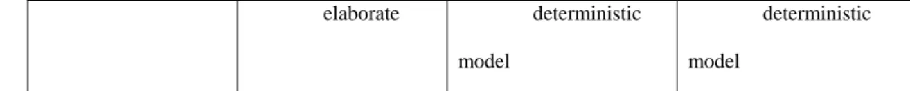
(27) 596. As a consequence, there is no unique solution to detect trends in groundwater. 597. quality across widely differing catchments. The choice of the method for trend. 598. detection and extrapolation should firstly be made on the basis of the system under. 599. study, and secondly on the available resources and goals (Table 5). A classical. 600. statistical approach may serve for an initial survey to detect changes in groundwater. 601. quality. In simple single-porosity groundwater bodies with access to monitoring wells. 602. with short screens groundwater dating is an excellent tool for the demonstration of. 603. trend reversal. In complex dual-porosity systems, a transfer function approach is. 604. better suited for preliminary trend detection. Transfer functions may be used for trend. 605. extrapolation, but only with great care to ensure that the predicted trends are within. 606. the range of the observations. In these systems, groundwater dating may serve to. 607. confirm the hydrological functioning and transfer times of the system. Deterministic. 608. groundwater modeling should be applied in areas with high ecological, economical or. 609. sustainability importance.. 610. Regardless of the complexity of the model used, being transfer functions or. 611. deterministic models, trend detection and extrapolation is always associated with. 612. uncertainty. This means that groundwater quality monitoring should remain a priority.. 613. Additional data will improve the detection of trends and increase the knowledge of the. 614. functioning of the groundwater system. Better understanding of the system, possibly. 615. derived from deterministic modeling, can in turn provide feedback for the. 616. optimization of the groundwater quality monitoring networks.. 617 618. [Table 5]. 619. 27.

(28) 620. 7.. Acknowledgements. 621. This work was supported by the European Union FP6 Integrated Project. 622. AquaTerra (Project no. GOCE 505428) under the thematic priority “sustainable. 623. development, global change and ecosystems”.. 624 625. 8.. References. 626 627. Almasri, M.N. and Ghabayen, S.M.S., 2008. Analysis of nitrate contamination of. 628. Gaza Coastal Aquifer, Palestine. Journal of Hydrologic Engineering, 13(3):. 629. 132-140.. 630. Almasri, M.N. and Kaluarachchi, J.J., 2004. Assessment and management of long-. 631. term nitrate pollution of ground water in agriculture-dominated watersheds.. 632. Journal of Hydrology, 295(1-4): 225-245.. 633. Almasri, M.N. and Kaluarachchi, J.J., 2005. Modular neural networks to predict the. 634. nitrate distribution in ground water using the on-ground nitrogen loading and. 635. recharge data. Environmental Modelling & Software, 20(7): 851-871.. 636 637 638. Almasri, M.N. and Kaluarachchi, J.J., 2007. Modeling nitrate contamination of groundwater in agricultural watersheds. Journal of Hydrology, 343(3-4): 211. Amraoui, N., Surdyk, N. and Dubus, I.G., 2008. Physically-deterministic. 639. determination and extrapolation of time trends at in the Brévilles' catchment. 640. (Chpt. 4). In: H.P. Broers and A. Visser (Editors), Report which describes the. 641. physically-deterministic determination and extrapolation of time trends at. 642. selected test locations in Dutch part of the Meuse basin, the Brévilles. 643. catchment and the Geer catchment (Deliverable T2.10), Utrecht, The. 644. Netherlands.. 28.

(29) 645. Baran, N., Dubus, I.G., Morvan, X., Normand, M., Gutierrez, A. and Mouvet, C.,. 646. 2004. Climatic and land use data for the Brévilles experimental catchment. 647. (Chpt. 4). In: H.P. Broers and A. Visser (Editors), Report with documentation. 648. of reconstructed land use around test sites (Deliverable T2.2), Utrecht, The. 649. Netherlands.. 650. Batlle-Aguilar, J. and Brouyère, S., 2004. Spatial dataset for Meuse BE (Chpt. 3). In:. 651. H.P. Broers and A. Visser (Editors), Documented spatial data set containing. 652. the subdivision of the basins into groundwater systems and subsystems, the. 653. selected locations per subsystem and a description of these sites, available data. 654. and projected additional measurements and equipment (Deliverable T2.1),. 655. Utrecht, The Netherlands.. 656. Batlle-Aguilar, J., Orban, P. and Brouyère, S., 2005. Point by Point Statistical Trend. 657. Analysis and Extrapoled Time Trends at Test Sites in the Meuse BE (Chpt. 3).. 658. In: H.P. Broers and A. Visser (Editors), Report on extrapolated time trends at. 659. test sites (Deliverable T2.4), Utrecht, The Netherlands.. 660. Batlle-Aguilar, J., Orban, P., Dassargues, A. and Brouyère, S., 2007. Identification of. 661. groundwater quality trends in a chalk aquifer threatened by intensive. 662. agriculture in Belgium. Hydrogeology Journal, 15(8): 1615.. 663. Bohlke, J.K., Wanty, R., Tuttle, M., Delin, G. and Landon, M., 2002. Denitrification. 664. in the recharge area and discharge area of a transient agricultural nitrate plume. 665. in a glacial outwash sand aquifer, Minnesota. Water Resources Research,. 666. 38(7): -.. 667 668. Broers, H.P., 2002. Strategies for regional groundwater quality monitoring. PhD Thesis, Utrecht University, Utrecht, 231 pp.. 29.

(30) 669. Broers, H.P., 2004. The spatial distribution of groundwater age for different. 670. geohydrological situations in the Netherlands: implications for groundwater. 671. quality monitoring at the regional scale. Journal of Hydrology, 299(1-2): 84-. 672. 106.. 673. Broers, H.P., Rozemeijer, J., Van Der Aa, M., Van Der Grift, B. and Buijs, E.A.,. 674. 2005. Groundwater quality trend detection at the regional scale: Effects of. 675. spatial and temporal variability, IAHS-AISH Publication, pp. 50-60.. 676 677 678. Broers, H.P. and van der Grift, B., 2004. Regional monitoring of temporal changes in groundwater quality. Journal of Hydrology, 296(1-4): 192-220. Broers, H.P., Visser, A., Dubus, I.G., Baran, N., Morvan, X., Normand, M., Gutierrez,. 679. A., Mouvet, C., Batlle-Aguilar, J., Brouyère, S., Orban, P., Dautrebande, S.,. 680. Sohier, C., Korcz, M., Bronder, J., Dlugosz, J. and Odrzywolek, M., 2004a.. 681. Report with documentation of reconstructed land use around test sites. 682. (Deliverable T2.2), Utrecht, The Netherlands.. 683. Broers, H.P., Visser, A. and Van der Grift, B., 2004b. Land use history and the. 684. chemical load of recharging groundwater in agricultural recharge areas of the. 685. Dutch Meuse basin (Chpt. 2). In: H.P. Broers and A. Visser (Editors), Report. 686. with documentation of reconstructed land use around test sites (Deliverable. 687. T2.2), Utrecht, The Netherlands.. 688. Burow, K., Dubrovsky, N. and Shelton, J., 2007. Temporal trends in concentrations of. 689. DBCP and nitrate in groundwater in the eastern San Joaquin Valley,. 690. California, USA. Hydrogeology Journal, 15(5): 991-1007.. 691. Busenberg, E. and Plummer, L.N., 1992. Use of Chlorofluorocarbons (CCl3F and. 692. CCl2F2) as Hydrologic Tracers and Age-Dating Tools - the Alluvium and. 30.

(31) 693. Terrace System of Central Oklahoma. Water Resources Research, 28(9):. 694. 2257-2283.. 695. Busenberg, E. and Plummer, L.N., 2000. Dating young groundwater with sulfur. 696. hexafluoride: Natural and anthropogenic sources of sulfur hexafluoride. Water. 697. Resources Research, 36(10): 3011-3030.. 698 699 700 701. Carabin, G. and Dassargues, A., 1999. Modeling Groundwater with Ocean and River Interaction. Water Resources Research, 35(8): 2347-2358. Carr, J.R., 1995. Numerical analysis for the geological sciences. Prentice Hall, Englewood Cliffs, NJ, 592 pp.. 702. Dassargues, A. and Monjoie, A., 1993. The chalk in Belgium. In: R.A. Downing, M.. 703. Price and G.P. Jones (Editors), The hydrogeology of the chalk of North-West. 704. Europe. Oxford Science Publ., Oxford, pp. 153 - 269.. 705. Daughney, C.J. and Reeves, R.R., 2005. Definition of hydrochemical facies in the. 706. New Zealand National Groundwater Monitoring Programme. Journal of. 707. Hydrology New Zealand, 44(2): 105-130.. 708. Daughney, C.J. and Reeves, R.R., 2006. Analysis of temporal trends in New Zealand's. 709. groundwater quality based on data from the National Groundwater Monitoring. 710. Programme. Journal of Hydrology New Zealand, 45(1): 41-62.. 711. Di, H.J., Cameron, K.C., Bidwell, V.J., Morgan, M.J. and Hanson, C., 2005. A pilot. 712. regional scale model of land use impacts on groundwater quality. Management. 713. of Environmental Quality, 16(3): 220-234.. 714. Dubus, I.G., Baran, N., Gutierrez, A., Guyonnet, D. and Mouvet, C., 2004. Spatial. 715. dataset for Brévilles (Chpt. 4). In: H.P. Broers and A. Visser (Editors),. 716. Documented spatial data set containing the subdivision of the basins into. 717. groundwater systems and subsystems, the selected locations per subsystem. 31.

(32) 718. and a description of these sites, available data and projected additional. 719. measurements and equipment (Deliverable T2.1), Utrecht, The Netherlands.. 720. Dubus, I.G., Gutierrez, A., Mouvet, C. and Baran, N., 2005. Subsoil input data. 721. prepared for groundwater and reactive transport modelling in the French. 722. Brévilles catchment. In: H.P. Broers and A. Visser (Editors), Subsoil input. 723. data prepared for groundwater and reactive transport modelling in Dutch part. 724. of the Meuse basin (Deliverable T2.5), Utrecht, The Netherlands.. 725 726 727 728 729. EU, 2006. Directive 2006/118/EC on the Protection of Groundwater against Pollution and Deterioration. Gardner, K.K. and Vogel, R.M., 2005. Predicting ground water nitrate concentration from land use. Ground Water, 43(3): 343-352. Gourcy, L., Dubus, I.G., Baran, N., Mouvet, C. and Gutierrez, A., 2005. First. 730. investigations into the use of environmental tracers for age dating at the. 731. Brévilles experimental catchment (Chpt. 4). In: H.P. Broers and A. Visser. 732. (Editors), Report on concentration-depth, concentration-time and time-depth. 733. profiles in the Meuse basin and the Brévilles catchment (Deliverable T2.3),. 734. Utrecht, The Netherlands.. 735. Harbaugh, A.W., Banta, E.R., Hill, M.C. and McDonald, M.G., 2000. MODFLOW-. 736. 2000, the U.S. Geological Survey modular ground-water model - User guide. 737. to modularization concepts and the Ground-Water Flow Process. USGS Open-. 738. File Report 00-92.. 739 740. Harris, J., Loftis, J.C. and Montgomery, R.H., 1987. Statistical Methods for Characterizing Ground-Water Quality. Ground Water, 25(2): 185-193.. 741. Helsel, D.R. and Hirsch, R.M., 1995. Statistical methods in water resources. Studies. 742. in environmental science, 49. Elsevier, Amsterdam, the Netherlands, 529 pp.. 32.

(33) 743. Hirsch, R.M., Alexander, R.B. and Smith, R.A., 1991. Selection of methods for the. 744. detection and estimation of trends in water quality. Water Resources Research,. 745. 27(5): 803-813.. 746 747 748 749 750. Hirsch, R.M., Slack, J.R. and Smith, R.A., 1982. Techniques of trend analysis for monthly water quality data. Water Resources Research, 18(1): 107-121. Hudak, P.F., 2000. Regional trends in nitrate content of Texas groundwater. Journal of Hydrology, 228(1-2): 37-47. Jiang, Y., Yuan, D., Xie, S., Li, L., Zhang, G. and He, R., 2006. Groundwater quality. 751. and land use change in a typical karst agricultural region: A case study of. 752. Xiaojiang watershed, Yunnan. Journal of Geographical Sciences, 16(4): 405-. 753. 414.. 754 755 756. Kendall, M.G., 1948. Rank Correlation Methods. Charles Griffin & Company, London. Korcz, M., Dlugosz, J. and Bronder, J., 2007. Report which describes the approach. 757. used for inter well trend comparison with application to the Bille-Krückau. 758. watershed and comparison with classical multivariate analyses (Deliverable. 759. T2.9).. 760. Korcz, M., Slowikowski, D., J.Bronder and Dlugosz, J., 2004. Spatial dataset for Elbe. 761. Basin (Chpt. 5). In: H.P. Broers and A. Visser (Editors), Documented spatial. 762. data set containing the subdivision of the basins into groundwater systems and. 763. subsystems, the selected locations per subsystem and a description of these. 764. sites, available data and projected additional measurements and equipment. 765. (Deliverable T2.1), Utrecht, The Netherlands.. 766 767. Laier, T., 2004. Nitrate monitoring and CFC-age dating of shallow groundwaters - an attempt to check the effect of restricted use of fertilizers. In: L. Razowska-. 33.

(34) 768. Jaworek and A. Sadurski (Editors), Nitrate in Groundwaters, IAH Selected. 769. papers on hydrogeology. A.A. Balkema, Leiden, the Netherlands, pp. 247-258.. 770. Lapworth, D.J., Gooddy, D.C., Stuart, M.E., Chilton, P.J., Cachandt, G., Knapp, M.. 771. and Bishop, S., 2006. Pesticides in groundwater: some observations on. 772. temporal and spatial trends. Water and Environment Journal, 20(2): 55-64.. 773. Lee, J.Y., Yi, M.J., Yoo, Y.K., Ahn, K.H., Kim, G.B. and Won, J.H., 2007. A review. 774. of the National Groundwater Monitoring Network in Korea. Hydrological. 775. Processes, 21(7): 907-919.. 776 777 778 779. Loftis, J.C., 1996. Trends in groundwater quality. Hydrological Processes, 10: 335355. Loftis, J.C., Taylor, C.H. and Chapman, P.L., 1991. Multivariate tests for trend in water quality. Water Resources Research, 27(7): 1419-1429.. 780. MacDonald, A.M., Darling, W.G., Ball, D.F. and Oster, H., 2003. Identifying trends. 781. in groundwater quality using residence time indicators: an example from the. 782. Permian aquifer of Dumfries, Scotland. Hydrogeology Journal, 11(4): 504-. 783. 517.. 784. Mann, H.B., 1945. Nonparametric tests against trend. Econimetrica, 13: 245-259.. 785. Mouvet, C., Albrechtsen, H.J., Baran, N., Chen, T., Clausen, L., Darsy, C.,. 786. Desbionne, S., Douguet, J.M., Dubus, I.G., Esposito, A., Fialkiewicz, W.,. 787. Gutierrez, A., Haverkamp, R., Herbst, M., Howles, D., Jarvis, N.J., Jørgensen,. 788. P.R., Larsbo, M., Meiwirth, K., Mermoud, A., Morvan, X., Normand, B., O,. 789. M.C., Ritsema, C., Roessle, S., Roulier, S., Soutter, M., Stenemo, F., Thiéry,. 790. D., Trevisan, M., Vachaud, G., Vereecken, H. and Vischetti, C., 2004.. 791. PEGASE. Pesticides in European Groundwaters: detailed study of. 792. representative aquifers and simulation of possible evolution scenarios. In: I.G.. 34.

(35) 793. Dubus and C. Mouvet (Editors), Final Report of the European Project #EVK1-. 794. CT1990-00028. BRGM/RP-52897-FR.. 795. Orban, P., Batlle-Aguilar, J. and Brouyère, S., 2005. Input data sets for groundwater. 796. and transport modelling in the Geer basin (Chpt. 3). In: H.P. Broers and A.. 797. Visser (Editors), Subsoil input data prepared for groundwater and reactive. 798. transport modelling in Dutch part of the Meuse basin (Deliverable T2.5),. 799. Utrecht, The Netherlands.. 800. Orban, P., Batlle-Aguilar, J., Goderniaux, P. and Brouyère, S., 2008. Physically-. 801. deterministic determination and extrapolation of time trends in the Geer. 802. catchment (Chpt. 3). In: H.P. Broers and A. Visser (Editors), Report which. 803. describes the physically-deterministic determination and extrapolation of time. 804. trends at selected test locations in Dutch part of the Meuse basin, the Brévilles. 805. catchment and the Geer catchment (Deliverable T2.10), Utrecht, The. 806. Netherlands.. 807. Orban, P. and Brouyère, S., 2007. Report with results of groundwater flow and. 808. reactive transport modelling in the Geer catchment (Chpt. 3). In: H.P. Broers. 809. and A. Visser (Editors), Report with results of groundwater flow and reactive. 810. transport modelling at selected test locations in Dutch part of the Meuse basin,. 811. the Brévilles' catchment and the Geer catchment (Deliverable T2.8), Utrecht,. 812. The Netherlands.. 813. Pinault, J.-L., Guyonnet, D., Dubus, I.G., Baran, N., Gutierrez, A. and Mouvet, C.,. 814. 2005. Conventional and innovative approaches to trends analysis: a case study. 815. for the Brévilles catchment (Chpt. 4). In: H.P. Broers and A. Visser (Editors),. 816. Report on extrapolated time trends at test sites (Deliverable T2.4), Utrecht,. 817. The Netherlands.. 35.

(36) 818. Pinault, J.L., 2001. Manuel utilisateur de TEMPO: logiciel de traitement et de. 819. modélisation des séries temporelles en hydrogéologie et en hydrogéochemie.. 820. Projet Modhydro. Rap. BRGM/RP-51459, BRGM, Orleans.. 821. Pinault, J.L. and Dubus, I.G., 2008. Stationary and non-stationary autoregressive. 822. processes with external inputs for predicting trends in water quality. Journal of. 823. Contaminant Hydrology, In Press, Accepted Manuscript.. 824. Refsgaard, J.C., Thorsen, M., Jensen, J.B., Kleeschulte, S. and Hansen, S., 1999.. 825. Large scale modelling of groundwater contamination from nitrate leaching.. 826. Journal of Hydrology, 221(3-4): 117-140.. 827. Reynolds-Vargas, J., Fraile-Merino, J. and Hirata, R., 2006. Trends in nitrate. 828. concentrations and determination of its origin using stable isotopes (18O and. 829. 15N) in groundwater of the western Central Valley, Costa Rica. Ambio, 35(5):. 830. 229-236.. 831. Ritter, A., Munoz-Carpena, R., Bosch, D.D., Schaffer, B. and Potter, T.L., 2007.. 832. Agricultural land use and hydrology affect variability of shallow groundwater. 833. nitrate concentration in South Florida. Hydrological Processes, 21(18): 2464-. 834. 2473.. 835. Schlosser, P., Stute, M., Dorr, H., Sonntag, C. and Munnich, K.O., 1988. Tritium/3He. 836. Dating of Shallow Groundwater. Earth and Planetary Science Letters, 89(3-4):. 837. 353-362.. 838 839 840 841. Shapiro, S.S. and Francia, R.S., 1972. An approximate analysis of variance test for normality. Journal of the American Statistical Association, 67(337): 215-216. Shapiro, S.S. and Wilk, M.B., 1965. An analysis of variance test for normality (complete samples). Biometrika, 52: 591-611.. 36.

(37) 842. Stuart, M.E., Chilton, P.J., Kinniburgh, D.G. and Cooper, D.M., 2007. Screening for. 843. long-term trends in groundwater nitrate monitoring data. Quarterly Journal of. 844. Engineering Geology and Hydrogeology, 40(4): 361-376.. 845. Tesoriero, A.J., Spruill, T.B., Mew, H.E., Farrell, K.M. and Harden, S.L., 2005.. 846. Nitrogen transport and transformations in a coastal plain watershed: Influence. 847. of geomorphology on flow paths and residence times. Water Resources. 848. Research, 41(2): -.. 849. Van der Grift, B. and Griffioen, J., 2008. Modelling assessment of regional. 850. groundwater contamination due to historic smelter emissions of heavy metals.. 851. Journal of Contaminant Hydrology, 96(1-4): 48-68.. 852. Van der Grift, B. and Van Beek, C.G.E.M., 1996. Hardness of abstracted. 853. groundwater: indicative predictions (in Dutch), Kiwa, Nieuwegein, the. 854. Netherlands.. 855. Van Maanen, J.M.S., de Vaan, M.A.J., Veldstra, A.W.F. and Hendrix, W.P.A.M.,. 856. 2001. Pesticides and nitrate in groundwater and rainwater in The Province of. 857. Limburg in the Netherlands. Environmental Monitoring and Assessment,. 858. 72(1): 95-114.. 859 860 861. Visser, A., Broers, H.P. and Bierkens, M.F.P., 2007a. Dating degassed groundwater with 3H/3He. Water Resources Research, 43(10): WR10434. Visser, A., Broers, H.P. and Van der Grift, B., 2004. Spatial dataset for Meuse NL. 862. (Chpt. 2). In: H.P. Broers and A. Visser (Editors), Documented spatial data set. 863. containing the subdivision of the basins into groundwater systems and. 864. subsystems, the selected locations per subsystem and a description of these. 865. sites, available data and projected additional measurements and equipment. 866. (Deliverable T2.1), Utrecht, The Netherlands.. 37.

(38) 867. Visser, A., Broers, H.P. and Van der Grift, B., 2005a. Concentration-depth,. 868. concentration–time and groundwater age-depth profiles in groundwater in dry. 869. agricultural areas of the lower Meuse basin NL (Chpt. 2). In: H.P. Broers and. 870. A. Visser (Editors), Report on concentration-depth, concentration-time and. 871. time-depth profiles in the Meuse basin and the Brévilles catchment. 872. (Deliverable T2.3), Utrecht, The Netherlands.. 873. Visser, A., Broers, H.P. and Van der Grift, B., 2005b. Demonstrating trend reversal. 874. using tritium-helium age scaling: results for the Dutch Meuse subcatchment. 875. (Chpt. 2). In: H.P. Broers and A. Visser (Editors), Report on extrapolated time. 876. trends at test sites (Deliverable T2.4), Utrecht, The Netherlands.. 877. Visser, A., Broers, H.P., Van der Grift, B. and Bierkens, M.F.P., 2007b.. 878. Demonstrating Trend Reversal of Groundwater Quality in Relation to Time of. 879. Recharge determined by 3H/3He. Environmental Pollution, 148 (3): 797-807.. 880. Visser, A., Van der Grift, B. and Broers, H.P., 2005c. Subsoil input data prepared for. 881. groundwater and reactive transport modelling in Dutch part of the Meuse basin. 882. (Chpt. 2). In: H.P. Broers and A. Visser (Editors), Subsoil input data prepared. 883. for groundwater and reactive transport modelling in Dutch part of the Meuse. 884. basin (Deliverable T2.5), Utrecht, The Netherlands.. 885. Visser, A., Van der Grift, B. and Broers, H.P., 2006. Subsoil input data prepared for. 886. groundwater and reactive transport modelling in Dutch part of the Meuse basin. 887. (Chpt. 2). In: H.P. Broers and A. Visser (Editors), Input data sets and short. 888. report describing the subsoil input data for groundwater and reactive transport. 889. modelling at test locations in Dutch part of the Meuse basin, the Brévilles'. 890. catchment and the Geer catchment (Deliverable T2.5), Utrecht, The. 891. Netherlands.. 38.

(39) 892. Visser, A., Van der Grift, B., Heerdink, R. and Broers, H.P., 2008. Physically-. 893. deterministic determination and extrapolation of time trends at selected test. 894. locations in Dutch part of the Meuse basin (Chpt. 2). In: H.P. Broers and A.. 895. Visser (Editors), Report which describes the physically-deterministic. 896. determination and extrapolation of time trends at selected test locations in. 897. Dutch part of the Meuse basin, the Brévilles catchment and the Geer. 898. catchment (Deliverable T2.10), Utrecht, The Netherlands.. 899. Vogel, J.C., 1967. Investigation of groundwater flow with radiocarbon, IAEA. 900. Symposium on Isotopes in Hydrology. IAEA, Vienna, pp. 355-369.. 901. Wassenaar, L.I., Hendry, M.J. and Harrington, N., 2006. Decadal geochemical and. 902. isotopic trends for nitrate in a transboundary aquifer and implications for. 903. agricultural beneficial management practices. Environmental Science and. 904. Technology, 40(15): 4626-4632.. 905. Xu, Y., Baker, L.A. and Johnson, P.C., 2007. Trends in Ground Water Nitrate. 906. Contamination in the Phoenix, Arizona Region. Ground Water Monitoring &. 907. Remediation, 27(2): 49-56.. 908. Yue, S., Pilon, P. and Cavadias, G., 2002. Power of the Mann-Kendall and. 909. Spearman's rho tests for detecting monotonic trends in hydrological series.. 910. Journal of Hydrology, 259(1-4): 254-271.. 911. Zheng, C. and Wang, P.P., 1999. MT3DMS: A modular three-dimensional. 912. multispecies transport model for simulation of advection, dispersion, and. 913. chemical reactions of contaminants in groundwater systems. Documentation. 914. and user's guide, Department of Geological Sciences, University of Alabama,. 915. Alabama.. 916. 39.

(40) 917 918. 40.

(41) 919. Tables. 920 Sub-basin. Hydrogeological characteristics. Spatial scale. Contaminants. Methods used. Dutch part of Meuse basin (Brabant/Kemp en). Unconsolidated Plesitocence deposits; fine to medium coarse sands, loam. 5000/500 km2. Nitrate, sulfate, Ni, Cu, Zn, Cd. Statistical, groundwater dating and deterministic modelling. WallonyHesbaye. Cretaceous chalk, fissured, dual porosity aquifer. 440 km2. Nitrate. Wallony-Pays de Herve. Cretaceous chalk and sands, fissured. 285 km. Nitrate. Statistical, groundwater dating and deterministic modelling Statistical. WallonyNéblon Wallony-Meuse alluvial plain. Carboniferous limestone, folded karstified Unconsolidated deposits; gravels, sands and clays. 65 km. Nitrate. Statistical. 125 km2. Nitrate. Statistical. Brévilles. Lutecian limestone over Cuise sands, limestone fissured. 2.5 km2. Pesticides (Atrazine and DEA). Elbe basin. unconsolidated glacial deposits of sand and gravel. 1300 km2. Nitrate. Transfer functions and deterministic modelling Statistical and groundwater dating. Walloon part of Meuse basin. 921 922 923. Table 1: Characteristics of the test sites. Groundwater body Geer basin Pays of Herve Néblon basin Alluvial plain. 924 925 926. Percent of significant trends 57.7% 66.6% 83.3% 68.4% Table 2. Summary of trend tests results for each groundwater body in the Walloon part of the Meuse basin. Prerequisite. NO3 -. K 40%  11% . Number of downward trends 0 2 1 15. Number of upward trends 15 6 4 11. OXC CL 20%  20%  33% , 44%  11%  Table 3: Percentage of significant trends detected in Bille-Krückau data set. shallow deep. 927 928 929. Number of nitrate points 26 12 6 38. Al 0% -. Purely statistical approaches. Transfer function approaches. Age dating. Collection of monitoring data in the field. Collection of monitoring data in the field. Collection of monitoring data in the field +. 41. Deterministic modelling with poor fit to the data Collection of monitoring data in the field +. SUMCAT 20%  11% . Deterministic modelling with good fit to the data Collection of monitoring data in the field +.

(42) 930 931 932. + Collection of information on the input flux (rainfall, and either inputs or land use). information on the evolution of the input function + analysis of tracers in samples. 1 (surveys if not already available purchasing of met data) Functional understanding of the system (identification of the key factors and understanding of their influence). 10. Associated cost magnitude (on top of the data collection effort) Understanding of the system?. None. Extrapolation potential Potential universality to all systems. Poor. Good. Good. Potentially. Potentially. Limited, only applies to homogeneous systems. +. No understanding of the system. Functional understanding of the system. Heavy effort in collection of additional information (other piezometers, pumping and tracer tests, geophysics, soil mapping) 100 (geophysics, additional piezometers, soil mapping) Detailed data on the system, but lack of overall understanding of the functioning of the system (exemplified by the lack of fit of the deterministic model) Poor. Heavy effort in collection of additional information (other piezometers, pumping and tracer tests, geophysics, soil mapping) 100 (geophysics, additional piezometers, soil mapping) Potential detailed understanding of the system under study. Good. Potentially. Potentially. Potential for ++ + operational use Knowledge ++ + ++ +++ about the functioning of the system Table 4: Summary table comparing the strengths and weaknesses of each of the trends analysis methodologies Groundwater system. Trend detection. simple. complex. preliminary. Statistics. Statistics. elaborate. Groundwater. Transfer. dating Trend extrapolation. preliminary. functions Statistical. Transfer. methods for short term. functions for short term. extrapolation. extrapolation. 42.

(43) elaborate. deterministic model. 933 934 935. deterministic model. Table 5: Recommended preliminary and elaborate methods for trend detection and extrapolation in simple and complex groundwater systems.. 936. 43.

(44) 937. Figures. 938 939. N surpluses Wielom. (N-surpluses). kg/( ha a) N. Schleswig-Holstein, Korcz, IETU. Source: CEA. Wallony Belgium, Brouyere, ULg. 940 941. Visser et al, EnvPol, 2007. Figure 1: History of N-fertilizer application in NL, Belgium, Germany . ! . !. OSTER. ELLINGSTEDT. Treia. OLDERSBEK. Strande/Neubulk. F. . ! ! .. BREKENDORF. . !. Kl. Bennebek !.. Felm. . !. ! . . !. ! .. Kropp. . !. Garding Beo. Schneidershoop. ALT BENNEBEK. . !. . !. FARGEM. KLAMP/WENTORF MARIENWARDER. NORDERHEISTEDT. Langwedel. . !. BREIHOLZ-OST. ! . . !. TIEBENSEE. ! .. . !. . !. ! .. . !. Riepsdorf. ! .. . !. Westerborstel. Barmissen. KROGASPE . !. NINDORF. ! .. Krumstedt . !. . !. NIENBUTTEL. . !. Kesdorf. Wapelfeld Nienjahn. St. Michaelisdon. !! . .. Goennebek. . !. . !. . ! . ! Trappenkamp !. BLUNK. . !. ROHLSTORF. HOHENFIERT. WAHLSTEDT. HAGEN. ! .. Nordbuttel. ! .. ! .. . !. Bockhorn. . ! . !. Lentforden Heidmoor. !! . . . !. . .! !! .. ! .. . !. . !. HOLM. . !. MP Basic Net. . !. Labenz. ! .. . !. ! .. NEUHORST. . ! . ! Hamburg. Sachsenwald. FITZEN. . !. GWB CODE. ! .. Wohltorf. El 15. GULZOW . !. El 16. . !. Lutau. El 17. El-b 0. 5 000. 10 000. 20 000. 30 000. 40 000. Meters. Figure 4: Location of selected groundwater bodies. 942. Figure 2: Location of test sites within Europe and detailed map of test sites. 44. KITTLITZ. Grosshansdorf WITZHAVE. Bille-Kruckau GW bodies. County boundaries. Kittlitz Hin ! .. RELLINGEN. WEDEL Elbe Basin in Shleswig Holstein. ! . . !. ! .. Hasloh. ! . . !. MP Trend Net. SIEBENBSUMEN. Tangstedter Forst Ellerhoop. ! .. AHRENLOHE. . !. Leezen-Nord. BARMSTEDT. Tornesch!.!.. HEIDGRABEN. Seestermuhe. . !. ! . . !. HORST. Legend. Schlutup. . !. Brokreihe. ! .. . !. Langenlehsten Heide.

(45) 943. DATASET Shapiro-Wilks test (<50 values) Shapiro-Francia test (>50 values). Normality. Non-Normality. Linear regression. Mann-Kendall test. Trend. Slope regression. 944 945 946 947. 948 949 950 951 952. No trend. Trend. No trend. Kendall's Slope. Figure 3: A three step procedure is adopted for trend analysis of nitrate concentrations in the selected groundwater bodies: 1) normal/non-normal distribution data; 2) trend detection; 3) trend estimation.. Figure 4: The concentrations of a conservative chemical indicator (OXC) sampled from the shallow (8m) and deep (24m) screens of observation wells 108 and 122 (right) plotted at the recharge year of the sampled groundwater (left). The result is the concentration - recharge year relationship, from which a clear trend can be observed that was not visible in the individual time series.. 45.