Monitoring cork and holm oak woodlands with Google Earth Engine

(1)

HAL Id: dumas-01950823

https://dumas.ccsd.cnrs.fr/dumas-01950823

Submitted on 11 Dec 2018

HAL is a multi-disciplinary open access

archive for the deposit and dissemination of sci-entific research documents, whether they are pub-lished or not. The documents may come from teaching and research institutions in France or abroad, or from public or private research centers.

L’archive ouverte pluridisciplinaire HAL, est destinée au dépôt et à la diffusion de documents scientifiques de niveau recherche, publiés ou non, émanant des établissements d’enseignement et de recherche français ou étrangers, des laboratoires publics ou privés.

Distributed under a Creative Commons Attribution - NonCommercial - NoDerivatives| 4.0 International License

Monitoring cork and holm oak woodlands with Google

Earth Engine

Valentine Aubard

To cite this version:

Valentine Aubard. Monitoring cork and holm oak woodlands with Google Earth Engine. Life Sciences [q-bio]. 2018. �dumas-01950823�

(2)

Monitoring cork and holm oak woodlands

with Google Earth Engine

Par : Valentine AUBARD

Soutenu à Rennes le 13 septembre 2018

Devant le jury composé de :

Présidents : Hervé Nicolas, Samuel Corgne Maîtres de stage : João Manual Das Neves Silva, Joana Amaral Paulo

Enseignant référent : Hervé Nicolas

Autres membres du jury (Nom, Qualité) : Rodéric Béra, Maitre de Conférence Hervé Squividant, Ingénieur

Les analyses et les conclusions de ce travail d'étudiant n'engagent que la responsabilité de son auteur et non celle d’AGROCAMPUS OUEST

AGROCAMPUS OUEST CFR Angers CFR Rennes

Année universitaire : 2017-2018 Spécialité : Ingénieur agronome et territorial (Vetagro-Sup)

Spécialisation (et option éventuelle) : Télédétection et environnement (TELENVI, Agrocampus-Ouest)

Mémoire de Fin d'Études

d’Ingénieur de l’Institut Supérieur des Sciences agronomiques, agroalimentaires, horticoles et du paysage

de Master de l’Institut Supérieur des Sciences agronomiques, agroalimentaires, horticoles et du paysage

d'un autre établissement (étudiant arrivé en M2)

Ce document est soumis aux conditions d’utilisation

«Paternité-Pas d'Utilisation Commerciale-Pas de Modification 4.0 France»

(3)

(4)

(5)

(6)

Abstract

Oak woodlands are being documented to be declining in southern Europe. In order to verify and quantify this phenomenon, 34-year trends of the Normalized Difference Vegetation Index (NDVI) were calculated and mapped at 30-meter pixel scale for all cork oak (Quercus suber) and holm oak (Quercus

ilex) areas of continental Portugal.

NDVI is considered a good proxy to monitor trees health and productivity along years. Landsat 5, 7 and 8 imagery from 1984 to 2017 were used to derive a long-term NDVI time series. MODIS 250-m spatial resolution NDVI product was used to compare values for the period after 2000. All imagery were freely available and treatable on Google Earth Engine. NDVI values of Landsat 5 and 8 were adjusted to Landsat 7 values. Only July and August NDVI were used to minimize the spectral contribution of understorey vegetation and its phenological variability, thus focusing on the tree layer. Signs and significance of trends were calculated by Mann-Kendall (MK) and contextual MK tests, and their slopes using Theil-Sen (TS) estimator. The methodological approach was first tested on six cork oaks stands. Linear models revealed the effect of annual cumulated precipitation and debarking on NDVI variations. All trends were found significant. A Pettitt test showed significant change-points around the year 2000. At country scale, a spatio-temporal trend analysis was performed on stable cover areas of holm and cork oak. Thirty percent of woodlands area presents declining trends, mainly located in Centro region, and interior and littoral of Alentejo.

Keywords: Quercus suber L., Quercus ilex L., Montado, Time series, Normalized Difference Vegetation

(7)

Résumé

Introduction/Etat de l’art – De nombreux articles scientifiques décrivent le déclin des forêts de

chênes du Sud de l’Europe. Les chênes lièges (Quercus suber L.) et chênes verts (Quercus ilex L.) couvrent un tiers du Portugal continental, et ont une grande valeur économique, sociale et environnementale pour le territoire. Les chênes lièges sont surtout exploités pour le liège, matériel utilisé pour les bouchons de bouteilles et l’isolation, dû à son élasticité et sa faible perméabilité. Il est extrait de l’arbre adulte tous les 9 ans ou plus. Le Portugal possède 50% du marché mondial. Les chênes verts produisent de riches glands utilisés pour l’alimentation animale, en plus de protéger le bétail du froid en hiver et du soleil en été. Le potentiel de la télédétection et de la plateforme Google Earth Engine (GEE) ont été utilisés pour établir les tendances de productivité de ces deux espèces sur une longue période et pour tout un/le pays. GEE permet de manipuler gratuitement en ligne des données rasters et vecteurs du monde entier. Cette étude permet d’évaluer ses performances pour le traitement d’image appliqué au suivi des parcelles forestières. L’indice de végétation par différence normalisé NDVI (Normalized Difference Vegetation Index) a déjà prouvé être un bon proxy pour suivre la production et la santé des forêts méditerranéennes de chênes. Il sera utilisé à une échelle spatiale adaptée, bien plus précise que les précédentes études.

Objectifs et Plan – L’objectif principal de ce travail était de quantifier spatialement le déclin

annoncé des chênes et de délivrer une carte des tendances sur 34 ans de toutes les parcelles de chênes lièges et de chênes verts du Portugal continental. Le second objectif était de comprendre les principales variables expliquant les variations de NDVI au fil des ans. Pour ce faire, la première partie du travail a été d’établir une méthodologie pour extraire des tendances de séries temporelles, de l’appliquer et de la valider à l’échelle de la parcelle, en suivant les NDVI de six peuplements de chênes lièges portugais, et de trouver des variables explicatives pour ces variations. La seconde partie fut d’appliquer cette méthode pour cartographier les tendances de NDVI de ces deux espèces pour toute l’aire du Portugal continental.

Partie 1 – Matériel et méthodes. Six parcelles de chêne liège de 1 hectare furent sélectionnées

pour leur diversité de production de liège, leur densité, leur localisation, leur sol et végétation de sous-étage. Les images SR Tier 1 des capteurs Landsat -5, -7 et -8 furent utilisées pour calculer les NDVI à une résolution spatiale de 30 mètres, entre 1984 et 2017, tous les 16 jours. Une fonction Fmask leurs a été appliquée pour ôter nuages et ombres. La version 6 du produit MODIS Terra Vegetation Indices, qui fournit les NDVI à 250 mètres de résolution fut utilisée pour comparer les résultats. Un ajustement des valeurs de NDVI entre les différents capteurs Landsat était nécessaire dû aux différences de sensibilité de longueur d’onde des bandes utilisées. Des équations spécifiques à chaque parcelle furent établies et leur fiabilité comparée aux équations proposées de la littérature. Seule une moyenne des valeurs de NDVI des mois de Juillet et Août a été utilisée pour l’analyse, période pendant laquelle les valeurs de NDVI de la végétation de sous-étage sont minimales, tandis que celles des arbres ne varient que peu pendant l’année. Les tendances d’évolution des valeurs de NDVI au cours du temps (en année) étant supposées monotones, le test non-paramétrique de Mann-Kendall et l’estimateur de Theil-Sen furent utilisés pour estimer la significativité, le signe des tendances et leur vitesse d’évolution (pente). Un test de Pettitt a été appliqué pour détecter d’éventuelles ruptures de tendance. Des modèles linéaires multiples furent établis pour tester l’effet sur les valeurs de NDVI de la quantité de précipitations, cumulées par an ou par saison, et de l’extraction du liège.

Partie 1 – Résultats et discussion. Pour ajuster les valeurs de NDVI entre les différents capteurs

Landsat, l’équation proposée par Ju et al. (2016) entre Landsat-5 et -7 se révéla la meilleure et utilisable à large échelle. Entre Landsat-7 et -8, seules les équations établies pour chaque site d’étude semblèrent corriger efficacement la différence, et furent retenues pour les analyses de la Partie 1, mais les valeurs de NDVI de Landsat-8 ne furent pas utilisées pour l’ensemble du Portugal. La comparaison

(8)

des NDVI des capteurs Landsat et MODIS sur la période 2000-2017 a permis de valider ces choix. La quantité annuelle de précipitations (entre Août de l’année précédente et Juillet) révéla être corrélée positivement et significativement à la moyenne de NDVI de Juillet-Août, les quantités de précipitations au printemps et en été étant les plus déterminantes. Cela concorde avec les relations déjà mises en évidence entre précipitations et productivité des arbres (en quantité de liège). L’extraction du liège (entre Juin et Août) l’année précédente semble avoir un impact significatif négatif sur la moyenne de NDVI de Juillet-Aout. L’extraction la même année n’eut pas d’effet significatif. Cela laisse supposer que le chêne va d’abord investir son énergie dans la production de nouveau liège, nécessaire à sa régulation hydrique et sa protection contre les feux, au printemps suivant, plutôt que dans la production de nouvelles feuilles, qui peut être différée en automne. Les tendances obtenues pour les six sites d’étude ont été significatives et leurs signes et taux cohérents avec la production de liège connue pour chaque parcelle. Deux sites présentent des tendances négatives, qui peuvent indiquer une diminution de la densité de la parcelle ou un stress des arbres de plus en plus important au fil du temps, avec répercussion sur le feuillage. Des ruptures de tendances significatives ont été trouvées pour chaque parcelle, oscillant entre 1996 et 2005, ce qui suggère une rupture de tendance dans les variables influençant les valeurs de NDVI des chênes lièges et chênes verts autour de l’an 2000.

Partie 2 – Matériel et méthodes. Seuls furent utilisés les peuplements de chênes lièges et chênes

verts gardant la même classe d’occupation du sol au cours du temps, déterminés grâce aux cartes d’utilisation et d’occupation des sols portugaises (Carta de Uso e Ocupação do Solo (COS)) de 1995, 2007, 2010 et 2015. La classification très précise des COS fut simplifiée en cinq classes : forêts de chênes lièges, forêts de chênes verts, systèmes agroforestiers (SAF) de chênes lièges, SAF de chênes verts et SAF où coexistent les deux espèces. Un masque des aires ayant subi un ou plusieurs feux de forêts entre 1984 et 2017 fut ensuite appliqué. Suivant les résultats de la Partie 1, seuls les moyennes de NDVI de Juillet-Août des capteurs Landsat-5 (valeurs ajustées selon l’équation proposée par Ju et

al. (2016)) et Landsat-7 furent utilisées pour établir les séries temporelles par pixel de 1984 à 2017. Le

test de Mann-Kendall a été utilisé pour obtenir le signe et la significativité des tendances, ainsi que le test contextuel de Mann-Kendall, prenant en compte les pixels voisins pour estimer la significativité. L’estimateur de Theil-Sen fut ensuite appliqué pour obtenir la vitesse d’évolution (pente).

Partie 2 – Résultats et discussion. La carte des tendances significatives et non-significatives des

peuplements de chênes lièges et chênes verts fut obtenue pour le territoire continental portugais, excepté les aires inférieures à l’aire unitaire minimale des COS (1ha). De même, les feux de forêts d’aire inférieure à 5ha ne furent pas masqués. Aucune COS n’existe avant 1995 pour assurer que les classes d’occupation des parcelles retenues n’évoluèrent pas entre 1984 et 1995. Le type de production et la législation portugaise actuelle assurent néanmoins une grande stabilité de ce couvert dans le temps. Cette carte indique des zones en déclin notamment dans la région Centro, le littoral et l’intérieur de l’Alentejo. Sur toute l’aire traitée, trente pour cent des tendances significatives sont décroissantes, indiquant la mort de certains arbres (diminuant la densité de la canopée) ou une diminution de plus en plus drastique de la capacité photosynthétique des arbres chaque été. Par classe, les SAF de chênes lièges donnèrent le pourcentage de tendances significatives négatives le plus élevé ; les SAF de chênes verts donnèrent le plus bas. Cette différence peut s’expliquer par la plus grande capacité d’adaptation des chênes verts à des conditions xérophytiques, notamment dans les SAF, de faible densité. Un abandon progressif des SAF de chênes lièges pourrait également expliquer ce résultat. Un élargissement de la carte a été fait autour de chaque site étudié en Partie 1 pour visualiser les différences entre les résultats des tests de Mann-Kendall et contextuel de Mann-Kendall, globalement similaires. Les résultats des Parties 1 et 2 furent cohérents, et les élargissements mirent en évidence l’importante corrélation spatiale mais également la grande variabilité des tendances de pixels proches. Cette variabilité pourrait être expliquée seulement par une étude exhaustive des sites, prenant en compte divers facteurs comme la pente, l’exposition, la texture et la lithologie des sols, l’âge des arbres, les potentielles maladies et la gestion humaine (de la végétation de sous-étage, du pâturage et

(9)

de l’extraction du liège). Bien évidemment, une étude aussi précise peut difficilement être réalisée à l’échelle d’un pays.

Conclusion – Ce travail a montré les avantages et les faiblesses de Google Earth Engine pour le suivi

forestier. La méthodologie adoptée pour ce travail a permis d’établir une carte détaillée des tendances sur 34 ans de l’indice NDVI, vu comme un proxy de la productivité, pour deux espèces d’arbres, à l’échelle d’un pays entier. Pour un suivi à haute échelle de résolution spatiale sur un site de taille raisonnable, cette méthodologie peut être améliorée en prenant en compte le pourcentage de couvert de la canopée, et la composition de la végétation de sous-étage au cours du temps, et ainsi évaluer la part du couvert arboré dans les valeurs de NDVI. Cette méthode peut être reproduite et adaptée à d’autres indices de végétation, d’autres espèces, d’autres lieux et d’autres problématiques. Les résultats donnent un signal d’alerte et pointent les besoins d’une meilleure compréhension du déclin observé, ainsi que de la recherche de solutions dans un contexte de réchauffement climatique.

(10)

Acknowledgements

Special thanks to my supervisors, Joana Amaral Paulo, João Manuel Das Neves Silva and to their respective teams, for their guidance, ideas, advises, and continual support. This research was carried out in the Centro de Estudos Florestais (Forest Research Centre) of the Instituto Superior de Agronomia (School of Agriculture), University of Lisbon.

Thanks to my referent teacher Hervé Nicolas, professor of Agrocampus-Ouest school, for his support and advises. Acknowledgements are also due to my various teachers of Vetagro-Sup, Agrocampus-Ouest and the University of Rennes 2 for sharing their knowledge and for their patience. At last, thanks to the Auvergne-Rhône-Alpes region and to the Erasmus+ program for their financial support which made this six-month internship possible.

(11)

(12)

List of Figures

Figure 1: Localization of the six cork oak stands in Portugal. ... 3

Figure 2: Cumulated precipitation from August to next July (mm) per study-site, from the closest climate stations. ... 5

Figure 3: Methodology to adjust the NDVI values derived from different Landsat sensors. ... 7

Figure 4: Comparison of adjusted-Landsat and MODIS NDVI variation along years. ... 13

Figure 5: Mean cork production in millimetres per year per plot function of 34-year NDVI trends (from 1984 to 2017). ... 17

Figure 6: Landsat NDVI summer means per year for each study-site. ... 18

Figure 7: Masks of constant land cover classes (left) and burned areas (right)... 21

Figure 8: Mann-Kendall test results - signs and significance... 23

Figure 9: Frequency histogram of significant and not significant slope (left), and significant slopes only (right), for the 5 classes of land use. ... 24

Figure 10: Theil-Sen slopes and Mann-Kendall significance. ... 25

Figure 11: Theil Sen slopes and Mann-Kendall significance maps per land cover class. ... 26

Figure 12: Theil-Sen slopes around the six study-sites, with Kendall and Contextual Mann-Kendall significance. ... 28

List of Tables

Table 1: Characteristics of the six stands. ... 4

Table 2: Most recent debarking dates for the six study-sites. ... 5

Table 3: Image collections used in Google Earth Engine. ... 6

Table 4: Bibliographic equations of adjustment. ... 8

Table 5: Determined site-specific NDVI adjustment equations between Landsat sensors. ... 8

Table 6: Percentages of absolute differences in means (%D means) and medians (%D medians) between Landsat-5 and Landsat-7 NDVI. ... 12

Table 7: Percentages of absolute differences in means (%D means) and medians (%D medians) between Landsat-8 and Landsat-7 NDVI. ... 12

Table 8: Parameter estimates for the NDVIt model (Equation 2). ... 15

Table 11 : Pearson’s correlation and Mann-Kendall Tau. ... 16

Table 12: Linear trend (L) and Theil Sen estimator (TS) comparison. ... 17

Table 13: Results of Pettitt change-point test per study-site for Landsat time-series (1984- 2017). ... 19

Table 14: Five classes used to summarise the classification of the COS. ... 21

Table 15: Area and percentage of total area of Mann-Kendall map results. ... 22

Table 16: Means of Theil-Sen slope per class. ... 24

(13)

List of Appendix

Appendix 1: Fmask function coded in Google Earth Engine following pixel quality values. ... I Appendix 2: Comparison of bands of Landsat and MODIS sensors. ... II Appendix 3: Comparison of NDVI values for cork oaks, herbaceous and shrubs along years. ... III Appendix 4: Normal Q-Q plots for the six study-site, for Landsat-5, -7 and -8 derived-NDVI raw-values.

... IV Appendix 5: Boxplots to compare the accuracy of NDVI adjustment equations between Landsat-5, -7 and -8 sensors. ... V Appendix 6: Comparison of adjusted and not-adjusted Landsat -5 and -8 NDVIs. ... VI Appendix 7: Matches between the classes kept (Code) and the original classes of the Portuguese land use and land cover maps (Carta de Uso e Ocupação do Solo (COS)) for 1995, 2007-2010 and 2015 classifications. ... VII Appendix 8: Evolution of area covered per each class of land cover, and comparison with the amount of constant areas of each class. ... VIII Appendix 9: Enlargement of the masks of constant land cover classes and burned areas. ... IX Appendix 10: Enlargement of Theil Sen slopes and Mann-Kendall significance maps per land cover class.

... XI Appendix 11: Frequency histograms of all slopes and significant slopes values for each land cover class.

(14)

Introduction

An important decline of oaks species have been noticed in the last decades in Portugal due to various possible factors such as land management, especially livestock grazing (Godinho et al., 2016), difficult access to ground water in summer in hilltops and shallow soils (Costa et al., 2010), climate change (Kim et al., 2017), associated to pests and diseases (Brasier et al., 1993; Romero et al., 2007). This decline has been observed in several ecosystem variables such has the number of trees per hectare (Costa et al., 2009; Silva J. S., 2007), tree regeneration, tree canopy cover (Paulo et al., 2015a) or cork growth (Paulo et al., 2017).

Woodlands of cork oak (Quercus suber L.) and holm oak (Quercus ilex L.) cover one third of woodland areas of the continental territory of Portugal, mostly as an artificial extensive silvopastoral system called montado (ICNF, 2013). They have an important value for Portugal’s economy, society and environment, providing various ecosystem services as landscape and tourism hotspots, reducing fire risk and soil erosion, increasing carbon sequestration and key-habitats for rare and endemic species (Moreno et al., 2017; Da Silva et al., 2009).

Cork oaks are exploited mainly for cork, but under the typical silvopastoral management system acorns are also a valuable product for animal feeding. Cork is one of the most valuable product of non-wood forest exploitation worldwide, having remarkable mechanics properties as low permeability to liquids and gases, rot-proof and important elasticity (Pereira, 2007). It is used mainly for bottle stoppers, although isolation uses can also be applied. Also, an emerging clothing market and other products have been expanding. Portugal is the main producer in the world, with 50% of the global market, and the sector contribute to 3% of the gross domestic product of the country, providing a considerable amount of job positions specially on rural areas. Workable cork, the third stripping since the first two don’t have a proper properties, is extracted from adult trees – from 50 to 150 years old, sometimes the double – with a minimal gap of 9 years between each debarking according to the current national legislation in Portugal.

Holm oaks produce characteristic acorns that are used to feed livestock, in particular black pigs which are associated with these stands and produce premium meat, or for culinary purposes. The trees are also good shelter either in winter, against frost, either in summer against heat and sun exposure. Holm oak wood is known to be extremely calorific and is traditionally used as firewood. Also, before the development of fossil fuel, holm wood was for this reason valued for charcoal production (Rigueiro-Rodríguez et al., 2008; Moreno et al., 2017).

In order to evaluate the long-term productivity trends of those two species for a whole country, the potentialities of remote sensing and of the new open access platform Google Earth Engine (GEE) were considered to be exploited. GEE gives free access to thousands of geographic information system features (vector and raster) from all over the world. The JavaScript code editor allows to manipulate them online, without downloading, and to save images or table results on a stockage platform. Therefore, this study will be an opportunity to evaluate to what extent Google Earth Engine is adapted to the needs and purpose of image processing with the goal of forest monitoring.

A strong correlation exists between wood, leaves and seed production of North American oak species and the Normalized Difference Vegetation Index (NDVI) at 1-km of spatial resolution, from the National Oceanic and Atmospheric Administration Advanced Very High Resolution Radiometer (NOAA/AVHRR) satellite (Wang et al., 2004). The Moderate Resolution Imaging Spectroradiometer

(17)

2 (MODIS) NDVI at 250-m of resolution was also proved to be an efficient indicators of forest biomass growth and dieback in Mediterranean holm oak forests (Ogaya et al., 2015). In this study, NDVI is used as a proxy of cork and acorn productivity and of the global health of holm oak and cork oak stands.

The first objective of this work was to spatially quantify oaks decline and to deliver a map of 34-year NDVI trends for all cork oak and holm oak areas of continental Portugal. The spatial scale of this analysis had to meet the needs of plot monitoring. The second objective was to understand the main factors explaining oaks NDVI variations along years.

The work was divided in two parts: 1) establishing a methodology to extract times series trends at plot scale, following the NDVI evolution of six Portuguese cork oak woodlands, and finding explanatory variables for NDVI variations; 2) applying this method to map spatio-temporal NDVI trends of cork and holm oak areas for the whole territory of continental Portugal.

(18)

3

Part 1: NDVI trends at plot scale

1. Material and methods

1.1 Study-site characterization

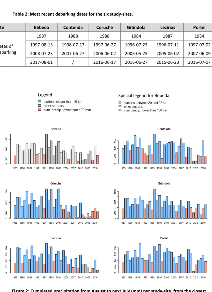
Six pure cork oak stands were chosen throughout Portugal (Figure 1), contrasting in their distance to the sea, density, understorey and cork production (Table 1). Their cork productivity is being followed since the 90s by the group Forest Ecosystem Management Under Global Change (ForChange) of the Forest Research Centre (CEF) of the Instituto Superior de Agronomia (ISA) in Lisbon. The dates of debarking of each stand are described in Table 2, and cumulated precipitation per year, from 1983 to 2017, in

Figure 2. Portugal has a Mediterranean

climate with a very defined dry season in summer and mild temperature in winter.

The area of each plot is around 1 ha, thus can be fitted 11 Landsat pixels or 0.16 MODIS pixels. The areas were defined by a circular buffer of 57 m² around the center of the plot (a polygon with 24 vertices) of exactly 1.0085 ha. The center was selected in order to get the most homogeneous canopy cover possible.

1.2 Satellite image characterization

Images from four sensors were used for this study following two objectives: 1) making the longest period available time series at the most precise spatial scale possible; 2) validating the results with images taken from a unique sensor to avoid sensor bias.

First, 30-m pixel with a 16-day cycle Landsat images from three sensors were chosen (Table 3) to create a time series of 34 years, between 1984 and 2017. GEE provide Top of Atmosphere (TOA) and Surface Reflectance (SR) images from Landsat-4, -5, -7 and -8. Only the already atmospherically compensated SR images were used. Landsat-4 images were ignored since the collection contains only 64 images for all Portugal between 1988 and 1993, period already covered by Landsat-5 images. For Landsat-5, -7 and -8, only the first category of data ‘Tier 1’ (T1) produced by the United States Geological Survey (USGS) was used, since it meets geometric and radiometric quality requirements.

Figure 1: Localization of the six cork oak stands in Portugal.

(19)

4

Table 1: Characteristics of the six stands.

* mean for each plot, according to the 30-m pixel Landsat Tree Cover Continuous Fields layer for 2010, which gives a percentage of the vertically projected area of vegetation (including leaves, stems, branches, etc.) of woody plants greater than 5 meters in height (GEE Image Collection ID: GLCF/GLS_TCC). ** from measure of rings thickness after boiling, following the methodology used by Paulo and Tomé (2010), the mean was calculated for each stand from samples of 23 to 36 trees, for two debarking periods (a total of 17 to 22 years).

*** soil group classification of IUSS working group WRB (2006).

Site Bêbeda Contenda Coruche Grândola Lezírias Portel

Longitude

(EPSG:4326) -8.781102 -7.103938 -8.335581 -8.438551 -8.855579 -7.634190

Latitude (EPSG:4326) 38.000741 38.075716 39.139173 38.102245 38.815475 38.253932

Tree age (in 2010) Even-aged, around 70 years old

Uneven-aged (natural regeneration), more

than 100 years old

Even-aged, around 60 years old

Uneven-aged (natural regeneration), more

than 100 years old

Even-aged, around 70 years old Even-aged, 90-100 years old Estimated canopy cover (percentage in 2010) * 13.1 8.8 18.8 7.3 23.8 12.8

Mean cork thickness

(mm.tree-1_.year-1_{) **} 3.43 2.53 4.15 3.06 3.30 2.64

Understorey Medium shrubs and herbs

Medium shrubs and

herbs Pasture, cow grazing

Pasture, sheep grazing

Abundant herbaceous

A few shrubs and herbs, sheep and cow

grazing

FAO soil group *** Arenosoils Leptosoils Podzols Arenosoils and

(20)

5

Table 2: Most recent debarking dates for the six study-sites.

Site Bêbeda Contenda Coruche Grândola Lezírias Portel

Dates of debarking 1987 1988 1988 1984 1987 1984 1997-08-13 1998-07-17 1997-06-27 1996-07-27 1996-07-11 1997-07-02 2008-07-23 2007-06-27 2006-06-02 2006-05-25 2005-06-02 2007-06-09 2017-08-01 / 2016-06-17 2016-06-27 2015-06-23 2016-07-07

Special legend for Bêbeda: Legend:

Figure 2: Cumulated precipitation from August to next July (mm) per study-site, from the closest climate stations.

(21)

6 The Fmask function (Zhu and Woodcock, 2012) was implemented in GEE to remove clouds and shadows from Landsat images, using the quality of pixel band (pixel_qa). The attributes of the pixel_qa band and the function used in GEE are presented in the Appendix 1. All images of Landsat-7 taken after May 31, 2003 contain "SLC-off gaps" due to the failure of the Scan Line Corrector (SLC) of the sensor. On GEE, the values of the missing pixels are informed as 'NA’ values. No interpolation to fill those gaps was made. Second, version 6 of the MODIS Terra Vegetation Indices (Table 3) provides bands of NDVI and EVI at 250-m scale every 16 days, already fully corrected, including cloud-masked. This dataset was chosen to validate Landsat results between 2000 and 2017.

Table 3: Image collections used in Google Earth Engine.

Sensor Range of available

dates* Time scale Spatial scale GEE Image Collection ID used

Landsat-5 TM 1984-01-01 -

2012-05-05 16-day cycle 30x30 m LANDSAT/LT05/C01/T1_SR

Landsat-7 ETM+ 1999-01-01 -

2018-05-31 16-day cycle 30x30 m LANDSAT/LE07/C01/T1_SR

Landsat-8 OLI 2013-04-11 -

2018-06-14 16-day cycle 30x30 m LANDSAT/LC08/C01/T1_SR

MODIS Terra V6 Vegetation Indices

2000-02-18 -

2018-05-25 16-day cycle 250x250 m MODIS/006/MOD13Q1 *on 2018-06-28: new images take as much as one month to be evaluated.

1.3 NDVI and adjustment between Landsat sensors

The Normalized Difference Vegetation Index (NDVI, Equation 1) (Rouse et al., 1974) exploits the highly reflectance of the vegetation in the near infrared (NIR) region and its strong chlorophyll absorption in the visible region.

NDVI = (NIR - Red) / (NIR + Red) Equation 1

where NIR is Landsat SR individual Near Infrared channel, respectively band 4 for Landsat-5 and -7, band 5 for Landsat-8 and Red is Landsat SR individual Red channel, respectively band 3 for Landsat-5 and -7, band 4 for Landsat-8.

(22)

7 A difference is expected between the values of the vegetation index regarding the differences of bands wavelength sensibility presented in Appendix 2 between Landsat-5, -7 and -8. To establish trends, an adjustment between the three Landsat sensors-derived NDVI is thus essential. Some linear relations have already been established for the United States (She et al., 2015, Roy et al., 2016), Canada (Ju et al., 2016) and Northern Europe (Steven et al., 2003) (Table 4). The first step of this study was to select the best relations for Portugal. The accuracy of the equations selected from literature was compared with site-specific equations made for each plot (Table 5). Site-specific equations have been calculated for each plot adjusting Landsat-5 and Landsat-8 NDVI values to Landsat-7 values. The methodology adopted, schematically explained on the Figure 3 below, was inspired by the tandem images cross-calibration of Ju et al., 2016. For each site, NDVI values were extracted from 1984-01-01 to 2017-12-31 for each pixel intersecting the buffer area. Site-specific relations were assumed linear, with an intercept equal to zero, the literature equation intercepts being very small when not null (Table

4). Only images values from different sensors separated by a time-gap of 8 days (minimum gap possible

in Portugal) were used, backward and forward.

Source: Valentine AUBARD, 2018

(23)

8

Table 4: Bibliographic equations of adjustment.

Reference X a b

Steven et al., 2003 L5 1.0210 -0.0010

Ju et al., 2016 L5 1.0370 0

Roy et al., 2016 L8 0.9589 0.0029 She et al., 2015** L8 1.0204 -0.0112 ** equation for evergreen forests NDVI in summer.

Equations are under the form Y = a * X + b, where Y is the Landsat-7 derived-NDVI and X either Landsat-5 (L5) or Landsat-7 (L7) NDVI.

Table 5: Determined site-specific NDVI adjustment equations between Landsat sensors.

Site X Backward images Forward images Total images Available pixels a R² Bêbeda L5 52 76 128 1165 1.0205 0.9866 Contenda L5 17335 14212 31547 6445 1.0101 0.9754 Coruche L5 123 124 247 1984 1.0124 0.9922 Grândola L5 26175 21395 47570 5191 1.0109 0.9821 Lezírias L5 65 63 128 1362 1.0039 0.9878 Portel L5 9095 8457 17552 5863 1.0345 0.9772 Bêbeda L8 879 888 1767 2526 0.8907 0.9931 Contenda L8 9361 9975 19336 5904 0.8976 0.9832 Coruche L8 145 142 287 2333 0.9050 0.9915 Grândola L8 32856 34359 67215 5098 0.8793 0.9862 Lezírias L8 79 78 157 1731 0.8974 0.9893 Portel L8 10540 11387 21927 6061 0.8600 0.9841

Equations are under the form Y = a * X (considering b = 0), where Y is the Landsat-7 derived-NDVI and X either Landsat-5 (L5) or Landsat-8 (L8) NDVI. The number of images on Day -8 and Day +8 are quiet equilibrated. Less clear images are available for the sites close to the sea (frequent clouds). However, the total number of available pixels is always greater than 1000.

(24)

9 1.4 Months used to establish trends

One-hectare NDVI averages were extracted for each site between 1984-01-01 and 2017-12-31. Previous studies run in Machoqueira do Grou (Coruche) about the reflectance of trees, herbaceous and shrubs along years (Cerasoli et al., 2016) have proven that cork oaks NDVI response was close to steady through the year, while the herbaceous absorbance shows large phenological variations, being the lowest in the driest-summer months of July and August (Appendix 3.a). Basically, the herbaceous vegetation dries by lack of water in summer while the trees, due to deeper root systems, access to groundwater reserves all over the year. This result is less reliable for shrubs, mainly depending on the species (Appendix 3.b).

To reduce understorey influence and establish the trends of each site focusing on the tree layer (cork or holm oak), only July-August mean-NDVI value was used in each year. The absence of outliers was previously checked for each plot using July-August NDVI values interquartile range (range between 25th_{and 75}th_{percentile), to introduce no error in the mean. Focusing on summer months has also the} double advantage of reducing the area of tree shadows on the images (due to high solar elevation angle) and creating an equally-distant-in-time dataset. Making the hypothesis that the trends were monotonic, the non-parametric Mann-Kendall test (Mann, 1945; Kendall, 1975) was used to obtain the strength and direction of the trends, and a value of the rate of change (slope) was given by Theil-Sen robust linear estimator (Theil, 1950; Sen, 1968). The null hypothesis of Mann-Kendall test is that there is no monotonic trend in the series, alternative hypothesis are the existence of a positive or negative monotonic trend. A Pettitt test (Pettitt, 1979) was also applied to approximate the date of a potential change-point. Those tests were run in R software using packages stats version 3.4.2 (R Core Team, 2017), zyp version 0.10-1 (Bronaugh and Werner, 2013) and trend version 1.1.0 (Pohlert, 2018).

1.5 Effect of precipitation and debarking on trees NDVI

Based on current knowledge and scientific literature, two variables were supposed to have a noticeable effect on NDVI variations: groundwater and debarking. As a matter of fact, one of the strategies of the tree to respond to hydric stress, e. g. caused by lack of groundwater or by debarking (traditionally made between June and August), is to regulate evapotranspiration by decreasing foliage extent (Paulo et al., 2017; Mendes et al., 2016; Natividade, 1950). The annual cumulated waterfall can be used as a proxy to estimate the variations of groundwater resources (Ferreira et al., 2007). A positive relation between annual precipitation rate and July-August trees NDVI is thus expected, while a negative effect of debarking could be observed. These variables were used for the definition of multiple linear regressions that were fitted using stats package from R software version 3.4.2 (R Core Team, 2017). Normality of distribution, absence of multicollinearity, and homoscedasticity of the dataset were checked.

The annual cumulated precipitation (cum_precip) was calculated using the nearest meteorological stations data from each study-site (Figure 2), available at the network SNIRH – Sistema Nacional de Informação de Recursos Hídricos (https://snirh.apambiente.pt/), from Augustt-1 to Julyt to be coherent with NDVIt, mean of Julyt and Augustt months values. The previous summer NDVIt-1 was included in the equation, since the NDVI series is supposed to be temporally correlated (Equation 2). To separate the effects of the precipitation for each season of the year, a second model was tested (Equation 3) that includes separate variables for spring (precip_spring), summer (precip_summer), autumn (precip_autumn) and winter (precip_winter). Trees are debarked with a minimum of 9-year time-gap that is sometimes extended for 10 or 11 year’s intervals. Taking advantage of the knowledge of extract

(25)

10 debarking years on each of the six plots considered, it was possible to test the hypothesis that the debarking operation has an impact on the NDVI of the same year or of the next year. Presence of debarking on the same year (debarkt) or the year before NDVI measurement (debark(t-1)) was added in Equation 4.

NDVIt ~ β0 + β1 * yeart + β2 * NDVI(t-1) + β3 * cum_precip + ε Equation 2

where NDVIt is the annual Julyt-Augustt mean of Landsat-derived NDVI, yeart is the year of NDVIt measurement, NDVI(t-1) is the NDVI of the previous year, cum_precip is the cumulated precipitation from Augustt-1 (of yeart-1) to Julyt (of yeart), β0 is the intercept and β1, β2, β3 are the correlation coefficients associated with the independent parameters and ε is the random error component.

NDVIt ~ β0’ +β1’ * yeart + β2’ * NDVI(t-1) + β3’ * precip_autumn + β4’ * precip_winter + β5’ * precip_spring

+ β6’ * precip_summer + ε’ Equation 3

where NDVIt is the annual Julyt-Augustt mean of Landsat-derived NDVI, yeart is the year of NDVIt measurement, NDVI(t-1) is the NDVI of the previous year, precip_autumn, precip_winter, precip_spring, precip_summer the annual cumulated precipitation per season, respectively from Septembert-1 to Novembert-1, Decembert-1 to Februaryt, Marcht to Mayt, Junet to Augustt, β0’, the intercept and β1’,…, β6’ the correlation coefficients associated with the independent parameters and ε’ the random error component.

NDVIt ~ β0’’ + β1’’ * yeart + β2’’ * NDVI(t-1) + β3’’ * cum_precip

+ β4’’ * debarkt + β5’’ * debark(t-1) + ε’’ Equation 4

where NDVIt is the annual Julyt-Augustt mean of Landsat-derived NDVI, yeart is the year of NDVIt measurement, NDVI(t-1) is the NDVI of the previous year, cum_precip the cumulated precipitation from August(t-1) to Julyt, debarkt, the existence of a debarking on the same year, debark(t-1) the existence of a debarking on the previous year, β0’’, the intercept and β1’’, …,β5’’ the correlation coefficients associated with the independent parameters and ε’’ the random error component.

(26)

11

2. Results and Discussion

2.1 Best NDVI-adjustment equations

To evaluate the performances of bibliographic and site-specific equations (respectively in Table 4 and Table 5), for adjusting the three Landsat sensors NDVI values, samples were taken from the periods shared by two sensors: from 1999-01-01 to 2012-05-05 for Landsat-5 and -7 derived NDVIs; from 2013-04-11 to 2017-12-31 for Landsat-7 and -8 derived NDVIs. Since the populations do not follow a normal distribution (Appendix 4) and time-series observations are supposed auto-correlated, it was chosen to compare the percentages of differences between means and medians of Landsat-7 sample and the corresponding Landsat-5 and Landsat-8 samples not-adjusted and adjusted with each equation (respectively Table 6 and Table 7). Boxplots were plotted for a visual approach (Appendix 5).

To adjust Landsat-8 NDVIs according to Landsat-7 values, no bibliographic equation fitted well. The site-specific correction is accurate enough to be used for each site. For studying a large area at a 30m-pixel scale (e.g. mainland Portugal), however, this methodology is for now too demanding in terms of processing to be applied on GEE. The simplest and safest solution is thus to not used Landsat-8 values, since 7 reaches the end of the period chosen. To adjust 5 NDVI according to Landsat-7, the observed differences seem far less important than between Landsat-8 and Landsat-7 NDVI. The equation given on the works of Ju et al. (2016) gives the closest values. This equation will be considered good enough to be used at small and large study areas.

2.2 Evolution of NDVI values along years

Landsat-5 and Landsat-8 had been adjusted for each site with its specific equation. Not-adjusted NDVI values of 8 are always greater than 7 values on equivalent dates, while Landsat-5 values are always lower. Adjusted values are similar to Landsat-7 NDVI for the same period (Appendix

6). The evolution of NDVI values have been compared graphically between Landsat and MODIS sensors

(Figure 4). The values are close and their evolution is identical along years. Every plot presents a large intra-annual variation of NDVI due to vegetation phenology. The maximum are reached in December-January and the minimum in July-August. The difference between those two values depends of the percentage of canopy cover (Häusler et al., 2016). Those observations support the hypothesis that NDVI cycles exist for every composition of understorey and every percentage of canopy cover.

2.3 Explaining NDVI variations with precipitation and debarking

Fitting the multilinear regression with all of the stands simultaneously decrease the effect of the variable yeart (Equation 2, Table 8) and lets appear the high correlation between NDVI values of one year and the next (NDVIt-1 and NDVIt). As expected, annual precipitation amounts are positively correlated to NDVI values: more precipitation, higher NDVI. The works of Caritat et al. (2000) and Faias

et al. (2018) already showed annual cork rings thickness is positively correlated with annual

precipitation. These results thus confirm NDVI is a good proxy for following cork oaks (cork) productivity. Yeart, being a significant component, suggests other variables are needed to fully explain NDVI values, such as other pedo-climatological variables or human practices (debarking, shrubs management, grazing).

(27)

12

Table 6: Percentages of absolute differences in means (%D means) and medians (%D medians) between Landsat-5 and Landsat-7 NDVI.

Site Type L5 Raw Data L5 Steven et al., 2003 L5 Ju et al., 2016 L5 Site specific

Bêbeda %D means -5.275 -3.492 -1.770 -3.329 Contenda %D means -8.785 -7.085 -5.410 -7.868 Coruche %D means -3.499 -1.644 0.072 -2.303 Grândola %D means -9.750 -8.074 -6.411 -8.764 Lezírias % Dmeans -1.707 0.177 1.930 -1.324 Portel % Dmeans -7.582 -5.880 -4.162 -4.391

Average mean error (%) -6.099 -4.392 -3.292 -4.663

Bêbeda %D medians -5.010 -3.224 -1.496 -3.060 Contenda %D medians -13.134 -11.540 -9.920 -12.260 Coruche %D medians -3.293 -1.435 0.285 -2.094 Grândola %D medians -10.412 -8.772 -7.097 -9.433 Lezírias %D medians -1.815 0.066 1.818 -1.432 Portel %D medians -6.667 -4.963 -3.213 -3.444

Average median error (%) -6.722 -5.000 -3.971 -5.287

Table 7: Percentages of absolute differences in means (%D means) and medians (%D medians) between Landsat-8 and Landsat-7 NDVI.

Site Type L8 Raw Data L8 Roy et al., 2016 L8 She et al., 2015 L8 Site specific

Bêbeda %D means 12.874 8.839 12.843 0.539 Contenda %D means 11.640 7.707 11.385 0.207 Coruche %D means 9.218 5.207 9.602 1.159 Grândola %D means 12.712 8.689 12.659 0.888 Lezírias %D means 9.452 5.437 9.819 1.783 Portel %D means 19.949 15.789 19.422 3.156

Average mean error (%) 12.641 8.611 12.622 1.289

Bêbeda %D medians 14.681 10.584 14.637 2.148 Contenda %D medians 13.299 9.384 12.746 1.696 Coruche %D medians 9.885 5.846 10.281 0.555 Grândola %D medians 17.209 13.066 16.996 3.066 Lezírias %D medians 9.983 5.946 10.363 1.306 Portel %D medians 24.588 20.337 23.771 7.145

(28)

13

(29)

14 In the second model (Equation 3), where cumulated precipitation is decomposed per seasons, adjusted-R-squared is slightly better (Table 9). Precip_autumn and precip_winter are not significantly explaining NDVI values of July-August, there is supposedly no hydric stress on those seasons. Of course, it can also be a bias from taking only summer NDVI values. The main impacts on NDVI are found in spring, when the these oaks produce new leaves, and in summer, when the temperatures cause an important need of water, making the trees very sensible to the variations of precipitation during this season. These results are in line with the ones obtained by Caritat et al. (2000). It is also in June and July than cork oaks produce the most quantity of cork under favourable climate conditions (Costa et

al., 2003). One of the tree’s strategies in case of hydric stress is to lower transpiration by losing leaves,

which will therefore decrease NDVI values, allowing to follow health and productivity.

Debarking of yeart has no significant effect on summer NDVIt (Equation 4, Table 10). A possible explanation for this is that since the cork is removed between June and August (Table 2), when the new leaves of the year are already well developed, the operation will not have an important impact on the NDVI values recorded. Supporting this result is the fact that a minor effect of the debarking in the leaves may be observed, in some trees, during a short and varying period of time averaging 15 days after debarking, when the trees are recovering from loss of water by transpiration of the stem (Natividade, 1950; Correia et al., 1992; and Werner and Correia, 1996), which is a too short reaction to be observed by a 2-month-mean of NDVI.

Results also show a significant negative effect of the debarking (debarkt-1) on next year NDVIt. An hypothesis would thus be that the trees, in the spring after the debarking operation, allocate resources and photo-assimilated compounds to produce a new cork layer that allows to increase the protection from fire and loss of water during summer, delaying and/or decreasing leaf production to a later season such as autumn or even to the following year. This hypothesis is supported by the observations of Vaz

et al. (2010) or Costa e Silva et al. (2015), that observed this event respectively after a dry summer and

a dry winter.

2.4 Significant NDVI trends for the six study-sites

The Table 11 below presents the results for the Pearson’s correlation and the Mann-Kendall test, using the annual means of July-August Landsat-5 adjusted, -7 and -8 adjusted-derived NDVI. Pearson’s null hypothesis is that there is no correlation in the population, and its alternative hypothesis is that there is correlation (here, between NDVI values and the time in years). Its results is between -1 and 1, with 1 being a total positive correlation, 0 an absence of correlation and -1 being a total negative correlation. The significance of the correlation is given by a two-sided p-value and the limits of its confidence interval (conf. Int.). Mann-Kendall test is non-parametric and resistant to outliers, gives the significance and sign of a supposed monotonic trend in a time series (here July-August NDVI values for 34 years). The sign of its result, tau, indicates the sign of the trend. Tau has a value between -1 and 1, which follows a normal distribution for times series longer than 30 years, so the value can be used directly to determine the significance of the trend (values between -1.96 and 1.96). Its two-sided p-value give the same result.

For Landsat, the Pearson’s confidence intervals show how far from 0 all the correlations are. The p-values, similar for Pearson and Mann-Kendall tests, are highly significant, asserting the existence of strongly significant trends for each site. The sign of Pearson’s correlation and Kendall’s tau match. Two study-sites, Contenda and Portel, have a decreasing trend of NDVI between 1984 and 2017. They are actually the two plots with lower cork production per tree (Table 1). The other stands present a positive trend.

(30)

15

Table 8: Parameter estimates for the NDVIt model (Equation 2).

Estimate Std. Error t-value p-value

Intercept -1.716e+00 8.482e-01 -2.023 0.04447

yeart 8.694e-04 4.222e-04 2.059 0.04081

NDVI(t-1) 8.697e-01 3.758e-02 23.141 < 2e-16

cum_precip 5.562e-05 1.705e-05 3.261 0.00131

Multiple R-squared: 0.7396 Adjusted R-squared: 0.7356.

Table 9: Parameter estimates for the NDVIt model (Equation 3).

Intercept -2.191e+00 8.179e-01 -2.679 0.008029

yeart 1.098e-03 4.072e-04 2.698 0.007607

NDVI(t-1) 8.854e-01 3.606e-02 24.554 <2e-16 precip_autumn -2.584e-05 3.320e-05 -0.778 0.437469

precip_winter 4.467e-05 2.690e-05 1.660 0.098518

precip_spring 1.955e-04 5.218e-05 3.746 0.000238

precip_summer 4.919e-04 1.184e-04 4.153 4.94e-05

Multiple R-squared: 0.769 Adjusted R-squared: 0.7617

Table 10: Parameter estimates for the NDVIt model (Equation 4).

Multiple R-squared: 0.747 Adjusted R-squared: 0.741

Intercept -1.850e+00 8.790e-01 -2.104 0.036643

yeart 9.347e-04 4.375e-04 2.137 0.033892

NDVI(t-1) 8.776e-01 3.739e-02 23.468 <2e-16

cum_precip 6.160e-05 1.763e-05 3.494 0.000591

debarkt 5.035e-03 1.282e-02 0.393 0.695008

(31)

16

Table 11 : Pearson’s correlation and Mann-Kendall Tau.

The non-significant p-values are in red.

Site Sensor Pearson's

correlation Pearson's conf. Int. 1 Pearson's conf. Int. 2 Pearson's p-value Kendall's tau Kendall's p-value

Bêbeda Landsat 0.6929 0.4633 0.8353 5.5778E-06 0.4795 3.6492E-05 Contenda Landsat -0.6521 -0.8113 -0.4027 2.9383E-05 -0.4118 4.7160E-04 Coruche Landsat 0.8010 0.6348 0.8964 1.2721E-08 0.6506 3.7796E-09 Grândola Landsat 0.6061 0.3371 0.7837 1.4503E-04 0.5009 1.4614E-05 Lezírias Landsat 0.7820 0.6034 0.8859 4.7220E-08 0.5911 9.2024E-07 Portel Landsat -0.7717 -0.8815 -0.5828 1.4590E-07 -0.5909 2.5609E-07 Bêbeda MODIS 0.0639 -0.4154 0.5154 8.0113E-01 0.0327 8.8135E-01 Contenda MODIS -0.0717 -0.5212 0.4088 7.7724E-01 -0.0525 7.6171E-01 Coruche MODIS 0.2749 -0.2202 0.6574 2.6960E-01 0.1242 5.0087E-01 Grândola MODIS 0.6688 0.2936 0.8655 2.4063E-03 0.5948 3.2463E-04 Lezírias MODIS 0.5981 0.1820 0.8325 8.7512E-03 0.4459 9.9508E-03 Portel MODIS -0.1864 -0.6010 0.3072 4.5887E-01 -0.2288 2.0082E-01

A negative trend of NDVI for a cork oak stand can be easily interpreted: either some trees are already dead and thus removed, originating more open stands; either the trees are not healthy and didn’t produce new leaves in May-June as usual. Those two reasons, cumulated or not, have obvious consequences on the global yield of the stand. On the other hand, an increasing NDVI is expected in a healthy stand, since the trees are supposed to grow, and their canopy cover is supposed to extend each year. Grândola and Lezírias significant MODIS p-values have signs similar to the Landsat ones, thus confirming them. The other stands have non-significant p-values (in red in Table 11), their confidence intervals surround 0. Either the time series of 18 years is not long enough for any trend to be significant, either there is an absence of trend during MODIS period for those stands. To explore this last possibility, a test of Pettitt has been made on Landsat dataset to test the existence of a change-point in the trends.

2.5 Rate of change of the trends

The trend slope was established with the Theil-Sen estimator, a robust to outliers and non-parametric statistic method fitting a line in the plane. A graphic result per plot can be observed on

Figure 6. A classic linear regression associated to a t-test on the linear coefficients were also calculated

to compare results. The null hypothesis of the t-test is that no linear relationship exist between X and Y (here the time in years and NDVI values), the alternative hypothesis is the existence of a linear relation.

The intercept (b) and slope (a) of the linear regression and Theil Sen estimator are very close (Table

12). The signs are the ones announced by the test of Mann-Kendall. The minimal slope can be found

for Portel, with a decrease of 0.0048 units per year. The highest increase of NDVI is for Coruche, where aTS = 0.0061 for the period 1984 – 2017. The graphic of the Theil-Sen 34-year NDVI trends against the mean cork production (presented in Table 1) suggests a linear or exponential relation between those two variables (Figure 5), although this study would need to be extended to more sites to give strengthen these conclusions.

(32)

17

Table 12: Linear trend (L) and Theil Sen estimator (TS) comparison.

Site aL bL p-valueL aTS bTS Bêbeda 0.0036 -6.7690 5.5778E-06 0.0035 -6.6673 Contenda -0.0037 7.6685 2.9383E-05 -0.0035 7.3442 Coruche 0.0066 -12.6089 1.2721E-08 0.0061 -11.6559 Grândola 0.0023 -4.2797 1.4503E-04 0.0024 -4.3825 Lezírias 0.0045 -8.4146 4.7220E-08 0.0045 -8.4130 Portel -0.0054 11.1970 5.1979E-08 -0.0048 9.9479

Relations are under the form: NDVI = a * Year + b.

Figure 5: Mean cork production in millimetres per year per plot function of 34-year NDVI trends (from 1984 to 2017).

(33)

18

(34)

19 2.6 Trend change-point

The non-parametric test of Pettitt’s null hypothesis is that there is no change-point in the series, while its alternative hypothesis is that a change-point exists. It gives the time K (here, on a total of 34 years) at which there is probably a change-point in the trend. The result is considered significant if the p-value is lower than 0.05. The Table 13 resumes the results for the Landsat NDVIs means of summer months, for each site-study. Trends change-points are indicated by vertical dotted lines on Figure 6.

Table 13: Results of Pettitt change-point test per study-site for Landsat time-series (1984- 2017).

Site Pettitt's K Year of change-point Pettitt's p-value

Bêbeda 13 1996 2.0321E-04 Contenda 14 1997 3.9029E-04 Coruche 15 1998 9.5670E-05 Grândola 22 2005 9.4637E-03 Lezírias 22 2005 4.4973E-04 Portel 16 1999 7.5878E-05

Four stands seem to have a significant change of trend in the late 20th century. This could correspond to the use of a new sensor, Landsat-7, after 1999, giving different values of NDVI. A non-perfect equation of adjustment between the sensors could cause such results. However, Lezírias and Grândola have a significant change point later, probably in 2005. They are the two plots for which MODIS trends were significant with both Pearson and Mann-Kendall tests. In this case, it could mean an acceleration of change rate after 2005, increasing the trend significance and making it detectable even with MODIS short time series. Change-points can also be explained by an evolution more polynomial than linear of the NDVI, caused by biological factors like the age of the trees, or by changes of trends in other processes, like temperature and precipitation in a context of abrupt climate change.

3. Conclusion of Part 1

This first study was not exhaustive, and more plots would be needed to refine results. It would be interesting to make this analysis using other vegetation indices, like the Enhanced Vegetation Index, which is less sensitive to understorey. Nevertheless, NDVI seems to be a good proxy for productivity of cork oak stands, as first results suggest a relation between NDVI trends and cork growth. For last, future studies will allow to improve the understanding of precipitation and debarking impacts and enlarge the dataset in space and time.

For a study in all continental territory of Portugal, the imperfect adjustment between Landsat-derived NDVIs does not allow the use of Landsat-8 values for the time being. Landsat-5 and -7 -Landsat -derived-NDVIs can be used with confidence, considering their values and evolution had been validated by MODIS values. The hypothesis of monotonic trends of NDVI can be maintain, since Mann-Kendall test revealed to be significant for all plots and consistent with TS slope signs. Relations between trends of dependent and independent variables need to be explored to clarify change-points detected by Pettitt test.

(35)

20

Part 2: Mapping NDVI trends for continental Portugal

The objective of this second part was to map NDVI trends for all areas covered by the dominant oak species in continental Portugal, cork oak (Quercus suber L.) and holm oak (Quercus ilex L.).

4. Material and methods

4.1 Selected areas

To determine the spatial distribution of the species studied, the Land Use and Land Cover Map of Portugal (Carta de Uso e Ocupação do Solo (COS); maps and technical documents can be found on the webpage http://www.dgterritorio.pt/dados_abertos/cos/) was the most precise in spatial scale and classification. It characterises homogeneous areas with at least 1 hectare and 5-level hierarchical classification with 193 classes for the fifth level. It is currently available for 1995, 2007, 2010 and 2015. Five classes were chosen to summarise the COS, extracting cork and holm oak forestry and agro-forestry systems (Table 14). Appendix 7Appendix 8 presents matches between each COS classes (in Portuguese) and the code of the classes kept.

Only the areas with a constant land cover class, i.e. where class transitions were not observed in the period 1995-2015, were considered in the trend analysis (Figure 7, left; enlargement of the map can be found on Appendix 9.a). A complete comparison of the area covered per each land cover class per COS and the areas of constant class can be found on Appendix 8.

A mask of burned areas (Figure 7, right; enlargement of the map can be found on Appendix 9.b) between 1984 and 2017 was applied, in order to exclude from the analysis burned stands repopulated with the same species, thus appearing to be of constant cover class within the COS but would present irrelevant NDVI evolution.

4.2 Images, NDVI and time series

According to what has been previously exposed in Part 1 (2.1), only Landsat-5 and -7 already corrected images from GEE were used to established trends at 30-meter spatial resolution from 1984 to 2017 for the areas of Portugal covered with oak species. A Fmask ensures to mask clouds and shadows. Only results for NDVI, the most common vegetation index, will be presented. Landsat-5-derivated NDVI values (X) has been adjusted to Landsat-7-NDVIs (Y) following the linear relation Y =

1.0370 * X of Ju et al. (2016). Like before, but this time per pixel, only annual mean of NDVI values of

July and August were extracted from GEE, in order to avoid understorey noise and get an evenly-spaced in time series. In IDRISI 17.0 Selva Edition, the 34-image time series with the mean annual NDVI were then pre-whitened using Durbin-Watson residuals series pre-process of the Earth trends Modeler. The non-parametric test of Mann-Kendall, Theil Sen robust estimator and the Contextual Mann-Kendall significance test, taking into account the values of the 1st_{order neighbours, were then run.}

(36)

21

Table 14: Five classes used to summarise the classification of the COS.

Code Composition Area (ha)

1 Cork oak forests 844153

2 Holm oak forests 264896

3 Cork oak agroforestry systems 292334

4 Holm oak agroforestry systems 614577

5 Cork and holm oak agroforestry systems 161158

- Total 2177117

Figure 7: Masks of constant land cover classes (left) and burned areas (right).

Left: cork oak and holm oak constant areas in Portugal (1995 - 2015), from Land Use and Land Cover Maps of Portugal of 1995, 2007, 2010 and 2015. Pixel size: 30m². Minimum map unit: 1 ha.

Right: burned areas in continental Portugal (1984 and 2017), from annual burned areas maps of the Nature and Forests Conservation Portuguese Institute (Instituto da Conservação da Natureza e das Florestas, ICNF). Pixel size: 30m². Minimum map unit: 5 ha.

(37)

22

5. Results and Discussion

5.1 Mann-Kendall for all cork oak and holm oak woodlands in Portugal

The Figure 8 presents the results of the Mann-Kendall test for all cork and holm oaks areas. Each pixel represents 30m-scaled on the ground. Are given significant and not significant monotonic trends and their sign. The Table 15 following resumes the main characteristics of the results of this map.

Frequently, trends are too close to zero to be significant. With the Mann-Kendall test, not significant trends are usually isolated pixels or pixels on the border of the stands, meaning the pixel can include roads, other crop fields or water, which deform the NDVI values and its evolution. The percentage of positive trends is higher than the percentage of negative trends, for significant and not significant trends. Most of the Portuguese cork and holm oak woodlands are not decreasing in wealth or productivity. Nevertheless, 30.82% of the areas with significant trends are negative, meaning that one third of the areas may be in decline.

Table 15: Area and percentage of total area of Mann-Kendall map results.

Area (Ha) Percentage of total area (%)

Total area (firemasked) 1748300 100

Significant trends 693898 39.69

Not significant trends 1054402 60.31

Positive significant trends 482987 27.63

Positive not significant trends 612698 35.05

Negative significant trends 210911 12.06

Negative not significant trends 441703 25.26

5.2 Theil Sen slope for all Portugal

The map in Figure 10 gives Theil-Sen magnitude of change where trends have been found significant in the previous Mann-Kendall test. It shows the main negative trends are in the region Centro, and in littoral and interior parts of the Alentejo, which can be due to climate, but also soil texture and lithology (Paulo et al., 2015b). The distribution of the values of the slopes is close to normal using significant and not significant trends (Figure 9, left). For significant only, by construction, there is a gap in the distribution of values, since the slopes near to zero can’t be considered significant (Figure

9, right). The distribution is slightly different from class to class (Appendix 11), but the mean (Table 16) is always in the not significant interval. The percentage of areas with a significant slope better or

worse than the average corresponds exactly to the percentage given in Table 15 respectively for positive and negative trends.

No test was done here to try to explain the spatial distribution of trends, due to a lack of available data for all Portugal for the moment. Linear models in Part 1 (2.3) already proved the importance of cumulated precipitation and debarking. To those ones can be added other ecologic (pedoclimatic, pest and diseases), biologic (age of trees, genetic, presence of natural or artificial regeneration) or anthropic factors (practices, mainly debarking, grazing and shrubs management).

(38)

23

50 km

(39)

24

Figure 9: Frequency histogram of significant and not significant slope (left), and significant slopes only (right), for the 5 classes of land use.

Table 16: Means of Theil-Sen slope per class.

Class Mean

All classes 0.000502

1. Cork oak forests 0.000420

2. Holm oak forests 0.000503

3. Cork oak agroforestry systems 0.000104

4. Holm oak agroforestry systems 0.000346

5. Agroforestry systems with cork oak and holm oak 0.000170

This resulting map can be discussed. First the minimal map units of the COS and fire mask are respectively of 1 hectare and 5 hectares, so the final maps ignored smaller areas, even with 30-m-squared NDVI pixels precision. It was also assumed the land cover class of the selected areas didn’t change during the first 10 years of the time series, considering the stands covered by cork and holm oaks are very stable over time, due to their type and potential lifetime of exploitation, and since those protected species can’t be cut without formal permission, according to the current national legislation in Portugal. Moreover, the surface that changed within the COS are in the large majority of cases only evolving between a forest and an agroforest system of the same species. Anyway, no COS exists before 1995 to guaranty that the land cover remained constant between 1984 and 1995. Then, the values of NDVI images used to establish the time series are means of two summer months, but the dates available each year does not insure the NDVI means reflect the same time range. No perfect adjustment was made between NDVI values of Landsat-5 and -7, which might have biased trends significance or its rate of change. At last, some shrubs remain green in summer, thus, at more precise scales, this kind of analysis should take into account the composition of the understorey and the percentage of canopy cover.

5.3 Mann-Kendall and Theil-Sen results per class of land cover

Percentage of significant and not significant areas and their signs were compared per class (Table

17). The maps specific to each class can be found in Figure 11 (enlargements of each map is given on Appendix 10). The highest percentage of negative significant trends is found for cork oak agroforestry

systems (3) and the lower is for holm oaks agroforestry systems (4). This difference can be explained by a better adaptability of holm oaks to xerophytic climatic conditions (David et al., 2007 ; Vaz et al., 2010), especially in agroforestry systems, where the low tree density and cover don’t allow an efficient water retention in summer (Joffre et al., 1993 ; Gouveia et al., 2008).

(40)

25