Contents lists available atScienceDirect
Applied Geochemistry
journal homepage:www.elsevier.com/locate/apgeochem
Dynamics of greenhouse gases in groundwater: hydrogeological and
hydrogeochemical controls
Olha Nikolenko
a,b,∗, Philippe Orban
a, Anna Jurado
a,1, Cedric Morana
b,c, Pierre Jamin
a,
Tanguy Robert
a,d, Kay Knöller
e, Alberto V. Borges
b, Serge Brouyѐre
aaUniversity of Liѐge, Urban and Environmental Engineering Research Unit, Hydrogeology and Environmental Geology, Aquapôle, 4000, Liѐge, Belgium bChemical Oceanography Unit, University of Liѐge, Liѐge, Belgium
cDepartment of Earth and Environmental Sciences, KU Leuven, Leuven, 3001, Belgium dF.R.S.-FNRS (Fonds de la Recherche Scientifique), 1000, Bruxelles, Belgium
eDepartment of Catchment Hydrology, UFZ Helmholtz-Centre for Environmental Research, Halle, Germany
A R T I C L E I N F O Editorial handling by Elisa Sacchi Keywords:
Greenhouse gases (GHGs) Groundwater
Indirect emissions Agriculture Stable isotope analysis
A B S T R A C T
In this study the variability of greenhouse gases (GHGs) concentrations along lateral and vertical dimensions of the chalk aquifer located in the eastern part of Belgium was examined in order to understand its dependence on hydrogeological and hydrogeochemical conditions. Groundwater samples from 29 wells/piezometers were analyzed for concentrations of nitrous oxide (N2O), carbon dioxide (CO2), methane (CH4), major and minor elements and stable isotopes of nitrate (NO3−), nitrous oxide (N2O), sulfate (SO42−) and boron (B). For lateral investigations, four zones with different environmental settings were identified (southern, central, north-eastern and northern). Groundwater was oversaturated with GHGs with respect to its equilibrium concentrations with the atmosphere in all zones, except the northern one, undersaturated in N2O (0.07 ± 0.08 μgN/L vs. 0.3 μgN/L). Vertical dimension studies showed the decrease in CO2concentration and significant changes in both isotope signatures and concentration of N2O with depth. The production of N2O could be attributed to a combination of nitrification and denitrification processes occurring at different depths. CO2concentration is controlled by the process of dissolution of carbonate minerals which constitute aquifer geology. CH4is produced due to metha-nogenesis in deeper parts of the aquifer, though its thermogenic origin is also possible. Differences in hydro-geochemical settings and changing intensity of biohydro-geochemical processes across the area and with depth have considerable effect on GHGs concentrations. Thus, before estimating GHGs fluxes at the groundwater–river interface insights obtained from larger-scale investigations are required in order to identify the representative spatial zones which govern GHGs emissions.
1. Introduction
Due to the rising concern about global climate change, significant research efforts have been devoted to the refinement of the estimates of GHGs budgets (Mosier et al., 1998;Kroeze et al., 2005;Denman et al., 2007;Battin et al., 2009;Syakila & Kroeze et al., 2011;IPCC, 2013). Contributing to these research efforts, several studies have persuasively argued that it is essential to better understand and accurately quantify the contribution of groundwater to N2O, CO2and CH4emissions at the groundwater – surface water interface (indirect emissions) (Worrall and Lancaster, 2005; Johnson et al., 2008; Minamikawa et al., 2010; Jahangir et al., 2012;Borges et al., 2015;Jurado et al., 2018a). Parti-cular attention should be paid to GHGs fluxes via aquatic pathways in
the agricultural catchments, since it is assumed that their fluxes in such ecosystems could be increased due to intensive applications of chemical fertilizers and manure as well as peculiarities of land cultivation (Wilcock and Sorrell, 2008;Smith, 2010;Kindler et al., 2011;Anderson et al., 2014).
So far, research studies have been mainly concentrated on: 1) ob-taining better insight into the processes and factors that control the dynamics of GHGs (Clough et al., 2007;Koba et al., 2009;Macpherson, 2009;Well et al., 2012;Bunnell-Young et al., 2017) and 2) calculation of GHGs emissions from aquifers in different ecosystems with con-trasting land use and hydrogeochemical conditions (Weymann et al., 2008;Butterbach-Bahl and Well, 2010;Laini et al., 2011;Vilain et al., 2012). While addressing the first question, for instance,von der Heide
https://doi.org/10.1016/j.apgeochem.2019.04.009
Received 4 November 2018; Received in revised form 7 April 2019; Accepted 11 April 2019
∗Corresponding author. Bât. B52/3, Hydrogeology and Environmental Geology, Quartier Polytech 1, allée de la Découverte 9, 4000, Liège 1, Belgium.
E-mail addresses:nikolenko_olha@ukr.net,o.nikolenko@uliege.be(O. Nikolenko),serge.brouyere@uliege.be(S. Brouyѐre). 1Present Address: Institute for Groundwater Management, Technische Universität Dresden, Dresden, Germany.
Available online 14 April 2019
0883-2927/ © 2019 Elsevier Ltd. All rights reserved.
et al. (2008)examined the influence of land use on GHGs fluxes in the subsurface and compared the contributions of autotrophic and hetero-trophic denitrification into resulting N2O fluxes; Minamikawa et al. (2010)concentrated on the influence of different cropping systems and hydrological regimes; Jahangir et al. (2013) studied the impact of geochemical conditions (DO, Eh, pH, availability of electron donors – DOC or reduced Fe2+/S2−), hydrological activity and biological fac-tors. While addressing the second question, Hiscock et al. (2003) compared estimates of N2O emission based on the Intergovernmental Panel on Climate Change (IPCC) methodology and using the hydro-geological data;Jurado et al. (2018b)calculated indirect emission of GHGs from groundwater at the regional scale in Wallonia (Belgium) using the IPCC methodology.
Nevertheless, large uncertainties remain associated with quantifi-cation of groundwater fluxes of CO2,CH4and N2O and it remains a significant source of uncertainty in the global GHGs budgets (Weymann et al., 2008;Minamikawa et al., 2010; Jahangir et al., 2012). Firstly, many studies so far have focused on the GHGs production and con-sumption in the soil profile and calculated the estimated groundwater GHGs fluxes using the concentrations of these gases in the subsoil (Beaulieu et al., 2011). Secondly, there are difficulties related to the upscaling of point estimates of GHGs concentrations in groundwater to larger scale and longer time periods while taking into account the spatiotemporal variability of their fluxes. For example, Vilain et al. (2012)calculated annual groundwater N2O flux in the Orgeval catch-ment (France) extrapolating the data obtained from 3 piezometers, which could be a rough estimate for heterogeneous landscapes con-sidered on the broader scale. It is important to constrain and better understand the scope of uncertainties related to the upscaling proce-dures. That is why the studies devoted to the distribution and dynamics of GHGs in groundwater should consider the variability in hydro-geology, hydrogeochemistry and land use across the explored area (Choi et al., 2010;Cooper et al., 2017).
This study attempts to improve the understanding how the interplay between hydrogeological and hydrogeochemical controls considered at the catchment scale could influence groundwater contribution into GHG emissions via rivers. To this end, it focuses on analysis of ex-perimental data obtained during the regional sampling campaign con-ducted to explore the distribution of GHGs in the subsurface in a Cretaceous fractured chalk aquifer extending across the border between Wallonia and Flanders in Eastern Belgium.
In our study we hypothesize that: 1) the magnitude of GHGs fluxes depends on the distribution of N and C sources across the different hydrogeochemical zones and in relation to groundwater flow patterns rather than absolute values of nitrogen (N) and carbon (C) loading to groundwater; 2) estimates of the intensity of GHGs
production/con-emission at the groundwater–river interface should be based on large-scale investigations which provide the opportunity to get better insight into their spatial controls.
In order to test these hypotheses this study attempts to: 1) explore the variability of GHGs concentration along groundwater flow paths taking into account spatial changes in hydrogeochemical, hydro-geological and land management conditions; 2) identify the sources of N and C loads across the aquifer; 3) reveal the processes that govern the biogeochemistry of GHGs under different environmental settings. The obtained information will help to understand how the GHG fluxes oc-curring on the groundwater-river interface depend on catchment-scale dynamics of biogeochemical process of their production and con-sumption.
2. Materials and methods
2.1. Study site
The studied aquifer is located in Cretaceous chalky geological for-mations in the eastern part of Belgium. While the southern part of the aquifer is unconfined, the northern part is confined under Tertiary clayey sediments. Subsurface flow is from the South to the North and the aquifer is mainly drained by the Geer river (Goderniaux et al., 2011). Semi-confined conditions may be observed under the Geer al-luvial deposits close to the river. The piezometric map for the area (Fig. 1) shows that groundwater discharges into the Geer River in its downstream part.
The basis of the aquifer is represented with the layer of smectite clay which is assumed to be of low hydraulic conductivity (Orban, 2010). Below the clay layer, the Houiller formation (sandstones and shales with embedded coal beds) occurs (Boulvain, 2008). The area is char-acterized with the presence of series of faults causing the fracturing of chalk, among which the major one is the Horion-Hozémont fault.
The aquifer is recharged by infiltration of rainfall through the overlying loess and the residual conglomerate (Orban et al., 2006). The estimated annual recharge rate is between 175 and 275 mm/y. Since the thick loess layer (up to 20 m) and unsaturated chalky zone (up to 15 m) located above the aquifer control its recharge, the resulting water fluxes at the groundwater table are smoothed, and seasonal fluctuations of hydraulic heads are attenuated, which can be more concisely ob-served on the multiannual scale (Brouyère et al., 2004). The recharge zone of the chalk aquifer mostly corresponds to the hydrological basin of the Geer River – tributary of the Meuse River.
The studied area is predominantly characterized with agricultural land use (nearly 65%). Agricultural activities are the largest source of the nitrate input into groundwater, followed by domestic wastewater Fig. 1. Map of the studied area in the Geer basin showing river network, isopieses, direction of groundwater flow and sampling points (wells and piezometers). Colors indicate different zones used to aggregate data. (For interpretation of the references to colour in this figure legend, the reader is referred to the Web version of this article.)
The chalk aquifer is one of the most exploited groundwater bodies in the Walloon Region, with about 60,000 m3groundwater withdrawal per day, which are used, in particular, to satisfy the drinking water needs of the city of Liège and its suburbs (Orban, 2010). Groundwater is abstracted from the aquifer using 45 km of drainage galleries and pumping wells that belong to water supply companies. Groundwater consumers are divided between the following sectors: the public water sector (87%), the industrial sector (12%) and the agriculture and ser-vices (1%) (Hérivaux et al., 2013).
2.2. Sampling network
The sampling campaign intended to explore the distribution of GHGs within the chalk aquifer. To this end, groundwater samples from 29 wells were collected. The sampling network included existing wells across the aquifer that were selected considering hydrogeological con-ditions along the main groundwater flow path from the South to the North and taking into account the level of urbanization pressure (Fig. S1 of the supporting information). Consequently, after exploring the resulting groundwater sampling network and considering the results of previous investigations conducted within the area of the study by Hakoun et al. (2017), the selected wells were grouped into 4 zones taking into account the differences in hydrogeochemistry, hydro-geology and urbanization level (Fig. 1): 1) southern zone – unconfined conditions and the most urbanized land use; 2) central zone – un-confined conditions and predominantly agricultural activity; 3) north-eastern zone – zone of groundwater recharge to the Geer river and predominantly agricultural land use (though sampling wells were lo-cated close to the urban areas); and 4) northern zone – confined con-ditions and mixed land use pattern. In total, the monitoring network included 9 pumping wells (6 of them located in the confined part of the area), 2 private wells and 18 piezometers (Fig. 1). All these sampling points are screened in the chalk aquifer, at depths varying from 16 m to 70 m (mean 39 m) in the unconfined part of the aquifer in the South, and from 51 m to 120 m (mean 80 m) in the confined part of the aquifer in the North. In addition, three of the sampling locations (Bovenistier, SGB and Overhaem, located in the central and north-eastern zones) are equipped with multilevel piezometers that provided the opportunity to sample groundwater at different depths (Table 2).
2.3. Groundwater sampling
Groundwater sampling was accomplished between the 14th and 23rd of August 2017. Before the start of sampling, wells/piezometers were purged until stabilization of field parameters (pH, conductivity, temperature, dissolved oxygen) or by pumping three times the volume of the water present in the wellbore (including gravel pack). The samples collected in the field for the analyses of the GHGs, major and minor ions, dissolved organic carbon (DOC), metals and stable isotopes were put on the ice inside a field refrigerator and transported to the laboratory at the end of the sampling day. In addition, in-situ mea-surements of pH, electrical conductivity (EC, μS/cm), dissolved oxygen (DO, mg/L) and temperature (ᵒC) were conducted using a portable multimeter HQ40d (HACH), with a closed flow cell inside which the measuring probes were immersed.
Groundwater for the analyses of dissolved N2O and CH4was col-lected into 50 ml borosilicate serum vials (two replicates per location), preserved by addition of 200 μL of saturated HgCl2and sealed using a butyl rubber stopper and an aluminum seal. To measure the partial pressure of CO2 (pCO2), four polypropylene syringes of 60 ml were filled. The samples for major and minor ions were stored in 180 ml polypropylene bottles preventing the contact with atmospheric oxygen. For estimation of the concentration of DOC, groundwater was filtered through 0.22 μm polyethylsulfone filters, stored in 40 ml borosilicate vials and poisoned with 100 μL of H3PO4(45%). Groundwater for the analysis of metals was filtered through a 0.45 μm polyethersulphone
and microquartz fiber filter into 125 mL polypropylene vials and acid-ified with 1 ml of 12 N HCl for sample preservation.
Groundwater for 15N and18O isotopes of N
2O was sampled into 250 mL borosilicate serum bottles (two replicates per location), pre-served by addition of 400 μL of saturated HgCl2, sealed with a butyl stopper and crimped with an aluminum cap. For15N and18O of NO
3−, the samples were collected into 60 ml polypropylene vials, preceded by filtration of the samples through the 0.22 μm nylon filters. For34S and 18O isotopes of SO
42−, 1 L of groundwater was collected into a poly-ethylene bottle and stabilized with 100 ml of zinc acetate solution (3%). Groundwater samples for11B isotopes were collected into 60 ml poly-propylene bottles.
2.4. Analytical methods
The analyses of groundwater samples for major and minor ions were performed at the Hydrogeology Laboratory of the University of Liège (Belgium). The concentrations of major (Na+, Mg2+, K+, Cl−, SO
42− and NO3−) and minor ions (NO2−and NH4+) were analyzed by means of aqueous phase ion chromatography via specific ion exchange resin and a conductivity detector. The concentration of Ca2+and total al-kalinity were measured by potentiometric titration in the laboratory.
The concentrations of dissolved N2O and CH4were measured at the Chemical Oceanography Unit of the University of Liège (Belgium) with the headspace equilibration technique (25 ml of N2headspace in 50 ml serum bottles) and a gas chromatograph equipped with electron capture and flame ionization detectors (SRI 8610 GC-ECD-FID), as described in detail byBorges et al. (2015). The SRI 8610 GC-ECD-FID was calibrated with CH4:CO2:N2O:N2mixtures (Air Liquide Belgium) of 0.2, 2.0 and 6.0 ppm N2O and of 1, 10 and 30 ppm CH4. The pCO2was directly determined in the field using an infra-red gas analyzer (Li-Cor Li-840) by creating a headspace with ambient air in polypropylene syringes (1:1 ratio of water and air). The Li-Cor Li-840 was calibrated with a suite of CO2:N2mixtures (Air Liquide Belgium) with mixing ratios of 388, 813, 3788 and 8300 ppm CO2.
The stable isotope analyses of N2O were conducted using an off-axis cavity ringdown spectroscopy (OA-ICOS) (Los Gatos Research) instru-ment for the measureinstru-ments of δ15Nα, δ15Nβ, δ18O of N
2O at the Chemical Oceanography Unit of the University of Liège (Belgium), and the15N-site preference (SP, in ‰) was calculated as the difference between δ15Nα and δ15Nβ(δ15Nα– δ15Nβ). A 20 ml helium (He) headspace was created in the 250 ml bottles ∼24 h before the analysis in order to assure equi-libration between gas and dissolved N2O. Prior to the measurement of the headspace samples, the instrument was warmed and conditioned by a flow-through calibration using a standard gas mix of N2O: synthetic air (4 ppm) during ∼30 min. This gas cylinder had been calibrated by Tokyo Institute of Technology (δ15N
AIRα= 0.47‰ ± 0.20‰; δ15NAIRβ= 1.41‰ ± 0.26‰; δ18Ovsmow = 37.63‰ ± 0.18‰). Headspace sam-ples were injected into a custom-built purge and trap device (He flow: 120 ml min−1) consisting of a CO
2trap (soda lime), a water trap (mag-nesium perchlorate) and a stainless steel loop immersed in liquid ni-trogen to trap N2O. 5 min after sample injection, the loop was isolated from the rest of the system by switching the position of 3-way valves (Swagelok), warmed at room temperature, and connected to the instru-ment to inject the sample. Volume of headspace injection was adapted as function of the N2O concentration in every sample in order to minimize any concentration-dependent effect (Wassenaar et al., 2018). Data were calibrated against standard gas mix (see above) injection following the approach ofWassenaar et al. (2018)using the purge and trap setup. The utilization of this purge and trap device helped to avoid the possible interference from CO2, H2O (trapped) or CH4(flow through the loop) and allowed to minimize difference in gas matrix composition between dif-ferent types of samples and the standard.
The isotope analyses of NO3−and SO42−were carried out at the Helmholtz Center for Environmental Research (Department of Catchment Hydrology, Halle, Germany). Nitrogen (δ15N) and oxygen
(δ18O) isotope analyses of NO
3−were performed using a G-IRMS (gas isotope ratio mass spectrometer) DELTA V plus connected to a GasBench II from Thermo using the denitrifier method that converts all sampled NO3−to N2O (Sigman et al., 2001;Casciotti et al., 2003). In order to determine the δ34S and δ18O of SO
42−, the dissolved SO42−in groundwater samples was precipitated as BaSO4by adding 0.5M BaCl2. The δ34SeSO
42-was measured after converting BaSO4to SO2using an elemental analyzer (continuous flow flash combustion technique) cou-pled with a G-IRMS (delta S, ThermoFinnigan, Bremen, Germany). The analysis of δ18OeSO
42−on BaSO4was conducted by high temperature pyrolysis at 1450 °C in a TC/EA connected to a delta plus XL spectro-meter G-IRMS (ThermoFinnigan, Bremen, Germany). The notation was expressed in terms of delta (δ) per mil relative to the international standards for all the stable isotopes (V-SMOW for δ18O of NO
3−, AIR-N2 for δ15N of NO
3−, V-CDT for δ34S of SO42−and V-PDB for δ18O of SO42−). The reproducibility of the samples was ± 0.4‰ for δ15N; ± 1.6‰ for δ18O of NO
3−; ± 0.3‰ for δ34S, and ± 0.5‰ for δ18O of SO
42−. The isotope results represent the mean value of the true double measurements of each sample.
The concentration and stable isotope composition of DOC were analyzed at the department of Earth and Environmental Sciences of the Katholieke Universiteit Leuven. Samples analysis was carried out with an IO Analytical Aurora 1030 W (persulfate oxidation) coupled to a Thermo delta V advantage IRMS as described inMorana et al. (2015). Quantification of DOC concentration and correction of its stable isotope composition was performed against IAEA-CH6 and an internally cali-brated sucrose standard (δ13C = −26.99‰ ± 0.04‰). Typical re-producibility for DOC analysis was on the order of < 5%.
2.5. Data analysis 2.5.1. Descriptive analysis
This study explores the distribution of GHGs concentrations in the subsurface from two perspectives: in lateral and vertical dimensions. While analyzing the lateral distribution, it attempts to demonstrate the variability of GHGs concentrations along the groundwater flow, which helps to reveal factors and processes controlling the distribution of N2O, CO2and CH4in groundwater across four spatial zones characterized with contrasting hydrogeological and hydrogeochemical conditions. The analysis focusing on vertical dimension investigates the possible impact of variations in hydrogeochemical conditions with depth on GHGs dynamics. While exploring the distribution of GHGs concentra-tions in both dimensions, this study considers the same set of chemical and isotope parameters used to identify and characterize N and C sources and GHGs production/consumption processes (see sections 3.1.1 and 3.1.2.). Moreover, during the analysis of groundwater chemistry the concentrations of such major ions as Na+, Cl−and SO
42− were included alongside with NO3−, since they are the most frequently used water pollution/anthropogenic impact indicators (Yakovlev et al., 2015).
2.5.2. Statistics
For the purposes of data analysis in course of this study, Kohonen's Self-Organizing Map method (SOM) was applied using the Matlab software (Vesanto et al., 2000). This approach allows projecting mul-tidimensional data on a two-dimensional grid and capturing complex (nonlinear) relationships between variables (Peters et al., 2007). In this study, it was used to develop maps of individual component planes and identify clusters within the obtained experimental dataset. The visual comparison of derived individual component planes provided an op-portunity to reveal the statistical relationships between the analyzed variables, while k-means clustering on SOM allowed exploring the data properties in more detail, as it enables separating the dataset into dif-ferent groups of similar hydrogeochemical features (Gamble and
Babbar-Seben, 2012). Moreover, Pearson correlation and linear re-gression analyses were carried out with R software.
2.5.3. Isotopomer and isotope maps
Isotopomer and isotope mapping approach is used in hydro-geochemical studies to identify sources of N in the aquifer and char-acterize its subsurface dynamics (Koba et al., 2009;Well et al., 2012; Clagnan et al., 2018;Jurado et al., 2018b). For our study, δ15NeNO
3 -(‰) versus δ18OeNO
3- (‰) and δ15NeNO3- (‰) versus δ11B (‰) isotope maps were used in order to distinguish sources of N input to the aquifer. At the same time, Δδ15NNO
3−- N2O (‰) versus SP (site pre-ference) (‰) isotopomer map, δ15NeN
2O (‰ v. AIR) versus δ18OeN2O (‰ v. VSMOW) and δ34SeSO
42-versus δ18OeSO42-maps were applied in order to identify the N2O production-consumption processes.
The Δδ15N
NO3− - N2O (‰) versus SP (site preference) (‰) iso-topomer map was developed taking into account Δδ15N
NO3− - N2O ranges for nitrification and denitrification processes proposed byKoba et al. (2009), and references therein, and SP intervals reported by Lewicka-Szczebak et al. (2017), and references therein. The second one, plotting δ15NeN
2O (‰ v. AIR) versus δ18OeN2O (‰ v. VSMOW), was created considering δ18OeN
2O nitrification and denitrification ranges provided bySnider et al. (2012),Snider et al. (2013)andRosamond (2013). The δ15NeN
2O values corresponding to denitrification and ni-trification processes were calculated using equations proposed byZou et al. (2014), assuming that NH4+fertilizers, sewage and manure were the main sources of NO3−and NH4+in groundwater (the ranges of the sources were taken from the literature review provided byNikolenko et al. (2017)): 1) bacterial denitrification: = + NN O NO N O NNO 15 2 3 2 15 3 (1) 2) bacterial nitrification: = + NN O NH N O NNH 15 2 3 2 15 4 (2)
The enrichment factors (ε) for these processes were taken from previous pure culture studies: NO3 N O2 = −45‰ to −10‰ (Snider et al., 2009 and references therein) for bacterial denitrification;
NH3 N O2 = −66‰ to −36.8‰ (Yoshida, 1988;Sutka et al., 2006; Snider et al., 2009;Li et al., 2014) for bacterial nitrification.
3. Results
3.1. Variability of hydrogeochemical parameters and isotopes across the chalk aquifer
3.1.1. Lateral dimension
According to the Piper diagram, the majority of collected ground-water samples fell into the range typical for Ca − HCO3water type (Fig. S2of the supporting information), though several points located in the southern zone corresponded to the Ca − HCO3eCl type. The decrease in EC was observed from the south to the north: 980 ± 87 μS/cm in the southern zone, 803 ± 87 μS/cm in the central zone, 794 ± 32 μS/cm in the north-eastern zone and 717 ± 97 μS/cm in the northern zone. The pH values varied from 6.77 to 7.23 across the aquifer. The con-centration of DOC was lower than 2 mg/L at each of the sampled lo-cations. The variability in hydrogeochemical and isotopic composition of groundwater between four spatial zones of the area of study is summarized in Figures S3 to S8 of the supporting information and Table 1.
In general, the decrease in the concentration of major ions and GHGs was observed from the South to the North along the groundwater flow. The highest concentrations of major ions and dissolved GHGs
(except CH4) were detected in the most urbanized southern zone, and the lowest – in the confined northern zone. In the majority of ground-water samples collected from all three zones located in the unconfined part of the aquifer the concentrations of N2O exceeded the equilibrium with ambient atmosphere concentration (0.3 μgN/L) (Hasegawa et al., 2000). On the contrary, groundwater from the northern, confined, zone appeared to be undersaturated with respect to N2O concentration. At the same time, the concentrations of dissolved CH4were higher than the equilibrium with ambient atmosphere concentration (0.05 μg/L) (Bell et al., 2017) in all of the locations, with the highest concentration detected in the northern zone. The pCO2 did not vary significantly between the different zones, with groundwater being supersaturated with CO2across the whole area of the study (the atmospheric equili-brium of CO2is approximately 400 ppm).
Due to the low concentration of NO3− and N2O in the northern zone, it was not possible to measure their isotopic signatures in the samples collected there. At the same time, the data obtained from three other zones showed that the isotopic values of N2O varied from −18.6‰ to – 3.8‰ for δ15N and from +14.7 to +42.6‰ for δ18O. As for the isotopic signals of NO3−, they covered the interval from +3.8‰ to +8‰ for δ15N and from −6.6‰ to +4.7‰. δ34SeSO
42- was characterized with the most negative values in the northern zone, while southern and central zones exhibited values slightly above 0‰. δ18OeSO
42-did not change significantly between different zones and varied from approximately +2‰ in central and north-eastern zones to +5.7‰ in the northern zone. The highest values of11B were detected in the southern and north-eastern zones, while the lowest – in the northern zone. δ13C-DOC values were similar across all zones, and varied in the interval from – 41.8‰ to – 28.8‰. The isotopic signatures of δ2HeH
2O (‰) and δ18OeH2O (‰) varied insignificantly between the four zones.
3.1.2. Vertical dimension
The hydrogeochemical conditions in the aquifer might also sig-nificantly vary with depth. To evaluate if this variability had an influ-ence on the fate of GHGs in the subsurface, groundwater samples were collected from collocated piezometers screened at different depths at Bovenistier, Overhaem and SGB sites. The data about the hydro-geochemistry and isotopic composition of groundwater along the three vertical profiles are compiled inTable 2.
N2O tended to accumulate in higher quantities in the shallow groundwater at Bovenistier and SGB sites, while at Overhaem its highest concentration was detected in the middle part of the aquifer.
For all of the locations the high concentration of N2O coincided with the high concentration of NO3−. The highest N2O content (14–15 μg N/ L) was revealed at Overhaem, where high NO3−and low level of DO were detected. In all of the cases the amount of dissolved CO2was the highest in the shallowest part of the aquifer. In Bovenistier the con-centrations of CH4were higher in the locations with the lower con-centrations of DO, NO3−and SO42−, which decreased with the depth. At Overhaem the concentration of CH4did not change noticeably be-tween different depth intervals. And SGB showed the highest con-centrations of CH4among the three studied vertical profiles, with its highest values detected at the shallowest and the deepest sampling lo-cations. In general, in all of the groundwater samples collected from the multilevel piezometers the concentration of N2O, CO2 and CH4 ex-ceeded the equilibrium with the ambient atmosphere concentration.
As for the trends in the variation of isotopic signatures of ground-water samples along the vertical profile, no clear tendency comprising all analyzed cases was revealed, which highlights the importance of local-scale variations in the hydrogeochemical conditions and suggests that resulting isotope signatures could be influenced by simultaneous occurrence of various biogeochemical processes at different depth le-vels (see section4.3. for more details). The highest δ15NeNO
3-isotopic signatures overall were detected in groundwater samples collected from Overhaem, which was also the only site that exhibited the positive value of δ15NeN
2O (detected in the deepest piezometer). The notice-ably negative value of δ34SeSO
42-was detected in the deepest part of the aquifer in Bovenistier, where the low concentration of N2O did not allow to measure δ15NeN
2O and δ18OeN2O. δ11B values increased with depths both at Bovenistier and SGB sites, though this tendency was not confirmed for the Overhaem location.
4. Discussion
4.1. Sources of N and C loading across the aquifer
The sources of N within the aquifer were identified by analysis of isotopic signatures data, using the plots of δ15NeNO
3- versus δ18OeNO
3-, δ15NeNO3-versus δ11B. At the same time, the origin of C loading was determined by analyzing the findings of conducted corre-lation analyses. Since within the distinguished four spatial zones with contrasting environmental settings the concentration of DOC did not vary significantly, it was expected that there would be no considerable differences regarding the sources of C compounds in the subsurface across the studied area. Therefore, the following section focuses at first Table 1
Hydrogeochemical and isotopic composition (mean value ± standard deviation) of groundwater in the chalk aquifer across spatial zones (seeFig. 1).
Parameter Southern zone Central zone North-eastern zone Northern zone
DO (mg/L) 6.3 ± 2.3 9.4 ± 0.6 5.9 ± 2.6 1.5 ± 2.1 NO3−(mg/L) 60.7 ± 8.9 38.8 ± 8.1 29.1 ± 9.0 0.2 ± 0.4 Na+(mg/L) 30.1 ± 12.3 12.1 ± 2.5 14.8 ± 3.8 11.4 ± 3.1 Cl−(mg/L) 73.1 ± 30.2 51.7 ± 7.2 44.4 ± 7.8 15.1 ± 10.3 SO42−(mg/L) 113.9 ± 45.9 51.7 ± 17.5 38.5 ± 6.9 39.4 ± 27.1 B (μg/L) 22.3 ± 17.0 10.7 ± 3.3 23.3 ± 6.7 39.8 ± 18.5 N2O (μg N/L) 14.6 ± 3.2 4.9 ± 1.5 5.2 ± 2.1 0.07 ± 0.08 pCO2(ppm) 34032 ± 9799 24097 ± 3201 28552 ± 3327 28662 ± 4824 CH4(μg/L) 0.4 ± 0.5 0.6 ± 0.8 0.9 ± 1.6 19.5 ± 25.8 δ15NeN 2O (‰) 14.7 ± 3.1 11.9 ± 5.6 10.2 ± 5.1 not available δ18OeN 2O (‰) +38.7 ± 3.1 +36.9 ± 14.4 +31.5 ± 9.6 not available
δ15NeNO3-(‰) +6.5 ± 3.5 +5.1 ± 0.7 +6.1 ± 1.1 not available
δ18OeNO 3-(‰) +2.5 ± 1.5 +0.9 ± 3.1 2.4 ± 3.6 not available δ34SeSO 42-(‰) +0.6 ± 0.3 +0.3 ± 0.5 1.7 ± 1.5 18.1 ± 6.7 δ18OeSO 42-(‰) +3.3 ± 2.1 +2.2 ± 0.7 +1.9 ± 1.3 +5.7 ± 3.1 δ11B (‰) +28.0 ± 20.0 +10.7 ± 7.2 +15.1 ± 6.8 +9.4 ± 4.4 δ13C-DOC (‰) −34.1 ± 3.4 −35.5 ± 3.4 −36.9 ± 3.9 −32 ± 2.8 δ2HeH2O (‰) – 49.2 ± 1.4 – 49.4 ± 0.7 – 50.3 ± 0.2 – 50.1 ± 1.6 δ18OeH2O (‰) – 7.5 ± 0.1 – 7.6 ± 0.1 – 7.7 ± 0.1 – 7.7 ± 0.2
Table 2
Hydrogeochemical and isotopic composition of groundwater in the chalk aquifer at the Bovenistier, Overhaem and SGB sites (seeFig. 1).
Site Name Bovenistier Overhaem SGB
Piezometer 28 27 26 12 11 10 21 22 25
Type shallow medium deep shallow medium deep shallow medium deep
Screen depth (m) 28–32 24–49 46–51 3–4 10–11 26–31 9–16 16–26 30–40 Parameters EC (μS/cm) 955 859 564 1121 1068 909 765 752 665 pH 7.0 7.01 7.11 7.03 7.15 7.0 7.0 7.08 7.12 DO (mg/L) 8.8 9.5 1.8 0.3 0.1 1.3 6.1 9.3 8.7 NO3−(mg/L) 60.9 51.3 4.2 23.3 36.9 11.4 43.4 38.1 27.4 Na+(mg/L) 14.8 14.0 6.7 92.5 52.6 21.1 10.9 10.6 8.2 Cl−(mg/L) 61.6 56.5 10.5 49.6 48.3 48.2 22.7 45.2 36.8 SO42−(mg/L) 58.1 52.3 17.4 107.6 94.4 88.5 35.9 33.5 21.2 B (μg/L) 11.0 9.7 12.0 21.0 33.0 9.6 20.0 8.6 8.3 N2O (μg N/L) 8.5 7.4 0.7 8.5 15.1 14.2 9.2 5.1 4.6 pCO2(ppm) 32540 27763 16947 48614 27896 29117 34454 25148 21253 CH4(μg/L) 0.09 0.17 0.19 0.21 0.19 0.39 0.59 0.19 0.60 δ15NeN 2O (‰) – 13.7 – 15.2 not available – 20.3 – 29.1 +2.0 – 24.9 – 14.5 – 6.2
δ18OeN2O (‰) +38.2 +32.8 not available +63.1 +53.7 +50.4 +47.7 +35.7 +36.4
δ15NeNO 3-(‰) +6.1 +5.8 +4.5 +30.6 +10.2 +6.9 +7.7 +4.9 +4.8 δ18OeNO 3-(‰) – 0.2 +1.4 – 0.2 +17.4 +5.0 +4.9 +7.5 +3.1 +4.7 δ34SeSO 42-(‰) +1.2 +0.7 – 25.1 +2.5 +1.4 – 0.4 +1.5 +0.3 +3.0 δ18OeSO 42-(‰) +2.5 +2.6 +5.0 +5.8 +4.6 +3.8 +5.0 +1.7 +0.9 δ11B (‰) +12.0 +3.4 +0.1 +9.5 +19.0 +0.3 +29.0 +11.0 +5.4
Fig. 2. δ15N versus δ18O values of NO
3−(a) and δ15NeNO
3-versus δ11B (b) of groundwater samples. The shape of the points shows affiliation to different zones presented inFig. 1. Colors indicate different concentrations of NO3−in groundwater samples. The isotopic compositions for NO3− and B sources are derived fromMichener and Lajtha (2008),Xue et al. (2009)andWidory et al. (2004). Areas in the red circles are zoomed and displayed inFig. S9of the supporting information. (For interpretation of the references to colour in this figure legend, the reader is referred to the Web version of this article.)
on the analysis of the distribution of N sources across four spatial zones of the studied area, and afterwards considers the results of the corre-lation analyses elucidating origin of the C compounds in the subsurface. The NO3− and B isotopic signatures of samples collected in the southern zone suggested the presence of several NO3− sources, in-cluding manure (locations 29 and 30 (seeFig. 1)) and NH4+fertilizers or soil organic N (point 2) (Fig. 2). In addition, NO3−fertilizers might also be considered as the possible primary source of NO3− in the groundwater, since once applied they can in part be turned into soil organic N and mobilized as NO3−later on due to the consequent am-monification and NH4+oxidation processes. The observed differences in sources of N input could be attributed to the fact that point 2 was located in close proximity to the agricultural areas.
In the central zone, NO3−and B isotopic signatures were in most cases close to the range typical for NH4+fertilizers. According to the data, sewage did not seem to be a dominant N source, except, likely, at Bovenistier location (points 26 and 27). Isotopic signal for manure was detected at point 3. Groundwater samples collected from multilevel piezometers at Overhaem (10, 11 and 12) and SGB (21 and 25) ex-hibited the values which showed the simultaneous presence of two pollution sources: manure and sewage.
NO3−and B isotopic signatures of groundwater samples collected in the north-eastern zone suggested the presence of different types of pollution sources, namely manure (points 16, 15 and 24) and sewage (point 17).
As for the northern, confined zone of the aquifer, the concentrations of N compounds detected there were too low for analysis of N isotope composition and identification of pollution sources.
Pearson correlation analysis (Fig. S10of the supporting informa-tion) indicated that carbonate minerals and organic matter were the principal sources of C compounds loading to subsurface system occur-ring across the area of study. In particular, the significant positive correlation between CO2 and N2O (r = 0.446, p < 0.05), CO2 and Ca2+(r = 0.473, p < 0.05), Ca2+and NO
3−(r = 0.707, p < 0.05), Ca2+and N
2O (r = 0.721, p < 0.05) indicated the link between con-centrations of the inorganic C and N compounds, which suggested the ongoing dissolution of carbonates following water acidification due to the production of protons during nitrification or bacterial respiration activities (Laini et al., 2011;Fitts, 2002). Though the correlation be-tween CO2 and DOC was non-significant (r = 0.353, p > 0.05), the strong negative correlation which was observed between the δ13C-DOC and DOC (r = −0.42, p < 0.05) showed that the decomposition of organic matter occurs.
In general, the results of the isotope analyses indicated clear dif-ference in the origin of NO3−, B and SO42−between the northern zone, corresponding to the confined part of the aquifer, and three other zones, located in the unconfined part of the aquifer. Among the zones which belong to the unconfined part of the aquifer, it was the southern and north-eastern zones, which demonstrated NO3− and B isotopic sig-natures associated with manure, which might have originated as the sewage from the residential areas or leakage from septic tanks. In the central zone, NO3−was likely derived in the vast majority of cases from mineral fertilizers. In addition, NO3−might have also partly originated from NH4+ derived from soil mineralization processes, though the isotope signal of this source was muted by other large pollution sources. As for the sources of C in the subsurface, it was most likely derived partly from the dissolution of carbonate minerals, and partly from de-composition of organic matter.
4.2. Biogeochemistry of N2O, CH4and CO2. Lateral dimension 4.2.1. N2O production/consumption processes
In order to understand which processes govern the dynamics of N2O production and consumption processes in the chalk aquifer, the ex-perimental data were interpreted using correlation analysis along with linear regression analysis, results of examination of δ34SeSO
42-versus
δ18OeSO
42-plot, self-organizing maps (SOMs), isotope and isotopomer maps.
The correlation analysis and linear regression were applied to the subset of data representing the sampling locations in the unconfined part of the studied aquifer (the southern, central and north-eastern zone) in order to identify the dominant processes of N production/ consumption occurring in this area.
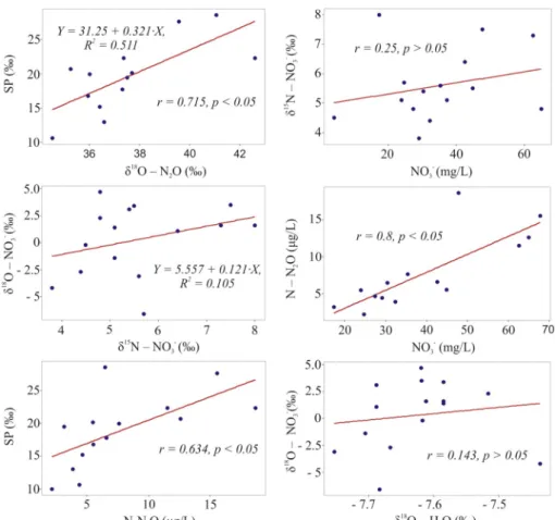
Pearson correlation analysis (Fig. 3) revealed high positive corre-lation between SP and δ18OeN
2O (r = 0.7, p < 0.05), while linear regression indicated positive dependency with the slope of 0.3 between these variables, which according toOstrom et al. (2007)(and references therein) should suggest the occurrence of incomplete denitrification in the aquifer (while the slopes close to 2.2 indicate the occurrence of N2O reduction in the absence of N2O production). However, the absence of correlation between δ15NeNO
3-and NO3−(r = 0.25, p > 0.05) and relationship between δ15NeNO
3- and δ18OeNO3 -(Y = 5.557 + 0.1212X, R2= 0.105) does not support the hypothesis about ongoing denitrification, because this process should lead to a strong negative correlation between δ15NeNO
3-and NO3−, and a slope of regression between δ15NeNO
3-and δ18OeNO3-ranging from 0.5 to 0.8 (Aelion et al., 2009;Minet et al., 2017). Pearson analysis also in-dicated strong positive correlation between the concentrations of NO3− and N2O (r = 0.8, p < 0.5) and between SP and N2O (r = 0.6, p < 0.05), which also does not support the occurrence of denitrifica-tion (Ostrom et al., 2007;Jurado et al., 2017), but rather indicate on-going nitrification. Moreover, groundwater chemistry data from the unconfined part of the aquifer demonstrated that aerobic conditions prevail across the area of study (see section3.1.1), which also supports the idea regarding occurrence of nitrification, and inhibition of deni-trification. According to Wankel et al. (2006) andMcMahon and Böhlke (2006), the occurrence of nitrification can be evidenced by the ex-istence of correlation between δ18OeNO
3-and δ18OeH2O, while the absence of correlation, on the contrary, suggests ongoing denitrifica-tion. Nevertheless, as shown inFig. 7, there was no correlation between δ18OeNO
3-and δ18OeH2O (r = 0.1, p > 0.05). Moreover, the average theoretical δ18OeNO
3-nitrification values defined from the following equation (Aelion et al., 2009):
= +
O NO 2/3( O H O) 1/3( O O )
18
3 18 2 18 2 (3)
for the three unconfined zones of the studied aquifer (2.8 for the southern and central zones, and 2.7 for the north-eastern zone) were different from the obtained results of δ18OeNO
3-analyses (2.5 for the southern zone, 1 for the central zone and −2.4 for the north-eastern zone). However, it should be emphasized that the above equation is just a rough estimate, since isotope exchange of intermediates with water messes up the O-isotope signature (Casciotti et al., 2010).
Such mixed evidence regarding the ongoing N2O production/con-sumption processes, obtained from the application of statistical analysis to the data describing unconfined part of the aquifer, suggests that the occurrence and intensity of these processes vary throughout the aquifer across the zones with different environmental conditions.
The values of δ34SeSO
42-versus δ18OeSO42-isotopic signals were examined, since SO42− isotope measurements are a unique tool al-lowing to reveal the connection between denitrification and sulphide oxidation during autotrophic denitrification (Mayer, 2005). Fig. 4 shows the overlap between mineralization of organic matter and oxi-dation of sulphides processes in all three zones located in the un-confined part of the aquifer. However, exceptions from this trend were detected for two points in Overhaem (12 and 13), which fell into the range typical for anthropogenic sources, and one point in Bovenistier (26), which showed the values typical for sulphide oxidation. Samples from the northern zone showed SO42− isotope values reflecting sul-phide oxidation (points 7 and 9). So, the dominant process of SO42− and, consequently, N transformation in three unconfined zones cannot be clearly identified.
component matrices resulting from the SOM application to the dataset (Fig. 5). Visual inspection reveals clear positive correlation between concentrations of Fe, Mn and CH4, which are negatively correlated with DO, thus indicating variations in oxido-reduction conditions across the aquifer. Results also show similar distribution patterns for N2O and NO3−, suggesting nitrification as the production mechanism of N2O in groundwater (Hiscock et al., 2003; Koba et al., 2009; Minamikawa et al., 2011). However, there is no clear relationship between N2O and DO, which does not allow claiming that nitrification is the only pro-duction pathway for N2O. A positive correlation is also observed be-tween SP and δ18OeN
2O, which suggests the occurrence of deni-trification (as N2O reduction proceeds), which leads to the
simultaneous increase of both parameters (Well et al., 2005,2012). This evidence suggests that N2O production throughout the chalk aquifer could not be attributed unequivocally to one pathway, as none of them seems to be omnipresent and clearly dominant across the whole area under consideration. Therefore, it appears that intensity of N2O production/consumption processes might vary spatially both in lateral and vertical dimensions (i.e. the simultaneous occurrence of nitrifica-tion in the shallower part of the aquifer and denitrificanitrifica-tion in its deeper part).
In order to obtain better understanding into the spatial variability of subsurface processes, the clustering of the dataset was conducted by means of SOM, and the isotope signatures of samples belonging to Fig. 3. The results of Pearson correlation and linear regression analyses for the subset. of data representing the unconfined part of the aquifer.
Fig. 4. δ34S versus δ18O values of SO 42− for groundwater samples. The shape of the points shows affiliation to different zones presented in Fig. 1. Colors indicate different concentrations of SO42−in groundwater samples. The isotopic compositions for the SO42− sources are derived from Krouse and Mayer (2000), Mayer (2005) and Knöller et al. (2005). (For interpretation of the references to colour in this figure legend, the reader is referred to the Web version of this article.)
various clusters were analyzed using isotopomer maps in order to consider the probable occurrence of denitrification and nitrification.
Fig. 6 shows four different groups obtained by application of k-means clustering on SOM. The dark blue (Group 1), green (Group 2) and blue (Group 3) groups include all of the groundwater samples collected from the unconfined part of the aquifer, while yellow group (Group 4) covers all of the studied points from the northern confined zone.
Group 1 includes locations in the unconfined zone which are char-acterized with the lowest SP (mean 11.2‰ ± 1.6‰), the lowest con-centration of dissolved N2O (mean 3.5‰ ± 1.2‰), high DO level (mean 8.2 mg/L ± 1.9 mg/L) and low NO3− (mean 28.7 mg/ L ± 3.8 mg/L). Group 2 corresponds to the highest SP (mean 26.1‰ ± 3.4‰), the highest concentration of N2O (mean 13.6‰ ± 6.3‰), the lowest amount of DO (mean 5.7 mg/ L ± 2.4 mg/L) and the highest concentration of NO3−(mean 48.7 mg/ L ± 18.7 mg/L). Group 3 demonstrates intermediate values of these parameters (seeTable 1). Finally, Group 4 shows characteristic values for groundwater from the confined part of the aquifer, namely lowest concentrations of NO3−and DO (see section3.1.1andTable 3).
The majority of SP values are lower than typical SP for hydro-xylamine (NH2OH) oxidation (nitrification) reported in previous stu-dies. These data could support the hypothesis about the occurrence of both denitrification and nitrification processes with the following mixing of deep denitrified and shallow nitrified groundwater (which leads to the decrease in SP values produced by nitrification). To test this hypothesis, two isotopomer maps for the area of study (Figs. 7 and 8) were developed.
From the Δδ15N
NO3− - N2O (‰) versus SP (‰) isotopomer map (Fig. 7), it can be concluded that the majority of data points re-presenting the isotopic signatures of respective samples in the southern, central and north-eastern zones fall into the mixing zone between ni-trification and denini-trification processes. Groundwater samples from Group 1 (points 17, 23 and 18) seem to be affected the most by deni-trification in comparison to other samples, which is illustrated by their closer location to the denitrification box. However, in this group the denitrification in the deeper part of the aquifer was not complete, since Group 1 was characterized with the lowest SP, and the N2O reduction to N2produces SP values close to the ones caused by nitrification (Well et al., 2012). This hypothesis is also supported by the fact that the corresponding groundwater samples show high DO concentration (see Table 3), which would not be possible if mixing with anoxic waters (< 4 mg/L) occurred.
The isotopic signatures of Group 2 (sampling points 30, 31 and 4) indicate mixing between nitrified groundwater and deep groundwater where complete denitrification occurred. The intensive denitrification processes are evidenced by the fact that all points fall outside the mixing zone (Fig. 7) and are shifted in the direction corresponding to typical N2O reduction. In addition, the lowest DO concentration was observed in this group.
In Group 3 (seeFig. 7), all samples are slightly shifted to the right of the mixing zone, suggesting mixing between nitrified and reduced groundwater. However, compared to Group 2, N2O reduction processes are probably less pronounced because of the high DO concentrations observed for groundwater samples from Group 3.
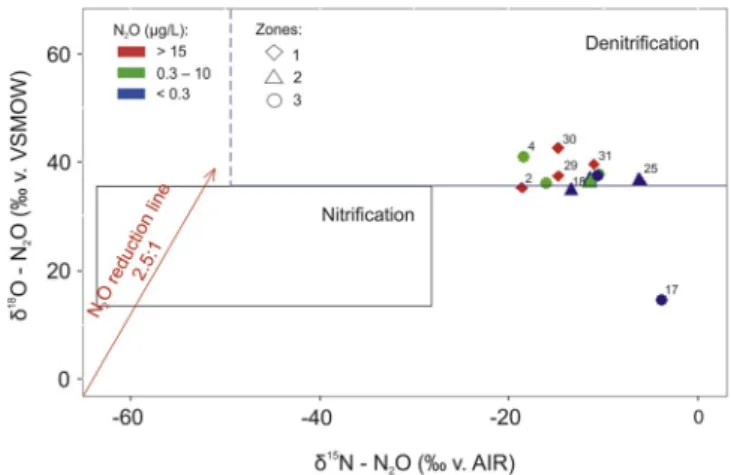
The second, δ15N e N
2O (‰ v. AIR) versus δ18O e N2O (‰ v. Fig. 5. The component matrices derived from the application of SOM procedure.
VSMOW) (Fig. 8), isotope map provides further evidence supporting the hypothesis that groundwater from the unconfined part of the aquifer is
majority of the samples fall close to the δ18O e N
2O value of +35‰, reported to be the boundary value between nitrification and deni-trification processes (Koba et al., 2009;Li et al., 2014).
Finally, in the northern zone, considering the low concentrations of DO and DOC as well as the data obtained from SO42−isotope analysis (Fig. 3), the occurrence of N2O could possibly be attributed to auto-trophic (points 9 and 7) or heteroauto-trophic (points 8, 14, 19 and 20) denitrification.
4.2.2. CH4production/consumption processes
The chalk aquifer was characterized with high level of CH4 accu-mulation despite the fact that there were detected high concentrations of DO, NO3−and SO42−in the unconfined part of the aquifer, and the high concentration of SO42−in the confined part of the aquifer (except point 14;Fig. S8of the supporting information), which prohibits CH4 production.
In the northern confined zone, characterized with low concentration of DO and negligible content of NO3−, the concentration of CH4was fifteen times higher in comparison to three other zones. At the same time, the concentration of SO42−, which varied from 15 mg/L to 90 mg/ L within the confined area, might have prohibited CH4production that usually occurs under lower SO42− concentrations (< 19 mg/L) (Whiticar, 1999;Molofsky et al., 2016).Whiticar (1999)claimed that methanogenesis using non-competitive substances (e.g. methylated amines or dimethyl sulphide) might occur in the media where SO42− exists; however, their relative importance in CH4 production is cur-rently uncertain. Therefore, the high values are more likely to be ex-plained by its thermogenic origin or presence of anaerobic microsites with favorable conditions within the aquifer.
The concentration of CH4 in the groundwater samples from southern, central and north-eastern zones could be explained by oc-currence of methanogenesis in the deeper part of the aquifer with the following mixing of deep CH4-enriched and shallow oxic water, which happened during the pumping activities. Moreover, the origin of CH4in the deeper part of the aquifer might be related to its upward migration via geological faults and fracture networks from the Houiller formations enriched in coal. This last assumption could be supported by previous investigations conducted by the Hydrogeology and Environmental Geology group of the University of Liege in 2015 which showed high accumulation of radon (28945 Bq/m3) in the deepest part of the aquifer at Bovenistier which might be the evidence of its origin from the un-derlying layers. Consequently, this observation suggests the possibility Fig. 6. Clustering of the groundwater samples using SOM algorithm. Group 1 –
dark blue, group 2 – green, group 3 – blue and group 4 – yellow. The numbers of sampled locations are presented within each of the group. (For interpretation of the references to colour in this figure legend, the reader is referred to the Web version of this article.)
Table 3
Mean hydrogeochemical parameters of the groundwater samples clusters pro-duced by k-means clustering on SOM.
Group N2O (μg N/L) SP (‰) DO (mg/L) NO3−(mg/L)
Group 1 3.4 ± 1.2 11.2 ± 1.6 8.2 ± 1.9 28.7 ± 3.8 Group 2 13.6 ± 6.3 26.1 ± 3.4 5.7 ± 2.4 48.7 ± 18.7 Group 3 6.7 ± 3.4 19.1 ± 6.7 7.2 ± 2.6 39.6 ± 16.2 Group 4 0.1 ± 0.1 not available 1.5 ± 2.1 0.2 ± 0.4
Fig. 7. Δδ15N
NO3−- N2Oversus SP (‰) isotopomer map. The shape of the points shows affiliation to different zones presented inFig. 1. Colors indicate different concentrations of NO3− in groundwater samples. (For interpretation of the references to colour in this figure legend, the reader is referred to the Web version of this article.)
Fig. 8. δ15N e N
2O (‰ v. AIR) versus δ18O e N2O (‰ v. VSMOW) isotopomer map. The shape of the points shows affiliation to different zones presented in Fig. 1. Colors indicate different concentrations of NO3−in groundwater sam-ples. (For interpretation of the references to colour in this figure legend, the reader is referred to the Web version of this article.)
considered impermeable.
In general, additional investigations are required in order to obtain better insight into the CH4production pathways. It will be useful to obtain data about the isotopic composition of CH4, δ13C-DIC and mi-crobiological community, which have been used in many studies for the identification of CH4 origin (Teh et al., 2005; Molofsky et al., 2013; McPhillips et al., 2014;Currell et al., 2017;Iverach et al., 2017).
4.2.3. CO2production/consumption processes
Groundwater in the chalk aquifer demonstrated a tendency towards accumulation of CO2. It is possible to suggest four pathways of the CO2 production in the subsurface, namely – rhizomicrobial and root re-spiration, microbial decomposition of soil organic matter, denitrifica-tion and, possibly, methane generadenitrifica-tion (Kuzyakov and Larionova, 2005).
First two processes lead to the production of CO2in the soil and its leaching into the groundwater during the rainy periods. The occurrence of microbial decomposition was evidenced by the data obtained from SO42− isotope analysis and parameters of water chemistry. In parti-cular, the observed SO42−isotope signals indicated the occurrence of mineralization processes in the subsurface, which under aerobic con-ditions produce SO42− and DOC (Mayer et al., 1995; Kellman and Hillaire-Marcel, 2003). However, according to the experimental data, the studied aquifer was characterized with low concentration of DOC in groundwater, which could be the consequence of its further oxidation to CO2in the unsaturated or saturated zones (MacQuarrie et al., 2001). The assumption regarding occurrence of DOC decomposition was also supported by the obtained strong negative correlation between the concentration of DOC and δ13C-DOC.
Since it was revealed that the aquifer was characterized with sui-table conditions for the occurrence of denitrification and methano-genesis processes in its deeper anoxic part, their contribution to the CO2 production could also be considered.
However, as our study was conducted in the chalk aquifer, the amount of dissolved CO2in the groundwater is strongly influenced by the calcium carbonate equilibrium. CO2, produced within or leaked to the aquifer, reacts with H2O to form H2CO3, a weak acid, which sti-mulates the dissolution of carbonate rocks. That is why, the initially produced concentration of CO2 will be altered by equilibration pro-cesses. In particular, saturation indexes (Text S1 of the supporting in-formation) varied from - 0.18 to 0.22 (mean 0.05 ± 0.08) for calcite and from −1.25 to −0.21 (mean −0.71 ± 0.23) for dolomite, in-dicating that groundwater was in equilibrium with respect to the first mineral and undersaturated with respect to the second one (Table S1of the supporting information) (Moore and Wade, 2013). This situation is attributed to the lower solubility of dolomite in comparison to calcite (Moore and Wade, 2013).
So, it appears that the latter two pathways of CO2production gov-erned the concentration of CO2in the northern confined zone, while in southern, central and north-eastern unconfined zones the presence of CO2was determined by the simultaneous occurrence of all processes discussed in this section.
4.3. Biogeochemistry of N2O, CH4and CO2. Vertical dimension 4.3.1. N2O production/consumption processes
According to the obtained hydrogeochemical and isotope data, ni-trification and denini-trification could be observed at different depths along the vertical profile of the studied aquifer. Also, these data provide evidence that mixing processes between the deep and shallow groundwater and slow infiltration of pollutants from the surface to the deeper parts of the aquifer affected the distribution of GHGs within the subsurface.
The high concentrations of DO, NO3− as well as δ15N and δ18O isotopic signatures of NO3− at two shallowest piezometers at Bovenistier 28 and 27 (Table 2) provided the evidence of N2O
production by nitrification processes. At the same time, the SP values of N2O at this site were considerably lower (19.2‰ and 20‰, respec-tively) than SP typically reported for nitrification. The analysis of SO42−isotopes showed that this location was the only one where ob-tained values of isotopic composition of the deepest groundwater (26) clearly fell into the range typical for sulphide oxidation (Fig. 3), which might be associated with autotrophic denitrification (Jurado et al., 2018b). Such evidence suggested that the isotopic signature of N2O of groundwater samples collected from the shallower part of the aquifer (28 and 27) was affected by both nitrification and denitrification pro-cesses (see section3.1.2.).
The anaerobic conditions and distribution of15N and18O isotopes of NO3−in the groundwater along vertical profile at Overhaem (10, 11 and 12) (Table 2) suggested the occurrence of denitrification. Since the SO42−isotopes did not indicate the occurrence of sulphide oxidation (Fig. 3), the occurrence of heterotrophic denitrification could be a production mechanism of N2O in this location.
The high level of DO, relatively high concentrations of NO3− (Table 2), results of NO3−and SO42−isotopes analyses (Figs. 2and3, respectively) at the SGB location (21, 22 and 25) indicated the occur-rence of nitrification processes. The SP value of N2O at the shallowest 21 piezometer was equal to almost 32‰, which also supported the idea about ongoing nitrification (Toyoda et al., 2017). However, the SP values of the groundwater samples collected from the deeper SGB 3 and SGB 1 piezometers were 14.1‰ and 15.2‰, respectively. Such data indicated that the production of N2O might be the result of the si-multaneous occurrence of both nitrification and denitrification or ni-trifier-denitrification processes in the groundwater system at SGB site.
4.3.2. CH4production/consumption processes
The concentration of CH4 (between 0.09 μg/L and 0.6 μg/L) was higher than equilibrium with the atmosphere concentration in all lo-cations across the vertical profile of the aquifer. However, no common trend in the distribution of CH4with depth for Bovenistier, Overhaem and SGB sampling locations was revealed.
The only site which showed the suitable conditions for the in situ biological production of methane was the deepest sampling point at Bovenistier (Table 2). As for the Overhaem and SGB, the high con-centrations of NO3−, SO4−and DO (only in case of SGB) along the whole depth interval excluded the possibility of methanogenesis. Therefore, detected co-existence of CH4with considerable concentra-tions of NO3−, SO42−and DO might be the evidence of its thermogenic origin and vertical migration through the system of fractures, surface contamination or methanogenesis that occur in anoxic microsites within the aquifer.
4.3.3. CO2production/consumption processes
The amount of CO2varied noticeably within the vertical profile of the aquifer from the lowest concentrations in deep groundwater to the highest concentrations in the shallow groundwater. Such distribution might be explained by stronger effects of rainwater on the composition of shallow groundwater and the decrease in the microbial activity with depth. In particular, it is likely that rain water washes out the CO2 produced in the soil due to the decomposition of DOC (see section 4.2.3.) and root respiration (Tan, 2010).
5. Conclusions
In this study the distribution of GHGs within the chalk aquifer under agricultural area was explored both across lateral and vertical dimen-sions. Lateral studies focused on the variability of GHGs concentrations taking into account the differences in hydrogeology, hydro-geochemistry and urbanization level across the explored region. Vertical dimension investigations attempted to elucidate the impact of heterogeneity of aquifer conditions along the depth profile on GHG concentrations.
Lateral explorations showed that among the three major GHGs it was the amount of N2O, which exhibited the greatest cross-zonal variability between identified zones with contrasting environmental settings. The highest concentration of N2O was detected in the un-confined aerobic part of the aquifer under most urbanized area where the concentration of NO3− was the highest, while the lowest N2O content was measured in the confined anaerobic zone with the very low or almost absent NO3− and/or NH4+ concentrations in the ground-water. In the zone of groundwater discharge to the Geer River, the average concentration of N2O was of the same magnitude as in the central zone, despite the fact that the NO3−content there was the lowest within the unconfined part of the aquifer. Also, in this zone the content of N2O varied significantly between different locations, as well as the level of DO, implying that the availability of N2O was governed by complex spatially heterogeneous pattern of different biogeochemical processes.
CH4 revealed the high tendency towards the accumulation in groundwater. Its concentration was substantially higher in the northern confined zone in comparison to three other zones. However, even in the unconfined southern, central and north-eastern zones despite the oxic conditions and presence of electron acceptors with higher energy yield the concentration of CH4 was, in average, approximately 13 times higher than its equilibrium atmospheric concentration.
Though the concentration of CO2 was high in comparison to its equilibrium concentration in the ambient air, it fluctuated less in comparison to N2O and CH4concentrations. CO2detected in the sub-surface derived from root respiration or decomposition of organic matter. However, the relative uniformity of its spatial distribution is mostly attributed to the fact that in general the amount of CO2 dis-solved in the groundwater was controlled by the process of dissolution of carbonate minerals which constitute aquifer geology.
The spatial differences in hydrogeochemical settings considerably influenced the dynamics of transformation of N and C loading in the subsurface, thus making tangible impact on the magnitude of the re-sulting indirect GHGs fluxes occurring on the groundwater-surface water interface. It was particularly noticeable in the case of highly volatile N2O production/consumption processes. The production of detected N2O could be attributed to a combination of nitrification and denitrification processes, likely occurring at different depths. However, the observed isotopic signals of N2O demonstrated that the intensity of these processes as well as their relative contribution to the concentra-tion of N2O in the groundwater varied across different sampling loca-tions.
Vertical dimension studies showed that different locations were characterized with different distribution pattern of major ions, GHGs and isotopes along the depth. However, in each of the cases they re-gistered the shift in concentration of CO2(decreasing with depth in all cases considered) and significant changes in both isotope signatures and concentration level of N2O across the depth profile. The latter ob-servation indicated that production/consumption dynamics of N2O was highly dependent on the hydrogeochemistry of the ambient subsurface environment. It was revealed that the variability of chemical compo-sition of groundwater in different locations was controlled by different biogeochemical processes changing in intensity with depth.
The observed heterogeneity of biogeochemical processes leading to GHGs production/consumption in the subsurface across the aquifer show that the magnitude of occurring GHGs fluxes (especially in the case of N2O in this study) could vary significantly due to the change in the amount of N and C inputs and distribution of their sources across different hydrogeochemical zones and in relation to groundwater flow pattern. Therefore, our study provides evidence to the assumption re-garding existence of uncertainty of indirect GHGs fluxes related to upscaling of the point-derived estimations to the catchment level. In order to reduce this uncertainty, it is advised before the estimation of GHGs fluxes at the groundwater – river interface (and possible
devel-insights obtained from larger-scale investigations in order to identify the representative spatial zones which shape the dynamics of GHGs emissions. As demonstrated by the results of combined application of SOM-derived clustering and interpretation of isotopomer maps, com-bination of insights from hydrogeochemical and isotope studies is es-sential in this regard, as it helps to get more profound insight into the process dynamics within the underground environment where the mi-crobiological structure and aquifer matrix might be additional factors that affect the transformation of N and C compounds. Moreover, due to the high heterogeneity of N and C sources and subsurface processes, it is particularly important to pay attention to the biogeochemical processes and modeling of GHGs transport in the hyporheic zone, since this zone is the buffer controlling the highly volatile dynamics of GHGs fluxes at the groundwater-river interface. In addition, further research efforts within the case study area are necessary in order to better understand the influence of fluctuating piezometric levels on the dynamics of hy-drogeochemical processes and GHGs production/consumption. Declarations of interest
None.
Acknowledgments
This project has received funding from the European Union's Horizon 2020 research and innovation programme under the Marie Skłodowska-Curie grant agreement No 675120. A.V.B. is a senior re-search associate the Fonds National de la Recherche Scientifique. Tanguy Robert is a F.R.S.eFNRS postdoctoral researcher.
Appendix A. Supplementary data
Supplementary data to this article can be found online athttps:// doi.org/10.1016/j.apgeochem.2019.04.009.
References
Aelion, C.M., Höhener, P., Hunkeler, D., Aravena, R. (Eds.), 2009. Environmental Isotopes in Biodegradation and Bioremediation. CRC Press.
Anderson, T.R., Groffman, P.M., Kaushal, S.S., Walter, M.T., 2014. Shallow groundwater denitrification in riparian zones of a headwater agricultural landscape. J. Environ. Qual. 43 (2), 732–744.
Battin, T.J., Luyssaert, S., Kaplan, L.A., Aufdenkampe, A.K., Richter, A., Tranvik, L.J., 2009. The boundless carbon cycle. Nat. Geosci. 2 (9), 598.
Beaulieu, J.J., Tank, J.L., Hamilton, S.K., Wollheim, W.M., Hall, R.O., Mulholland, P.J., et al., 2011. Nitrous oxide emission from denitrification in stream and river networks. Proc. Natl. Acad. Sci. Unit. States Am. 108 (1), 214–219.
Bell, R.A., Darling, W.G., Ward, R.S., Basava-Reddi, L., Halwa, L., Manamsa, K., Dochartaigh, B.Ó., 2017. A baseline survey of dissolved methane in aquifers of Great Britain. Sci. Total Environ. 601, 1803–1813.
Borges, A.V., Darchambeau, F., Teodoru, C.R., Marwick, T.R., Tamooh, F., Geeraert, N., et al., 2015. Globally significant greenhouse-gas emissions from African inland wa-ters. Nat. Geosci. 8 (8), 637.
Boulvain, F., Pingot, J.L., 2008. Une introduction à la géologie de la Wallonie.
Brouyère, S., Dassargues, A., Hallet, V., 2004. Migration of contaminants through the unsaturated zone overlying the Hesbaye chalky aquifer in Belgium: a field in-vestigation. J. Contam. Hydrol. 72 (1–4), 135–164.
Bunnell-Young, D., Rosen, T., Fisher, T.R., Moorshead, T., Koslow, D., 2017. Dynamics of nitrate and methane in shallow groundwater following land use conversion from agricultural grain production to conservation easement. Agric. Ecosyst. Environ. 248, 200–214.
Butterbach-Bahl, K., Well, R., 2010. Indirect emissions of nitrous oxide from nitrogen deposition and leaching of agricultural nitrogen. In: Nitrous Oxide and Climate Change. Routledge, pp. 166–193.
Casciotti, K.L., Sigman, D.M., Ward, B.B., 2003. Linking diversity and stable isotope fractionation in ammonia-oxidizing bacteria. Geomicrobiol. J. 20 (4), 335–353.
Casciotti, K.L., McIlvin, M., Buchwald, C., 2010. Oxygen isotopic exchange and fractio-nation during bacterial ammonia oxidation. Limnol. Oceanogr. 55 (2), 753–762.
Choi, B.Y., Yun, S.T., Mayer, B., Chae, G.T., Kim, K.H., Kim, K., Koh, Y.K., 2010. Identification of groundwater recharge sources and processes in a heterogeneous alluvial aquifer: results from multi-level monitoring of hydrochemistry and en-vironmental isotopes in a riverside agricultural area in Korea. Hydrol. Process. 24 (3), 317–330.