Inverse modelling of desorption tests to establish the hydraulic conductivity of unsaturated sands

(1)

INVERSE MODELLING OF DESORPTION TESTS TO

ESTABLISH THE HYDRAULIC CONDUCTIVITY OF

UNSATURATED SANDS

Mémoire

Seyed Mohammad Javad Hosseini Siahdashti

Maîtrise en génie civil

Maître ès sciences (M.Sc.)

Québec, Canada

(2)

(3)

iii

Résumé

Conductivité hydraulique non saturée est un paramètre important pour caractériser le comportement des sols non saturés. Ce paramètre peut être utilisé pour modéliser l'écoulement de l'eau dans les sols. Le défaut de mesure ou d'estimation de ce paramètre avec une précision fiable peut causer des incidents catastrophiques.

La mesure de la conductivité hydraulique des sols non saturés peut être longue et coûteuse. Des méthodes directes et indirectes peuvent être utilisées pour établir ce paramètre. Dans cette étude, en vue de réduire le temps et le coût de la mesure de la conductivité hydraulique des sols non saturés nécessaires par les méthodes directes, la modélisation inverse a été utilisée comme une méthode indirecte pour estimer ce paramètre. Des essais de laboratoire ont été effectués pour trouver la courbe de rétention d'eau des différents échantillons de sol étudié. Les résultats expérimentaux obtenus ont été utilisés pour effectuer la modélisation inverse, et la conductivité hydraulique non saturée de chaque échantillon a été estimé.

(4)

(5)

v

Abstract

Unsaturated hydraulic conductivity is an important parameter to characterize unsaturated soils behaviour. This parameter can be used to model flow of water in soils. Failure in measuring or estimating this parameter with a reliable precision can cause catastrophic incidents.

Measuring unsaturated hydraulic conductivity can be expensive and time consuming. Direct and indirect methods can be used to determine this parameter. In this study, in order to decrease the time and the expense of measuring unsaturated hydraulic conductivity by direct methods, inverse modelling was used as an indirect method to estimate this parameter. Some laboratory tests were performed to find water retention curve of different samples of the studied soil. Obtained experimental results were used to perform inverse modelling, and unsaturated hydraulic conductivity of each sample was estimated.

(6)

(7)

vii

List of Tables

TABLE 1:SAMPLES’ GRAIN SIZE CHARACTERISTICS ... 53

TABLE 2:HYDRAULIC PROPERTIES OF THE POROUS PLATE ... 60

TABLE 3:INVERSE MODELLING INITIAL AND OPTIMIZED VALUES FOR VAN GENUCHTEN MODEL ... 73

TABLE 4:INVERSE MODELLING INITIAL AND OPTIMIZED VALUES FOR FREDLUND &XING MODEL ... 73

TABLE 5:INVERSE MODELLING FIXED VALUES FOR VAN GENUCHTEN MODEL ... 81

TABLE 6:INVERSE MODELLING INITIAL AND OPTIMIZED VALUES FOR VAN GENUCHTEN MODEL ... 82

TABLE 7:COMPARISON BETWEEN POROSITY AND SATURATED HYDRAULIC CONDUCTIVITY OF TESTED MATERIALS WITH FILLION (2008) VALUES ... 93

(10)

(11)

xi

List of Figures

FIGURE 1:DISTRIBUTION OF DIFFERENT PHASES IN SOIL ... 5

FIGURE 2:RISING WATER IN A CAPILLARY TUBE (INSPIRED FROM FREDLUND &RAHARDJO,1993) ... 7

FIGURE 3:WATER IN SOIL PORES AND TENSIONS BETWEEN WATER AND SOIL PARTICLES SURFACE FROM A SATURATED STATE TO A DRY STATE (INSPIRED FROM FAROUK ET AL.2004) ... 8

FIGURE 4:CONCEPTUAL SKETCH SHOWING THE RELATIONSHIP BETWEEN PORE SIZES, CAPILLARY RISE IN TUBE AND THE SWRC (ADAPTED FROM TULLER AND OR 2003) ... 9

FIGURE 5: A)TENSIOMETER,MODEL:2710ARL(SOILMOISTURE EQUIPMENT CORP.)... 11

FIGURE 6:SCHEMATIC VIEW OF THE NULL TYPE PRESSURE PLATE APPARATUS (FREDLUND &RAHARDJO, 1993) ... 12

FIGURE 7:SCHEMATIC OF CHILLED-MIRROR DEW-POINT DEVICE (TRIPATHY ET AL.2003) ... 13

FIGURE 8: PHOTOGRAPH OF A CHILLED MIRROR HYGROMETER (ASTM-D6836-02,2012) ... 13

FIGURE 9:CERAMIC SHIELDED THERMOCOUPLE PSYCHROMETER (COKCA,2000) ... 15

FIGURE 10:SCHEMATIC VIEW OF AN SMI TRANSISTOR PSYCHROMETER (CARDOSO ET AL.2007) ... 16

FIGURE 11:A CROSS SECTIONAL DIAGRAM OF THE THERMAL CONDUCTIVITY SENSOR (SATTLER & FREDLUND,1989) ... 19

FIGURE 12:TYPICAL SWRC, WETTING AND DRYING CURVES ... 22

FIGURE 13:TYPICAL SWRC FOR SANDY SOIL, SILTY SOIL AND CLAYEY SOIL ... 22

FIGURE 14:USE OF THE AXIS TRANSLATION TECHNIQUE TO AVOID METASTABLE STATES ... 24

FIGURE 15:PHOTOGRAPH OF A FUNNEL USED FOR HANGING COLUMN APPARATUS (ASTM-D6836–02, 2012) ... 26

FIGURE 16:SCHEMATIC VIEW OF A HANGING COLUMN APPARATUS (ASTM-D6836–02,2012) ... 27

FIGURE 17:5BAR PRESSURE PLATE EXTRACTOR, PICTURE FROM SOILMOISTURE EQUIPMENT CORP. (SOILMOISTURE.COM) ... 27

FIGURE 18:CROSS SECTIONAL VIEW OF THE SKETCH OF A TEMPE CELL (SOILMOISTURE EQUIPMENT CORP. 1995) ... 28

FIGURE 19:SOME COMMON SOIL WATER CONTENT MEASUREMENT METHODS AND THEIR CORRESPONDING MATRIC SUCTION RANGES (TULLER &OR,2003) ... 29

FIGURE 20:COMPARISON OF SWRC RESULTS BETWEEN BROOKS AND COREY AND DATA FOR PACHAPPA LOAM (ASSOULINE &TARTAKOVSKY,2001) ... 33

FIGURE 21:COMPARISON BETWEEN MEASURED DATA AND ARIA AND PARIS (1981) MODEL PREDICTED VALUES OF SWRC FOR TWO JERSEY SOILS (ARYA &PARIS,1981) ... 34

FIGURE 22:AFREDLUND &XING (1994) MODEL BEST-FIT CURVE TO THE EXPERIMENTAL DATA OF A SANDY MATERIAL ... 35

(12)

FIGURE 23:SCHEMATIC VIEW OF A CENTRIFUGE PERMEAMETER WITH RELEVANT VARIABLES (REPRINTED

FROM ZORNBERG &MCCARTNEY,2010) ... 39

FIGURE 24:EXPERIMENTAL SETUP FOR WENDROTH ET AL.(1993) ... 40

FIGURE 25:COMPARISON OF RELATIVE HYDRAULIC CONDUCTIVITY RESULTS BETWEEN BROOKS AND COREY AND EXPERIMENTAL DATA FOR PACHAPPA LOAM (ASSOULINE &TARTAKOVSKY,2001) ... 42

FIGURE 26:A BEST-FIT CURVE OF VAN GENUCHTEN MODEL TO THE EXPERIMENTAL DATA OF HYGIENE SANDSTONE – (VAN GENUCHTEN,1980) ... 43

FIGURE 27:FLOW CHART OF THE INVERSE METHOD ILLUSTRATING THE STEPS OF INVERSE MODELLING (REPRINTED FROM HOPMANS ET AL.2002) ... 47

FIGURE 28:EDS RESULTS FOR THREE PARTICLES OF THE TESTED SOIL ... 52

FIGURE 29:SOIL SAMPLES GRAIN SIZE DISTRIBUTION ... 53

FIGURE 30:HIGH-RESOLUTION PICTURES OF TESTED SOIL SAMPLES ... 55

FIGURE 31:ELECTRONIC PHOTO OF A 160 µ PARTICLE ... 57

FIGURE 32:SKETCH OF THE CELL USED IN THE SCOPE OF THIS STUDY ... 59

FIGURE 33:DIFFERENT PARTS OF THE DEVELOPED CELL IN THE SCOPE OF THIS STUDY ... 60

FIGURE 34:TENSIOMETER USED IN THE SCOPE OF THIS RESEARCH ... 61

FIGURE 35:APPARATUS THAT WAS USED TO SATURATE SOIL SPECIMEN AND THE POROUS PLATE ... 64

FIGURE 36:PRESSURE AND VOLUME CHANGE CONTROLLER ... 64

FIGURE 37:APPARATUS THAT WAS USED TO SATURATE THE SOIL SPECIMENS ... 67

FIGURE 38:SCHEMATIC VIEW OF THE SOIL SUCTION IN DIFFERENT ELEVATIONS OF THE SOIL PROFILE ... 69

FIGURE 39:CUMULATIVE OUTFLOW AND SOIL SUCTION CURVES OBTAINED BY LABORATORY RESULTS,[S-1] ... 69

FIGURE 42:MEASURED SUCTIONS AT THREE DIFFERENT LEVELS IN THE SOIL PROFILE,[S-1] ... 71

FIGURE 45:SOIL WATER RETENTION CURVE, EXPERIMENTAL RESULTS, VAN GENUCHTEN (1980) AND FREDLUND &XING (1994) MODELS FITTED TO MEASURED DATA,[S-1] ... 74

(13)

xiii

FIGURE 48:EFFECT OF GRAIN SIZE DISTRIBUTION AND COEFFICIENT OF UNIFORMITY ON SOIL WATER

RETENTION RESULTS OF THE SOIL SAMPLES ... 76

FIGURE 49:COMPARISON BETWEEN PREDICTED RELATIVE UNSATURATED HYDRAULIC CONDUCTIVITIES (FREDLUND EL AL. AND VAN GENUCHTEN MODELS),[S-1]... 78

FIGURE 50:COMPARISON BETWEEN PREDICTED RELATIVE UNSATURATED HYDRAULIC CONDUCTIVITIES (FREDLUND ET AL. AND VAN GENUCHTEN MODELS),[S-2] ... 78

FIGURE 51:COMPARISON BETWEEN PREDICTED RELATIVE UNSATURATED HYDRAULIC CONDUCTIVITIES (FREDLUND ET AL. AND VAN GEUNCHTEN MODELS),[S-3] ... 79

FIGURE 52:COMPARISON BETWEEN OBSERVED AND INVERSE MODELLING FITTED VALUES,[S-1]... 83

FIGURE 55:COMPARISON BETWEEN LABORATORY AND INVERSE MODELLING SWRC RESULTS ... 87

FIGURE 56:UNSATURATED HYDRAULIC CONDUCTIVITY OBTAINED BY INVERSE MODELLING,[S-1] ... 89

FIGURE 59:COMPARISON BETWEEN POROSITY AND SATURATED HYDRAULIC CONDUCTIVITY OF TESTED MATERIALS WITH FILLION (2008) OBTAINED VALUES ... 93

FIGURE 60:COMPARISON OF RELATIVE HYDRAULIC CONDUCTIVITIES OF TESTED SAMPLES ... 94

FIGURE 61:COMPARISON OF RELATIVE UNSATURATED HYDRAULIC CONDUCTIVITIES OBTAINED BY INVERSE SOLUTION,FREDLUND MODEL AND VAN GENUCHTEN MODEL ... 96

(14)

(15)

xv

List of Abbreviations

AEV AIR-ENTRY VALUE

BC BROOKS AND COREY

EDS ENERGY DISPERSIVE SPECTROSCOPY

IPM INSTANTANEOUS PROFILE METHOD

MSO MULTI-STEP OUTFLOW

OSO ONE-STEP OUTFLOW

SWCC SOIL WATER CHARACTERISTIC CURVE

SWRC SOIL WATER RETENTION CURVE

(16)

(17)

xvii

Acknowledgements

First and foremost I wish to thank my advisor Dr. Jean Côté, the Associate Chairholder of the NSERC-Hydro-Québec Industrial Research Chair in life cycle optimization for embankment dams. He has been supportive since I began my master studies.

I would like to thank Dr. Jean-Marie Konrad and Dr. Jean-Pascal Bilodeau, whose detailed remarks and comments improved the quality of this manuscript, and François Gilbert, Christian Juneau, Luc Boisvert, and Marc Lebeau for their help during my experiments. For financial support for my studies, I am grateful to Laval University, Hydro-Quebec, and other partners of the NSERC-Hydro-Québec Industrial Research Chair in life cycle optimization for embankment dams.

I want to thank my friends and fellow graduate students for being supportive through these recent years.

Finally, I am grateful to my dear parents, my brother and my lovely sister. They always supported me, and they were always there for me. Thank you.

(18)

(19)

1

1 Introduction

This research aims to find ways to decrease the required time and expense of measuring hydraulic properties of soils directly by laboratory tests. Numerical models have been developed to simulate water movement in porous media. These models can be used to estimate hydraulic conductivity of unsaturated soils by using water retention data. There are different methods to determine water retention data. For the purpose of this study, transient outflow method was used to determine water retention data in laboratory.

This research attempts to characterize the retention and hydraulic properties of sandy materials in an unsaturated state. Some transient flow tests have been performed to measure soils water retention values. These values were then used to simulate water movement and estimate unsaturated hydraulic conductivity by inverse modelling. This reduced the time and expenses of the tests. To achieve this goal, an experimental procedure had been developed to simulate seepage in transient flow to measure hydraulic conductivity.

Laboratory tests were performed under controlled conditions with well-defined initial and boundary conditions. The flow variables were measured in each test. The water flow was written with mathematical relations. A numerical model was used and inverse modelling was performed by minimizing the difference between observed laboratory results and estimated flow variables.

To understand hydraulic functions of unsaturated soils, it is necessary to understand different phases of unsaturated soils. Chapter 2 deals with definition of unsaturated soils and capillary mechanism. This chapter also describes soil water retention curve and its components (water content and soil suction) and different methods of measuring or estimating these values. There are different methods that have been used to model soil water retention curve in literatures such as Brooks & Corey (1964), Fredlund & Xing (1994) and van Genuchten (1980). These methods are also reviewed in this chapter.

In chapter 3 the theory of inverse methods is discussed. Richards’ equation is used to express water flow in unsaturated soils. Then the parameter optimization is reviewed.

(20)

2

Chapter 4 focuses on the performed experiments in the scope of this study and the specification of the materials that was tested to find its unsaturated hydraulic conductivity. In this chapter multi-step outflow experiment is discussed and different steps of experimental protocol is reviewed.

In chapter 5 experimental results of the performed multi-step outflow method experiments is summarized. These results include soil pressures in three different elevations of soil samples and amount of extracted water for each pressure step. By using our laboratory results, soil water retention curve is determined for each material. Soil water retention curve of each sample is discussed based on its grain size distribution and the coefficient of uniformity.

Chapter 6 reviews unsaturated hydraulic conductivity results for each sample. Different methods are used to determine unsaturated hydraulic conductivity of each material. These methods includes van Genuchten (1980) and Fredlund et al. (1994) models. These results are then compared with inverse modelling results.

(21)

3

2 Unsaturated Soils

2.1 Unsaturated Soil Definition

Most geotechnical engineering projects that include water flow in soil are related to the unsaturated soils. For example, during the construction of an earth fill dam, the soil is normally compacted with a degree of saturation about 80%. After construction and during the filling period, the dam will face different unsaturated zones. When the dam’s reservoir is fully filled with water, some regions in dam structure remain unsaturated.

As another application, road pavements are constructed with compacted unsaturated soils with degree of saturation between 75-90 %. Pavement’s stiffness and strength are significantly influenced by soil suction due to the presence of water between soil particles. About a century ago, Buckingham (1907) was one of the pioneers who worked on multiphase flow. This was the basis of studies on unsaturated soils. An unsaturated soil is a system that contains three different phases, namely as soil particles, water, and gas. Each phase has its own specified volume and mass fraction. Fredlund & Rahardjo (1993) proposed the air-water interface as the fourth phase of unsaturated soils. This phase was called contractile skin.

Unsaturated soils behave differently in comparison with the saturated soils. These differences are mainly related to the mechanical and hydraulic properties. Therefore, knowing these differences and their effects are essential in designing a geotechnical structure.

Generally, the geotechnical problems of unsaturated soils are related to volume changes, shear strength and hydraulic flow in the soil.

Shear strength is one of the most important parameter in unsaturated soils that has to be considered during soil analysis. Many reported failures in dams, embankments and slopes during past decades were related to miscalculation of the shear strength in unsaturated soils.

(22)

4

Classical soil mechanics cannot be used to determine the mechanical properties of unsaturated soils, and they are proper to determine the mechanical properties of saturated soils. Tarantino (2007), Sun et al. (2003) and Alonso et al. (1990) proposed several failure criteria that can be used to predict shear strength of unsaturated soils.

Volume change can cause settlements leading to damages in structures like embankments. Fredlund et al. (2000) conducted some experiments to estimate volume change functions for unsaturated soils. Fredlund et al. (2000) provided a series of postulates based on saturated volume change and using soil water characteristic curve information.

Soil is composed of particles that are in contact with each another. These particles have different shapes and sizes. These differences lead to different pore sizes in soil. These pores act like tubes with different radii. Due to capillary forces in a narrow tube, water tends to move upward. Capillary forces have inverse relation with the tube diameter.

2.1.1 Water Content

The ratio between different phases of soil gives different properties to the system. Therefore, having a good knowledge on these ratios will be useful to predict the soil properties. “Degree of saturation” is one of the definitions that is normally used while studying unsaturated soils. This parameter is shown by “𝑆𝑟” and defines the percentage of voids filled with water.

𝑆𝑟 (%) = 𝑉_𝑉𝑤

𝑣 × 100

Equation 1

where 𝑉𝑤 is the water volume and 𝑉𝑣 is the total void volume (Figure 1). The lower and upper limits for 𝑆𝑟 are 0% and 100% for utterly dried and fully saturated soils, respectively. To quantify the amount of water in porous materials such as soil, “water content” parameter, 𝜃 can be expressed as:

(23)

5 Figure 1: Distribution of different phases in soil

𝜃(%) = _𝑉𝑉𝑤

𝑡𝑜𝑡𝑎𝑙 × 100

Equation 2

where 𝑉𝑡𝑜𝑡𝑎𝑙 is the total volume and is equal to the sum of volumes of soil, water and air. Water content is also known as moisture content and varies between 0% to 100%.

There are direct and indirect methods to measure or estimate soil water content. Direct methods are based on extracting water from the soil sample. Leaching and evaporation, for example, are the methods that can be used to directly measure the water content of the soil. In direct methods, water removed from the sample is directly measured by weight. Besides the direct methods, some indirect methods can also be used to find soil water content. In these methods, another material like an absorber is normally used. By placing these materials in soil and measuring its properties, water content can be measured.

(24)

6

2.1.2 Soil Suction

Soil suction (total suction), which is defined in term of the energy state of the soil water system, has two different components; matric component and osmotic component. Soil suction can be written as:

𝜓 = (𝑢𝑎− 𝑢𝑤) + 𝜋 _{Equation 3}

where 𝜓 is the soil suction, (𝑢𝑎− 𝑢𝑤) is the matric suction which is also known as capillary pressure, 𝜋 is the osmotic suction, 𝑢𝑎 and 𝑢𝑤 are the pore air and pore water pressure, respectively. All are measured in kPa.

As shown in Figure 2 (Inspired from Fredlund & Rahardjo, 1993), the level of the water in a tube connected to a water container rises because of the capillary phenomenon. This phenomenon happens because of surface tension in the contractile skin. These forces cause a curved surface at the top of the water level in the tube. The height of the water in the tube can be found by using capillary equation:

2𝜋𝑟𝑇𝑠 𝑐𝑜𝑠𝛼 = 𝜋𝑟2ℎ𝜌𝑤𝑔 _{Equation 4}

where 𝑟 is the radius of the capillary tube, 𝑇𝑠 is the surface tension of water, 𝛼 is the contact angle, 𝜌𝑤 is the density of water, 𝑔 is the gravitational acceleration and ℎ is the capillary height. Solving the Equation 4 for h gives the height of raised water in the capillary tube:

ℎ = 2𝑇𝑠 𝑐𝑜𝑠𝛼/𝑟𝜌𝑤𝑔 _{Equation 5}

Considering an equilibrium condition and applying the Pascal’s law between the points A and B, one can write:

𝑢𝑤 = −𝜌𝑤𝑔ℎ _{Equation 6}

where 𝑢𝑤 is the hydrostatic pressure at point A. At this point, the value of air pressure is set to zero. Therefore:

(25)

7 Figure 2: Rising water in a capillary tube

(Inspired from Fredlund & Rahardjo, 1993)

𝑻𝒔 𝑻𝒔 𝜶 𝒉 𝑨 A B (𝑢𝑎− 𝑢𝑤) = 𝜌𝑤𝑔ℎ = 2𝑇𝑠 𝑐𝑜𝑠𝛼/𝑟 _{Equation 7}

Based on the Equation 7, when radius of the tube decreases, matric suction (ua− uw) increases.

As it was mentioned earlier, soil is composed of particles of different shapes and sizes. Because of these differences, pores between these particles have irregular shapes and sizes. These pores can be simplified as tubes with different sizes. These tubes could either be fully or partially filled with water, or empty. As is seen in Figure 3-b when the soil is partially saturated an air- water interface is formed between soil’s particles. This interface has a curved meniscus. Capillary pressure is the pressure difference between ambient air and water phase in their interface (Karkare & Fort, 1993).

Capillary pressure is an inter-granular pressure between soil particles. In Figure 3 (Inspired from Farouk et al. 2004) water in soil pores and tensions between water and soil particles surface from a saturated state to a dry state is illustrated. In this figure, “a” shows two soil particles in a saturated state, while “b” and “c” illustrate these particles in an state between fully saturated and dried conditions. Tensions on soil particles due to the presence of water

(26)

8

between these particles are illustrated by the black vectors. In Figure 3, “d” shows a fully dried soil.

Figure 4 (adapted from Tuller & Or 2003) illustrates a conceptual sketch of relationship between pore sizes and capillary rise in tube. As it can be seen, in smaller pores capillary rises are greater. The dark blue color shows the rising water in each tube with a certain diameter due to capillary phenomenon. Soil water content at each elevation will be the accumulated volume of water in all tubes from z=0 to that certain elevation.

Due to the capillarity phenomenon, the degree of saturation above the water surface (capillary zone) is less than 100 percent. In capillary zone, pressure is negative and less than atmospheric pressure.

Figure 3: Water in soil pores and tensions between water and soil particles surface from a saturated state to a dry state (Inspired from Farouk et al. 2004)

a) Saturated b and c) Unsaturated d) Dry

a

b

(27)

9 Figure 4: Conceptual sketch showing the relationship between pore sizes,

capillary rise in tube and the SWRC (Adapted from Tuller and Or 2003)

As it was mentioned earlier, total suction has two components, osmotic suction and matric suction. Measuring matric suction in soil, particularly in high pressures is not easy. Since the osmotic suction does not have a great influence on water content of the soils, the total suction can be used as a representative for soil suction (Fredlund & Rahardjo, 1993). There are different instruments, that can be used to measure soil matric or total suction. These

(28)

10

instruments are designed to measure soil suction in field or laboratory. These methods can be divided into two major groups, Direct methods and Indirect methods.

2.1.2.1 Direct Methods for Measuring Soil Suction

There are different instruments and techniques, which were developed during the past decades to measure soil matric or total suction. Tensiometers and null type pressure plates are examples of equipment that are used to measure matric suction. To measure soil total suction directly, the chilled mirror dew-point apparatus and psychrometer can be used. 2.1.2.1.1 Tensiometer

Tensiometer is an instrument to measure soil matric suction directly. Richards & Gardner (1936) and Richards (1941) were among the firsts who designed and used the tensiometer. As it can be seen in Figure 5-a (Soilmoisture Corp.), this instrument consists of a porous cup (normally ceramic) which is connected to a vacuum gauge through a rigid body tube. To measure soil suction, tensiometer should be saturated. Tensiometer’s cup is inserted in the soil with a good contact to the soil particles. Water moves through the cup and after a while tensiometer equilibrate with water in the soil. These types of tensiometers are called vacuum gauge tensiometers. Presence of air in the water column will reduce accuracy of the tensiometer and increases measurement’s time (Smajstrla & Harrison, 1998). Some models of tensiometers include a transducer. These transducers are connected to data loggers and can continuously record pressure values. Due to the cavitation problem, tensiometers can be used for low pressure ranges, normally lower than 90 (kPa) (negative pressure). The other problem is related to the air diffusion through the ceramic cup. This phenomenon can reduce the accuracy and response of the tensiometers (Fredlund & Rahardjo, 1993). The Jet-fill tensiometer was designed to reduce the air bubbles’ negative effect on the tensiometer’s results. This tensiometer can remove the accumulated air bubbles. As is shown in Figure 5-b (Soilmoisture Corp.), at the top of the jet-fill tensiometer a water reservoir is placed. This reservoir can be used to jet water into the tube to remove air bubbles.

(29)

11 Figure 5: a) Tensiometer, Model: 2710ARL (Soilmoisture Equipment Corp.)

b) Jet fill tensiometer (Eijkelkamp Agrisearch Equipment)

a

b

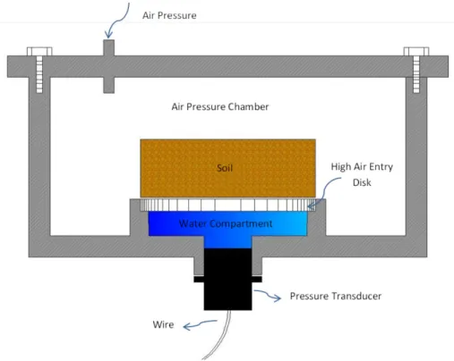
2.1.2.1.2 Null Type Pressure Plate

A null-type pressure plate is one of the instruments for measuring matric suction by direct methods. This instrument can be used to measure matric suction in laboratory for fine-grained unsaturated soil specimens by applying the axis translation technique and is suitable for pressures between 50-500 kPa. As seen in Figure 6 (Fredlund & Rahardjo, 1993), a high air-entry disk is inserted under the soil specimen. The soil specimen is placed in a chamber, which is air proof. Air pressure can be applied to get to desired soil suction. Soil suction is measured at each air pressure. The following apparatus was used for the axis translation technique.

2.1.2.1.3 Chilled Mirror Dew Point

There is a relation between the soil total suction and the water vapour pressure, so this property can be measured by devices that are used to measure relative humidity (Tripathy et al. 2003). Instruments and techniques used to measure the soil total suction include, chilled mirror dew-point device, paper method, psychrometer, and relative humidity.

(30)

12

Figure 6: Schematic view of the Null Type Pressure Plate apparatus (Fredlund & Rahardjo, 1993)

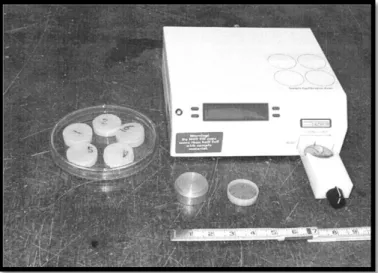
The Chilled mirror dew-point device can be used to measure soil total suction in laboratory. Dew-point is the temperature at which the water vapour in a volume of humid air at a constant pressure will condense into liquid water. In other words, at this point there is enough water vapour in the air to fully saturate it. A schematic view of a dew-point chilled mirror is shown in Figure 7 (Tripathy et al. 2003).

To use this device for measuring soil suction, a soil sample is prepared, placed into a container filling it half way and inserted into a sealed chamber. The soil equilibrates with the water vapour in the space around the soil sample. A mirror in the chamber is connected to a thermoelectric cooler. The temperature of the point that condensation happens is recorded by thermocouple attached to the mirror. To measure soil suction for different water contents, a series of specimens are prepared and for each the suction is measured. This method has an accuracy around ±0.1% (Tripathy et al. 2003).

(31)

13 Figure 8: Photograph of a Chilled Mirror Hygrometer (ASTM-D6836-02, 2012)

Figure 7: Schematic of chilled-mirror dew-point device (Tripathy et al. 2003)

Figure 8 (ASTM-D6836-02, 2012) is a photograph of a Chilled Mirror Hygrometer and the specimen to be tested.

As it was mentioned earlier, this method was developed for laboratory suction measurement; but recently some attempts were made to use a chilled mirror for field measurement (Richardson et al. 1999).

Fan

Soil Sample

Mirror and Photo -Detector Cell Temperature Sensor

(32)

14

2.1.2.1.4 Psychrometer

Psychrometer can measure soil total suction by measuring relative humidity in the air phase of soil pores or the region near the soil (Fredlund & Rahardjo, 1993). Psychrometers are generally used in laboratories. This instrument uses Kelvin’s Law to measure soil’s suction. This measuring technique has two main problems. The first problem relates to the small amount of relative humidity changes in the soil gas phase. The second problem originates from the fact that temperature differences in the sensor–sample system may cause large errors in water potential determination (Dane & Topp, 2002). There are different types of psychrometers. Most of them consist of two similar thermometers that are installed side by side. Psychrometers are of three major types:

a) Thermistor psychrometer b) Thermocouple psychrometer c) Transistor psychrometer

2.1.2.1.4.1 Thermocouple Psychrometer

Spanner (1951) was the first to introduce the thermocouple psychrometer. Spanner’s thermocouple psychrometer is limited by the required rigid temperature control (Kay & Low, 1970). Rawlins and Dalton (1967) did some modifications to improve Spanner’s psychrometer for in-situ measurements. Rawlins and Dalton used a Peltier cooling system to make a wet junction. The Peltier sensor is one of the two major sensor types that are used in thermocouple psychrometers.

The other type of sensor that is generally used in thermocouple psychrometers is called wet-loop sensor (Dane & Topp, 2002). Tensiometers have upper and lower boundaries for the pressure they can measure, and these limits are highly influenced by the sensor’s design and measurement protocol (Dane & Topp, 2002). Thermocouple psychrometers can measure the soil total suction at any point in the soil profile. The soil water potential gradient can be determined by its results (Enfield & Hsieh, 1971).

(33)

15 Figure 9 (Cokca, 2000) shows a schematic view of a ceramic shielded thermocouple psychrometer.

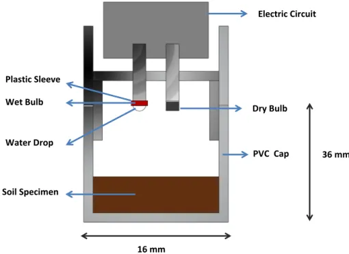
2.1.2.1.4.2 Transistor Psychrometers

This type of psychrometers also uses relative humidity to find soil total suction. In this type of psychrometer, the evaporating wet-bulb is wetted by placing a drop of water into a small ring in all the psychrometer’s probes. In Figure 10 (Cardoso et al. 2007) a schematic view of an SMI transistor psychrometer is given. These bulbs act as wet and dry thermometers. The difference in temperature between these two bulbs is used to measure relative humidity (Cardoso et al. 2007). The transistor psychrometer can be used to measure total suction in the range of 0.1 MPa to 10 MPa with good accuracy. Results obtained by Bulut et al. (2000) showed that at low suctions, this method is highly sensitive.

2.1.2.2 Indirect Methods to Measure Soil Suction

Beside direct methods of measuring soil total or matric suction, there are some indirect methods that can be used to find soil suction. These methods are influenced by different

(34)

16 Electric Circuit Dry Bulb PVC Cap Plastic Sleeve Soil Specimen Water Drop Wet Bulb 16 mm 36 mm

parameters that can affect their accuracy. Isothermal equilibrium between the sensor, and the vapour space in the closed system of measurement media has an effect on the indirect methods’ accuracy (Agus & Schanz, 2005).

2.1.2.2.1 Filter Paper Method

Gardner (1937) was the first who succeeded in using a filter paper to measure the soil matric and total suction. This method is based on measuring the amount of moisture transferred form an unsaturated soil sample to an initially dry filter to estimate soil suction (Likos & Lu, 1981).

The contact between the soil sample and filter paper plays an important role in the nature of the measured. If the filter paper is in contact with the soil sample, the water absorbed by the filter paper has the same concentration as the soil sample. In this case, the measured suction is matric suction. However, if there is no contact between the soil sample and the filter paper, the measured suction is equal to the soil’s total suction (Marinho & Oliveira, 2012).

Figure 10: Schematic view of an SMI transistor psychrometer (Cardoso et al. 2007)

(35)

17 This method uses Kelvin’s Law to find soil’s total suction by its relationship with the pore water vapour’s relative humidity (Agus & Schanz, 2005).

𝑆 = −𝑅𝑇

𝑀𝑊(1 𝜌� )_𝑊 𝑙𝑛 (𝑅𝐻)

Equation 8

where S is the total suction, R is the universal gas constant (8.32432 𝐽 𝑚𝑜𝑙−1_𝐾−1_{), T is the} absolute measured temperature (in Kelvin), 𝑀𝑊 is the molecular weight of water ( 18.016 𝑘𝑔 𝑘𝑚𝑜𝑙−1_{), 𝜌}

𝑊 is ythe unit weight of water (998 𝑘𝑔 ⁄ 𝑚3 at 20o 𝐶), as a function of temperature and 𝑅𝐻 is the measured relative humidity [𝑢𝑣⁄𝑢𝑣𝑜], where 𝑢𝑣 is the partial pressure of pore water vapour in the specimen and uvo is the saturation pressure of water vapour over a flat surface of water at the same temperature). At 20° C, Equation 8 becomes:

𝑆 = −135055 𝑙𝑛(𝑅𝐻) [𝑘𝑃𝑎] _{Equation 9}

The papers should be calibrated prior to starting each test. To calibrate the filter paper, the relationship between equilibrium water content of the filter paper and the relative humidity of vapour phase is determined (Likos & Lu, 1981). This calibration can be done by using a salt solution that has a known concentration. Pressure membranes (100 kPa to 1500 kPa) or the ceramic plate (10 kPa to 100 kPa) can also be used to calibrate filter paper (ASTM-5298-10, 2010).

Likos and Lu (2002) have done two series of tests to evaluate the accuracy of noncontact filter paper technique for total suction testing. Their results shown that the filter paper calibration curves can vary significantly from batch to batch. Based on their studies, they recommended independent calibration from batch to batch. They had also shown that by decreasing total suction, uncertainty in total suction measurement by using the noncontact filter increases dramatically.

2.1.2.2.2 Thermal Conductivity Sensors

Shaw and Baver (1939) introduced a technique to measure soil suction by using thermal properties of water. They used heat conductivity as an index of the changing moisture

(36)

18

condition in-situ. Thermal conductivity method is one of the best instruments of measuring soil matric suction. This method is based on thermal conductivity of air and water. Thermal conductivity of water is better than thermal conductivity of air. When percentage of air in soil decreases, total thermal conductivity will decrease. Thermal conductivity sensors use this difference to measure soil suction. The accuracy measurements of thermal conductivity sensors are influenced by their calibration (Fredlund & Wong, 1989; Leong et al. 2012; Wong et al. 1989). Calibration of thermal conductivity device is the first step in using it for measuring soil suction.

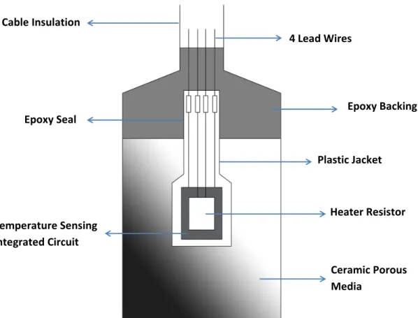
As is shown in Figure 11 (Sattler & Fredlund, 1989), thermal conductivity sensor has a porous ceramic block containing a temperature-sensing element and a miniature heater. To measure soil suction by this method, a hole is drilled in the soil. By putting the sensor in drilled hole, water can flows between the porous block and the soil. After a while, water content of the soil and sensor will equilibrate. Heat dissipation in the block will change by changing amount of water content in porous ceramic block. By measuring this heat dissipation amount of water content can be measured indirectly (Sattler & Fredlund, 1989).

2.1.3 Water Flow in Unsaturated Soil

Generally, a vast knowledge of water flow process in soil is required to study a geotechnical problem. To model water and solute transport in unsaturated soils, it is necessary to hydraulic properties properly. Hydraulic properties are also used for hydraulic classification. This information is necessary for basic understanding of soil hydraulic process.

To select the method for determining soil hydraulic properties, time and expenses are important parameters. Some other parameters like measurement range and accuracy are also concerns to choose the proper technique to find soil hydraulic properties. Regarding these criteria, different methods had been developed to determine or measure soil’s hydraulic properties. Direct and indirect methods are two main categories that can be used to find these properties. Direct methods are usually time consuming and need labor that makes it expensive. To decrease the expenses and the required time to measure these parameters,

(37)

19 4 Lead Wires Epoxy Backing Heater Resistor Plastic Jacket Ceramic Porous Media Temperature Sensing Integrated Circuit Epoxy Seal Cable Insulation

Figure 11: A cross sectional diagram of the thermal conductivity sensor (Sattler & Fredlund, 1989)

some methods were developed to predict soil hydraulic parameters instead of direct measurement. Direct methods rely on measuring the desired hydraulic properties in field or in laboratory. In these methods, parameters like water potential, water flux and water content are measured in soil. Generally, these methods take a longer time and need expensive tools to be performed.

Unsaturated flow process is not easy to describe and formulate. Normally, during the flow in unsaturated media, soil water content changes.

Darcy’s law is the fundamental equation for describing flow in porous material. This equation was presented by Darcy (1856) and relates the flow velocity (𝑞) to the permeability of the medium (𝐾) and the fluid’s inside pressure (𝜓).

(38)

20

𝑣𝑤 = −𝑘𝜕ℎ_𝜕𝑧𝑤 Equation 10

where 𝑣𝑤 is the flow rate of water and k is the coefficient of permeability with respect to the water phase. 𝜕ℎ𝑤⁄ is the hydraulic head gradient in z-direction, where ℎ𝜕𝑧 𝑤 is the total hydraulic head.

By combining Darcy’s law with the continuity equation, Richards (1931) proposed an equation to describe water movement in unsaturated soils. Richards’ equation for one-dimensional z-direction (vertical) flow is as below:

𝜕𝜃 𝜕𝑡 = 𝜕 𝜕𝑧 �𝐾(ℎ) � 𝜕ℎ 𝜕𝑧 + 1�� Equation 11

where 𝐾 is the hydraulic conductivity, ℎ is the pressure head, 𝑧 is the elevation above a vertical datum, 𝜃 is the water content, and 𝑡 is time. Because of the constitutive relationship between ℎ and 𝜃 it is possible to write Richards’ equation either with pressure head or soil moisture form.

This is the basic equation for flow in unsaturated soils. By analytical or numerical solutions of this equation, the soil water content corresponding to a spatial location and a given time can be found. Richards’ equation can be applied to saturated and unsaturated soils. At equilibrium [𝜕ℎ 𝜕𝑧⁄ ] is equal to 1.

In Richards’ equation the [𝜕𝜃 𝜕𝑡⁄ ] term can be replaced by 𝐶(ℎ) ∗ [𝜕ℎ 𝜕𝑡⁄ ] where 𝐶(ℎ) is [𝑑𝜃 𝑑ℎ⁄ ]. Celia et al. (1990) proposed 𝐶(ℎ𝑚) as water capacity function.

Hydraulic conductivity is one the most important hydraulic properties of the soils that effects flow in soil. By solving Richards’ equation using inverse modelling method, hydraulic properties of unsaturated soils can be estimated (Eching et al. 1994; Fujimaki & Inoue 2004; van Dam et al. 1994; Šimůnek et al. 1998). Inverse modelling requires some soil retention data (van Dam et al. 1990). These data can be provided by using experimental

(39)

21 methods. Soil water retention curve which represents relationship between soil suction (𝜓) and volumetric water content (𝜃) can be found by performing some laboratory experiments.

2.2 Hydraulic Properties of Unsaturated Soils

2.2.1 Soil Water Retention Curve

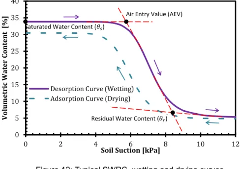
Soil water retention curve (SWRC), which is also called soil water characteristic curve (SWCC) is the relationship between soil suction and soil water content (degree of saturation). Figure 12 (Inspired from Fredlund et al. 1994) illustrates a typical SWRC. In this figure, vertical and horizontal axis show volumetric water content and soil suction, respectively. Air-entry value (AEV), residual water content (𝜃𝑟) and saturated water content (𝜃𝑠) are shown in this figure. Pore space distribution in soil texture has an important role in properties of SWRC.

As is illustrated in Figure 12 (Inspired from Fredlund et al. 1994), water content in the wetting curve is lower than the drying curve for a given matric potential. This behaviour is called hysteresis and affects the SWRC. Hysteresis is a result of entrapped air, contact angles in soil structure, swelling and shrinking and inkbottle effects in soil.

As it is shown in Figure 13 (Fredlund & Xing, 1994), SWRC changes in a wide range for different types of soils. Generally, soils with higher plasticity values have higher saturated volumetric water content and air-entry values (Fredlund & Xing, 1994). Clay has the highest saturated water content compare to silt and sand.

Maqsoud et al. (1975) did some studies on effects of hysteresis on the water retention curve. They performed some tests to study this phenomenon and compared their experimental results with predictive models. They used different types of sands (fine, coarse and silty sand). Their results showed that hysteresis has more effect on fine sands and silty sands compare to coarse sands. Their results also showed that the “Universal Mualem” model cannot predict SWRC adequately. Normally this hysteresis can be neglected in most practical applications. It is also possible to translate wetting or drying SWRC to another by using some techniques (Fredlund et al. 2011).

(40)

22

Figure 13: Typical SWRC for sandy soil, silty soil and clayey soil (Fredlund & Xing, 1994)

Figure 12: Typical SWRC, wetting and drying curves (Inspired from Fredlund et al. 1994)

SWRC is a function of soil suction (capillary pressure) and degree of saturation (water content). To measure the SWRC, it is necessary to measure these two parameters simultaneously. 0 5 10 15 20 25 30 35 40 0 2 4 6 8 10 12 Vo lu m etr ic W ate r C on te nt [% ]

Soil Suction [kPa] Desorption Curve (Wetting)

Adsorption Curve (Drying)

Air Entry Value (AEV) Saturated Water Content (𝜃𝑠)

(41)

23 2.2.1.1 Measuring the Soil Water Retention Curve

To measure the soil water retention curve, water content for corresponding soil suction should be known at different suction values. Generally, the test procedure involves a soil sample on top of a saturated membrane or a porous plate. Pairs of volumetric (or gravimetric) water content and suction values are obtained when the water in the sample is in equilibrium with the water the reservoir. SWRC can be obtained by plotting these values. The method that is used to measure these pair values can involve wetting or drying procedures. As it was mentioned earlier, the procedure to obtain SWRC is hysteretic (Maqsoud et al. 1975; Šimůnek et al. 1999). Because of that, the SWRC obtained for a given pressure head in the wetting process is normally less than the one that is obtained by drying process.

2.2.1.1.1 Axis Translation Technique

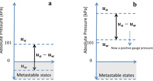
Cavitation is a phenomenon that can happen when the water pressure is relatively low. In soil science, cavitation is a problem that can happen when negative pore water pressure reaches zero. In measuring the soil water retention curve, the soil sample can be filled by air bubble when cavitation happens. Methods based on this technique, beside the hanging water column, are the common methods of studying hydraulic properties of unsaturated soils. Marinho et al. (2008) and Vanapalli et al. (2008) discussed the axis translation technique as a method to control suction in unsaturated soils. In this technique, the cavitation related to pressures greater than 100 kPa is eliminated by using a new procedure. The same amount of pressure is subjected to pore air and pore water pressures since the matric suction, (𝑢𝑎− 𝑢𝑤), will remain the same. The principle of the axis translation technique is shown in Figure 14 (Marinho et al., 2008). In this figure, matric suction is more than 100 kPa. This can cause metastable state in atmospheric pressure. To prevent this phenomenon, sample can be subjected to a large positive air pressure. In this condition, higher pore water pressures can be applied to the soil sample for the same matric suction value without being in metastable state ( Marinho et al. 2008).

(42)

24

Figure 14: Use of the axis translation technique to avoid metastable states (a) Atmospheric conditions (b) axis- translation (Marinho et al. 2008)

Axis translation technique can be used in a pressure plate apparatus or a Tempe Pressure Cell to measure soil water retention curve. Leong et al. (2004) and Wang and Benson (2004) described the design of pressure plate apparatus for measuring soil water retention curve. Wildenschild et al. (1997), Fujimaki & Inoue (2004) and Eching & Hopmans (1993) are some of the researchers who used axis translation technique to measure soil water retention curve.

2.2.1.1.2 Hanging (Negative) Water Column

Hanging column water that was originally proposed by Haines (1927, 1930) is proper for suctions between 0-80 kPa. This test is generally performed in a Buchner funnel. In Figure 15 (ASTM-D6836–02, 2012), a funnel is shown. Specimen chamber, an outflow measurement tube and a suction supply are three main parts of a hanging water apparatus. A schematic view of hanging water column apparatus is given in Figure 16 (ASTM-D6836–02, 2012). To perform the test, a manometer is used to measure the amount of applied suction. A capillary tube which is connected to the outlet of the funnel is used to measure the amount of the extracted water from the specimen while the test is running

Ab so lu te P res su re [ kPa]

a

𝒖

𝒂

𝒖

𝒘

𝒖

𝒂

− 𝒖

𝒘 0 101 Metastable states Ab so lu te P res su re [ kPa]

b

𝒖

𝒂

𝒖

𝒘

𝒖

_𝒂

− 𝒖

_𝒘 0 101 Metastable states

(43)

25 (ASTM-D6836–02, 2012). The gas pressure that is applied to the sample is at atmospheric pressure (𝑃𝑎𝑡𝑚, 𝑃𝑎). Bulk water has sub-atmospheric pressure levels. This pressure can be provided by reducing the level of water in the reservoir or by decreasing the controlled gas pressure 𝑃𝑔. Gas can be dissolved from the bulk water, which can cause a problem in this test. Because of this fact, the suction apparatus has a minimum value which is -85 kPa at elevations near sea level (Dane & Topp, 2002).

In this test after reaching the desired matric suction, the final volumetric water content should be determined. To determine 𝜃, the soil sample should be removed and after weighting should be place in an oven for about 48 hours at 105 °C, so:

𝜃 = (𝑀1− 𝑀2)/𝜌𝑉 Equation 12

where 𝜃 is the volumetric water content. 𝑀1 and 𝑀2 are the soil mass before and after placing in the oven, respectively. 𝜌 is the density of water and 𝑉 is the volume of soil sample.

2.2.1.1.3 Pressure Plate Extractor

Hanging water column and pressure cell have an important limit that is related to their applicable minimum suction value that is equal to -8.5 m. Pressure plate extractor is a method that was developed for high suction values (Dane & Topp, 2002). To perform a test in high pressures with this method, a high air-entry porous ceramic plate is necessary. These ceramics are made of mixture of ball clays and are manufactured by a sintering process. During the test, these ceramics separate the air and the water phase (Leong et al. 2004).

(44)

26

Figure 15: Photograph of a funnel used for hanging column apparatus (ASTM-D6836–02, 2012)

Pressure plate extractors are also called pressure plates. This apparatus can be used to determine soil water content in drying or wetting process. The procedure of this method can be found in “Methods of Soil Analysis” (Dane & Topp, 2002). Figure 17 (Soilmoisture Equipment Corp.) shows a 5-bar Pressure plate extractor. From 5 to 8 soil samples can be inserted on the ceramic plate in different models. This ceramic plate is normally supported by a pressure chamber that is equipped with some valves for air pressure inlet and an air release valve.

By using a pressure regulation system, air pressure can be applied to the system and water can flow out of the pressure chamber. When there is no more flow for a given pressure, the final water content of each sample can be determined weighing the sample. This is repeated for different pressure values to have pairs of suction and water content.

(45)

27 Figure 16 : Schematic view of a hanging column apparatus

(ASTM-D6836–02, 2012)

Figure 17 : 5 Bar Pressure Plate Extractor, picture from Soilmoisture Equipment Corp. (soilmoisture.com)

(46)

28

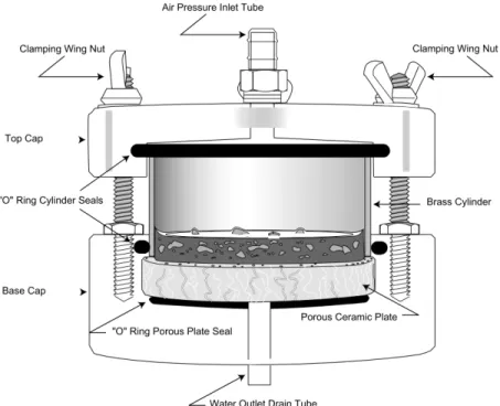
Figure 18: Cross sectional view of the sketch of a Tempe Cell (Soilmoisture Equipment Corp. 1995)

2.2.1.1.4 Tempe Pressure Cell

Tempe pressure cell is an apparatus that can be used to measure the soil water characteristic curve. This apparatus can be used for coarse and fine-grained soils. In this method an individual core of the soil sample is inserted on top of a porous ceramic plate. An air pressure inlet on top of the cell is used to apply pressure to the soil sample. This apparatus can be used for pressures between 0 to -100 kpa to prevent depressurization phenomena. Figure 18 (Soilmoisture Equipment Corp. 1995) shows a cross sectional view of the sketch of a Tempe Cell. The water outlet at the bottom of the cell allows the extracted water to flow towards the reservoir. A regulated gas pressure source is required to apply high pressures to the soil sample. Due to the pressure inside the soil sample, water will be extracted. Extracted water for each pressure value can be recorded and used to determine soil water retention curve with this method. This test can be performed in one-step or in multiple pressure steps. By performing this test in multiple steps, applied pressure increases in multiple steps and the extracted water value is measured for each pressure value.

(47)

29 Figure 19: Some common soil water content measurement methods and

their corresponding matric suction ranges (Tuller & Or, 2003)

In Figure 19 some methods of measuring SWRC and their corresponding matric suctions are given. Each method is suitable for a certain range of matric suction; for example, the psychrometer is better for higher matric suction values and the Tempe Cell is suitable for lower matric suctions.

2.2.1.2 Modelling Soil Water Retention Curve

It is time consuming and difficult to measure SWRC in laboratory. Different mathematical models were introduced by different peoples to represent SWRC based on their other properties. Some of these models are explained later in this chapter. Some of these models use soil’s grain size distribution to estimate soil water retention curve.

2.2.1.2.1 Brooks and Corey

Brooks and Corey (1964) introduced a semi-empirical method to find unsaturated soils hydraulic properties. Brooks and Corey (BC) method gives better results for soils with coarse grain structure. As is it seen in Equation 13, for matric suctions (𝜓) smaller than air-entry value (AEV), the effective degree of saturation (𝑆𝑒) is equal to 1. If the matric suction

Soil Water Content

M at ric S uct ion [-cm] 𝟏𝟎𝟓 𝟏𝟎𝟒 𝟏𝟎𝟑 𝟏𝟎𝟐 𝟏𝟎𝟏

𝜽

𝒓

𝜽

𝒔

(48)

30

is greater than the AEV, 𝑆𝑒 is found by using a correlation that is a function of matric suction and a dimensionless parameter (𝜆). 𝜆 is a constant that characterize pore size distribution and is called pore size distribution index.

𝑆𝑒 = 1 𝑤ℎ𝑒𝑛 𝜓 < 𝜓𝐴𝐸𝑉 𝑆𝑒 = (𝜓𝐴𝐸𝑉_{𝜓 )}𝜆 𝑤ℎ𝑒𝑛 𝜓 ≥ 𝜓𝐴𝐸𝑉 Equation 13 and 𝑆𝑒 = _𝜃𝜃 − 𝜃𝑟 𝑠− 𝜃𝑟 Equation 14

where 𝜃 the volumetric water is content, 𝜃𝑟 is the residual water content and 𝜃𝑠 is the water content at saturation. Equation 13 can be re-written as:

𝜃 = 𝜃𝑠 𝑤ℎ𝑒𝑛 𝜓 < 𝜓𝐴𝐸𝑉 Equation 15

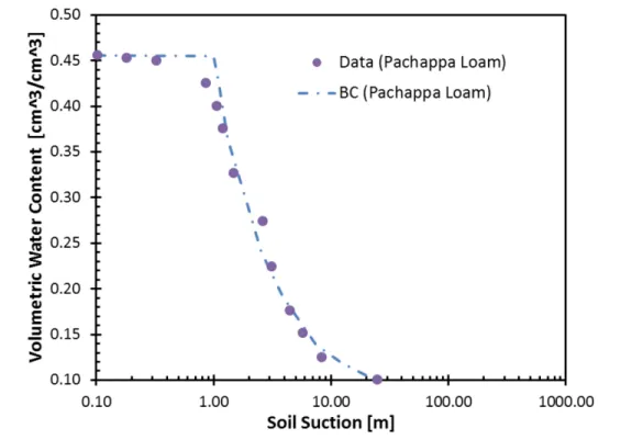
𝜃 = 𝜃𝑟+ (𝜃𝑠 − 𝜃𝑟)(𝜓𝐴𝐸𝑉_{𝜓 )}𝜆 𝑤ℎ𝑒𝑛 𝜓 ≥ 𝜓𝐴𝐸𝑉 Equation 16 where 𝜆 is the pore size distribution index. Figure 20 shows a comparison of SWRC results between Brooks and Corey (BC) model and experimental data for Pachappa loam (Assouline & Tartakovsky, 2001). As is shown in Figure 20, BC curve is formed of a straight line representing saturated part and a slope representing unsaturated part.

2.2.1.2.2 Arya and Paris

Arya and Paris (1981) proposed the first physico-empirical model to predict the SWRC by using particle size distribution and bulk density data. This model was developed for nonswelling soils with low degree of aggregation. They divided soil size distribution to several fractions and assumed that the bulk density of each fraction is equal to the bulk density of natural-structure soil. Based on this assumption they could find pore volume

(49)

31 related to each soil segment by using Equation 17. They approximated the solid volume to the volume of uniform size spheres, which is equal to mean particle radius for the segment and its pore volume is equal to uniform size cylindrical tube with diameter of the mean particle radius for that segment. By these assumptions, they could use Equation 23 to compute the pore radii. They translated particle size distribution into pore size distribution and used capillarity equations to find soil water pressure regarding to each pore radius (Arya & Paris, 1981). In this method pore volume (𝑉𝑣𝑖) is equal to:

𝑉𝑣𝑖 = �𝑊_𝜌𝑖 𝑝� ∗ 𝑒

Equation 17

where 𝑊𝑖 is the solid mass per unit sample mass in the i-th particle size range, 𝜌𝑝 is the particle density and 𝑒 is the void ratio and is equal to:

𝑒 =(𝜌𝑠_𝜌− 𝜌𝑏)

𝑏 Equation 18

where 𝜌𝑠 and 𝜌𝑏 are particle and bulk densities, respectively.

Average volumetric water content of the midpoint of the i-th particle size range can be obtained as follows: 𝜃𝑣𝑖 = �𝑉_𝑉𝑣𝑗 𝑏 𝑗=𝑖 𝑗=1 ; 𝑖 = 1,2, … , 𝑛 Equation 19 𝑉𝑏 = �𝑊_𝜌𝑖 𝑏 𝑖=𝑛 𝑖=1 =_𝜌1 𝑏; 𝑖 = 1,2, … , 𝑛 Equation 20 𝜃𝑣𝑖∗ = (𝜃𝑣𝑖+ 𝜃𝑣 𝑖+1) 2⁄ Equation 21

where 𝜃𝑣𝑖∗ is the average volumetric water content of the midpoint of a given (i-th) particle size range.

(50)

32

By using capillary correlation, suction related to each radius can be determined. The soil water pressure head 𝜓𝑖 can be found with Equation 22.

𝜓𝑖 = 2𝑇𝑠 𝑐𝑜𝑠𝛼/𝜌𝑤𝑔𝑟𝑖 Equation 22

where 𝑇𝑠 is the surface tension of water, 𝛼 is the contact angle, 𝜌𝑤 is the density of water, 𝑔 is the gravity and 𝑟𝑖 is the pore radius and 𝑟𝑖 is equal to:

𝑟𝑖 = 𝑅𝑖�4𝑒𝑛𝑖(1−𝛽)/6�1/2 Equation 23

where 𝑟𝑖 is the mean pore radius, 𝑅𝑖 is the mean particle radius, 𝑛𝑖 is the number of particles, and 𝛽 is an empirical constant.

Arya and Paris set 𝜃 to 0 for t=25o _{C, but if the contact angle can be used to adjust the}

results, if it is defined. To predict SWRC of aggregates, it was suggested to use aggregate size distribution in addition to particle size distribution. Results of Arya and Paris model shows a good agreement with measured data for several soils, but there is a considerable disagreement between measured and model values for some other soils (Arya & Paris, 1981). Figure 21 shows a comparison between Aria and Paris (1981) model measured data SWRC values for two Jersey soils. As is seen, there is a good agreement between predicted and measured data for these soils (Arya & Paris, 1981).

2.2.1.2.3 Fredlund and Xing (1994)

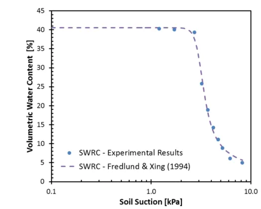
Fredlund and Xing (1994) proposed a new model for SWRC. They assumed that at suction equal to 1000 000 kPa, soil will be completely dry and the water content is 0. This equation was based on the assumption that the shape of the SWRC is dependent on the pore size distribution.

𝜃 = 𝜃𝑠 𝐶(𝜓) �_{𝑙𝑛[𝑒 + (𝜓 𝑎}1 _{⁄ )}_𝑛_]� 𝑚

Equation 24

where 𝑎, 𝑛 and 𝑚 are fitting soil parameters, 𝑒 is the Napier's constant, 𝜓 is the soil suction and 𝐶(𝜓) is a correction factor which is equal to:

(51)

33 𝐶(𝜓) = �1 −_{𝑙𝑛(1 + 1000000 𝜓}𝑙𝑛 (1 + 𝜓 𝜓⁄ )𝑟

𝑟

⁄ )� Equation 25

where 𝜓𝑟 is the residual soil suction.

In Figure 22 an example of applying Fredlund and Xing (1994) model to obtained experimental data is shown. As it is seen, the fitted curves are in a close agreement with the experimental data over the entire suction range.

Figure 20 : Comparison of SWRC results between Brooks and Corey and data for Pachappa loam (Assouline & Tartakovsky, 2001)

(52)

34

Figure 21 : Comparison between measured data and Aria and Paris (1981) model predicted values of SWRC for two Jersey soils (Arya & Paris, 1981)

(53)

35 2.2.1.2.4 van Genuchten (1980)

van Genuchten (1980) proposed new equations for SWRC. This model is applicable to different types of soils. By fitting van Genuchten (1980) model (VG) to the experimental data, three independent fitting parameters are obtained.

𝑆𝑒 = [1 + |𝛼𝜓|𝑛]−𝑚 _{Equation 26}

𝑆𝑒 = _𝜃𝜃 − 𝜃𝑟 𝑠− 𝜃𝑟

Equation 27

where 𝑆𝑒 is the effective saturation, 𝛼 ( > 0) is a function of the inverse of the air-entry pressure, 𝑛 ( >1 ) is a function of pore size distribution and 𝑚 = 1 − 1/𝑛. 𝜓 is the soil suction and 𝜃 is the volumetric water content and 𝜃𝑟 and 𝜃𝑠 are the residual and saturated

Figure 22 : A Fredlund & Xing (1994) model best-fit curve to the experimental data of a sandy material

(54)

36

water contents, respectively. By combining Equation 26 and Equation 27, volumetric water content can be found as:

𝜃 = 𝜃𝑟+ (𝜃𝑠 − 𝜃𝑟) �_{1 + (𝛼𝜓)}1 _𝑛� 𝑚

Equation 28

To measure the suction by having the water content values, Equation 28 can be re-arranged as below: 𝜓 = 1 𝛼 �� 𝜃 − 𝜃𝑟 𝜃𝑠− 𝜃𝑟� −1 𝑚� − 1� 1 𝑛� _{Equation 29}

By replacing 𝑚 with 1 − 1/𝑛 as was suggested by Mualem (1976) fitting parameters will drop to two and the new equation will be re-written as below”

𝜃 = 𝜃𝑟+ (𝜃𝑠 − 𝜃𝑟) �_{1 + (𝛼𝜓)}1 _𝑛�

(1−_𝑛1) _{Equation 30}

In Figure 26-a, an example of applying van Genuchten model to Hygiene Sandstone experimental data (data from: Brooks & Corey, 1964) is shown. As it is seen, this model has a very good agreement with experimental data.

2.2.2 Hydraulic Conductivity of Unsaturated Soils

Hydraulic conductivity describes the capacity of the soil to transmit water. According to the Kozeny-Carman equation (Equation 31) hydraulic conductivity of saturated materials is affected by different parameters. This equation can be described as below (Carrier, 2003):

𝐾 = 1 𝐶𝑆02 𝛾 𝜇 𝑒3 (1 + 𝑒) Equation 31

where K is the saturated hydraulic conductivity, γ is the unit of weight of permeant, μ is the viscosity of the permeant, 𝑒 is the void ratio, 𝐶 is the Kozeny-Carman empirical coefficient and 𝑆0 is specific surface area per unit volume of particles �_𝑐𝑚1 �.

(55)

37 Hydraulic conductivity decreases by decreasing soil unit weight. Soil temperature is another parameter that affects hydraulic conductivity of saturated materials. Void ratio, particle size, composition, fabric structure and degree of saturation also have influence on hydraulic conductivity of saturated materials. Soils with higher void ratio have higher hydraulic conductivity. 𝐷10 is inversely proportional to 𝑆0. From Equation 31 it is evident that 𝑆0 is inversely proportional to 𝐾, which implies 𝐷10 and 𝐾 are directly proportional. Soils with bigger particles have higher permeability.

One of the properties of the soils that has a great influence on hydraulic conductivity of coarse-grained soils is the percentage of fine particles (Passing from No. 200 sieve). Existence of chemicals in fluids can also have some influences on hydraulic conductivity (Sharma & Lewis, 1994).

Darcy’s law (Equation 10) defines hydraulic conductivity for saturated materials. Richards proposed an equation by applying Darcy’s law for unsaturated soils. Hydraulic conductivity in unsaturated zone can be expressed in a relation with soil suction (𝜓) or soil water content (𝜃). By increasing soil suction, hydraulic conductivity in soil decreases. Hydraulic conductivity of soils in unsaturated zone can be measured or estimated by different direct and indirect methods. To select the proper method for finding hydraulic conductivity, different parameters have to be considered. Time, cost, existence of equipment, skill of the staff who perform the test and type of the soil are some of these parameters. Different laboratory and field techniques were developed to measure hydraulic conductivity of unsaturated soils. Measuring methods are usually expensive and time consuming. Due to these problems, different attempts were done to find hydraulic conductivity by using indirect methods that are usually cheaper and faster than direct methods. Some methods of determining hydraulic conductivity of unsaturated soils are explained later in this chapter. 2.2.2.1 Direct Methods

Various direct methods were proposed by different researchers to measure hydraulic conductivity of unsaturated soils in field and laboratory. Steady state methods and unsteady

(56)

38

state methods are two major groups of direct methods of measuring hydraulic conductivity of unsaturated soils.

In steady state methods of determining unsaturated hydraulic conductivity 𝐾(𝜃), volumetric flux density and the hydraulic gradient are measured at given water content. A series of steady state flows are established and water flux and hydraulic gradient are recorded for each given water content value. The corresponding hydraulic conductivity for each 𝜃 value will be found by flux and hydraulic gradient data and using Equation 10, which is a finite –difference form of Darcy’s equation.

Corey (1957, Cited by Masrouri et al. 2008) proposed a steady state method to find hydraulic conductivity of soils as a function of water content. He used a long column with some tensiometers which were installed on its wall. In this method, to have the hydraulic conductivity as a function of water content, a procedure should be done to measure water content as a function of soil suction. In this method for each step water will be entered form the top of the column (if wetting process is chosen) at a small steady rate. This will be continued till a steady flow into the column is reached and water content in the cell is constant. Therefore, the conductivity corresponding to that specific water content will be the same as flow rate for that step.

The most important limitation of this method is its necessity for a long homogenous soil column; so this method cannot be used for disturbed soil samples (Hopmans et al. 2002). Beside proposed steady state methods, some researchers proposed unsteady methods to measure hydraulic conductivity of unsaturated soils. Instantaneous profile method (IPM) and Inflow-Outflow method are some of unsteady state methods.

Rose et al. (1965) was the first who developed the IPM method. This method is based on measuring hydraulic conductivity of soils for several depths as a function of water content. This method was then used and developed by some researchers like Watson (1966) and Chiu and Shackelford (1998) for determining the hydraulic conductivity of unsaturated materials.

(57)

39 Gypsum crusts were used by Bouma and Denning (1972) to find unsaturated soils hydraulic conductivity in field. To measure hydraulic conductivity of the soil by this method, a cylinder is made on soil surface. A mixture of gypsum and coarse sand is prepared. This mixture will be poured over that cylinder’s surface. A flux is applied over the gypsum to have a constant head. Water potential at the bottom of the gypsum crust is measured by tensiometers. By measuring this flux rate and the diameter of the cylinder, hydraulic conductivity can be determined (ASTM-Standard-D5126).

2.2.2.1.1 Evaporation

Evaporation method is one of the laboratory methods that can be used to determine SWRC and unsaturated hydraulic conductivity at the same time. This method was introduced by Gardner and Miklich (1962, Cited by Šimůnek et al. 1998). They imposed different evaporation rates to the sample. Each new rate was applied after equilibrium of the sample. The most popular procedure that is used to find hydraulic properties of the soils by evaporation method is a result of Wind (1966) efforts. He used a vertical cylinder filled with undisturbed soil material that was saturated with water. Sample was allowed to

Figure 23 : Schematic view of a centrifuge permeameter with relevant variables (Reprinted from Zornberg & McCartney, 2010)

(58)

40

evaporate only on its top. Wendroth et al. (1993) proposed an evaporation method to find soil hydraulic conductivity function and the water retention characteristic. They used a 6.0

cm high soil column and used two pressure tensiometers which were installed at 1.5 cm and

4.5 cm form the bottom of the cell. Top of the column was open, so the water could evaporate (Figure 24). They used numerical simulation to find hydraulic functions.

2.2.2.2 Indirect Methods

Measuring unsaturated hydraulic conductivity by using direct methods is expensive and time consuming. Because of this problem, some indirect methods were developed to find hydraulic conductivity of unsaturated soils. Most of these methods use saturated hydraulic conductivity and SWRC to find hydraulic conductivity unsaturated soils.