HAL Id: pastel-00576471
https://pastel.archives-ouvertes.fr/pastel-00576471
Submitted on 14 Mar 2011HAL is a multi-disciplinary open access
archive for the deposit and dissemination of sci-entific research documents, whether they are pub-lished or not. The documents may come from teaching and research institutions in France or abroad, or from public or private research centers.
L’archive ouverte pluridisciplinaire HAL, est destinée au dépôt et à la diffusion de documents scientifiques de niveau recherche, publiés ou non, émanant des établissements d’enseignement et de recherche français ou étrangers, des laboratoires publics ou privés.
Quelques Contributions au Traitement de Signal Musical
et à la Séparation Aveugle de Source Audio
Mono-Microphone
Antony Schutz
To cite this version:
Antony Schutz. Quelques Contributions au Traitement de Signal Musical et à la Séparation Aveugle de Source Audio Mono-Microphone. Traitement du signal et de l’image [eess.SP]. Télécom ParisTech, 2010. Français. �pastel-00576471�
THESE
pr´esent´ee pour obtenir le grade de
Docteur de TELECOM ParisTech Sp´ecialit´e: Signal et Image
Antony Schutz
Quelques Contributions au Traitement de
Signal Musical et `
a la S´
eparation Aveugle
Mono-Microphone de Source Audio
Th`ese soutenue le 2 D´ecembre 2010 devant le jury compos´e de :
Pr´esident Ga¨el Richard TELECOM ParisTech
Rapporteurs Olivier Michel INPG
Fr´ed´eric Bimbot CNRS-INRIA
Examinateurs Nicholas Evans EURECOM
Mahdi Triki Philips
DISSERTATION
In Partial Fulfillment of the Requirements for the Degree of Doctor of Philosophy
from TELECOM ParisTech
Specialization: Signal and Image
Antony Schutz
Some Contributions to Music Signal
Processing and to Mono-Microphone
Blind Audio Source Separation
Thesis defensed on the 2nd of December 2010 before a committee composed of:
President Ga¨el Richard TELECOM ParisTech
Reporters Olivier Michel INPG
Fr´ed´eric Bimbot CNRS-INRIA
Examiners Nicholas Evans EURECOM
Mahdi Triki Philips
i
R´
esum´
e
Pour les ˆetres humains, le son n’a d’importance que pour son contenu. La voie est un lan-gage parl´e, la musique une intention artistique. Le processus physiologique est hautement
d´evelopp´e, tout comme notre capacit´e `a comprendre les processus sous-jacent. C’est un
d´efi de faire ex´ecuter la mˆeme tˆache `a un ordinateur: ses capacit´es n’´egalent pas celles
des humains lorsqu’il s’agit de comprendre le contenu d’un son compos´e de paroles et/ou d’instruments de musique. Dans la pr´esente th`ese nous avons envisag´e deux des aspects
reli´es `a cette probl´ematique: la s´eparation aveugle de source ainsi que le traitement
mu-sical. Dans la premi`ere partie nos recherches portent sur la s´eparation aveugle de source en n’utilisant qu’un seul microphone. Le probl`eme de s´eparation de source audio ap-paraˆıt d`es que plusieurs sources audio sont pr´esentes au mˆeme moment, m´elang´ees puis acquises par des capteurs, un unique microphone dans notre cas. Dans ce genre de situ-ation il est naturel pour un ˆetre humain de s´eparer et de reconnaˆıtre plusieurs locuteurs.
Ce probl`eme, connu sous le nom de Cocktail Problem `a re¸cu beaucoup d’attention mais
est toujours ouvert. Dans cette partie nous pr´esentons deux types d’algorithmes afin de r´esoudre ce probl`eme. Comme nous ne travaillons qu’avec une seule observation nous ne
pouvons pas utiliser d’indice li´e `a la spatialisation et nous sommes dans l’obligation de
mod´eliser les sources. Nous utilisons un mod`ele param´etrique dans lequel une source est repr´esent´ee comme ´etant la r´esultante de deux processus autor´egressifs, de longueur de corr´elation diff´erentes, en cascade et excit´es par un bruit blanc Gaussien, la mixture est la somme de ces sources plus un bruit blanc Gaussien. Les signaux ´etant non stationnaires, le premier type d’algorithme propos´e suit une m´ethodologie adaptative. Le deuxi`eme type d’algorithme, lui, analyse l’observation par morceaux en consid´erant une station-narit´e locale. Dans ce contexte la s´eparation se passe en deux ´etapes, tout d’abord les param`etres sont estim´es dans le m´elange puis ils sont utilis´es afin d’effectuer la s´eparation. La deuxi`eme partie traite du traitement musical et est compos´ee de plusieurs annexes. La tˆache analys´ee est li´ee au traitement automatique de la musique, qui a pour but de com-prendre un contenu musical afin d’en g´en´erer la partition. Cependant la musique ne peut
pas ˆetre r´eduite `a une succession de notes et un bon transcripteur devrait ˆetre capable
de d´etecter les effets d’interpr´etations et la qualit´e de jeu du musicien. Les outils con¸cus peuvent ´egalement ˆetre utilis´es dans un but p´edagogique pour aider un apprenti musicien `
a am´eliorer ses comp´etences. Dans cette partie nous avons port´e attention `a la d´etection
de certains effets et d´efaut de jeu. Puis nous proposons une m´ethode afin de d´etecter la pr´esence de l’octave lorsqu’elle est jou´ee avec sa fondamentale. Comme l’octave d’une note a une fr´equence double de sa fondamentale, elles partagent les mˆemes pics fr´equentiels et la d´etection est ardue. Nous proposons un crit`ere bas´e sur le rapport d’´energie des pics fr´equentiels pairs et impairs pour faire la d´etection. Finalement cette partie se termine avec la description d’un transcripteur Audio-Visuel de Guitare dont le but est de fournir une tablature et non une partition.
iii
Abstract
For humans, the sound is valuable mostly for its meaning. The voice is spoken language, music, artistic intent. Its physiological functioning is highly developed, as well as our understanding of the underlying process. It is a challenge to replicate this analysis using a computer: in many aspects, its capabilities do not match those of human beings when it comes to speech or instruments music recognition from the sound, to name a few. In this thesis, two problems are investigated: the source separation and the musical processing.
The first part investigates the source separation using only one Microphone. The problem of sources separation arises when several audio sources are present at the same moment, mixed together and acquired by some sensors (one in our case). In this kind of situation it is natural for a human to separate and to recognize several speakers. This problem, known as the Cocktail Problem, receives a lot of attention but is still open. In this part we present two algorithms for separating the speakers. Since we work with only one observation, no spatial informations can be used and a modelization of the sources is needed. We use a parametric model for constraining the solution: a mixture is modeled as a sum of Autoregressive sources with an additive white noise. The sources are themselfs modeled by a cascade of two AR model with differents correlation lenghts. The first algorithm is adaptive, for a non stationary signal it is natural to want to follow the variation of the signal over the time. The second algorithm works with consecutive frames of short duration. The procedure is splitted in two parts: first an estimation of the sources parameters is done on a frame, then a non iterative separation algorithm is used. Finally the estimated parameters are used for the initilization of the next analysed frame.
The second part deals with Musical Processing and is composed of several annexe. The task that we investigate is connected to the Automatic Music Transcription task, which is the process of understanding the content of a song in order to generate a music score. But, music cannot be reduced to a succession of notes, and an accurate transcriptor should be able to detect other performance characteristics such as interpretations effects. The tools built for automatic transcription can also be used in a pedagogic way, so that even a student can improve his performances with the help of a software. This means that the software should be able to detect some interpret’s flaws. In this part, first of all we collect several samples of interpretation effects and performing defects. Then, we have built some tools for finding the presence (or not) of the considered effect. Another problem in music transcription is called the octave problem, it appears when a note and its octave are present together. As the octave has a frequency twice the note, they share the periodicity and the partials of the spectrum are perfectly overlapped. This makes the detection laborious. We propose an energetic criterion based on the estimation of the energy of the odd and even partials of the chord. Finally, the last chapter deals with the description of an audio-video simulator specialized for writing guitar tablature instead of partition.
v
Acknowledgements
I would like to thank particularly Professor Dirk T.M Slock, my thesis supervisor, for so many things that it is impossible to list them all. First of all he gave me the opportunity to do a PhD with him and in EURECOM, a very special place. He was also very supportive during some hard moments. I will never forget some dinners, around a good bottle of wine and luscious food. He allowed me to work, at my own pace, on challenging topics and to assist him in several projects, students’ project and courses management. I also thank him for his guidance during the years I spent at EURECOM.
I am truly grateful to Professor Olivier Michel and to Fr´ed´eric Bimbot for accepting to be the reporters of my thesis and for all the feedback they gave me for improving my work. I also thank the president Professor Ga¨el Richard that I met several times during project meeting. I finally thank Nicholas Evans and Mahdi Triki (my elder brother) for being examiners.
I would like to thank David, Bassem, Lorenzo, Daniel, Turgut and specially Stephanie for their help for this manuscript. I also thank people with whom I had collaborations, as Henri, Eric, Sacha, Marco, Benoit, Siouar, Simon, Valentin, Nancy, Roland and Bertrand. My memories about EURECOM are not limited to just scientific research, but also to side activities like organizing conferences and seminars, as well as to social initiatives as being the goal keeper of the EURECOM football team (thanks Seb).
I had the chance to meet great colleagues and collaborators, but mostly, great friends. I especially think about Raul, Nadia, Fadi, Farrukh, Hicham, Jerome and Saad, who wel-come me at EURECOM, as well as those I met later, as Bassem, Marco, Virginia, Randa, Daniel, Erhan, Lorenzo, Zoe, Zuleita, Umer, Turgut, Kostaks and Ikbal. And of course everyone at EURECOM.
I also appreciated to work with EURECOM students for semester projects. For this reason, I give my thanks to Lucia, Valeria, Guillaume and Pierre-Etienne. I also thank Siouar, whom I followed during her Master Project, and who became my little sister. Thanks to all the other colleagues, secretaries and to the IT service.
I will always cherish wonderful memories of these past years at EURECOM.
Last but not the least, I am grateful to my family and my friends, for their sincere love and unconditional support, before, during, and after my PhD studies.
vii
Contents
R´esum´e . . . i Abstract . . . i Acknowledgements . . . v Contents . . . vii List of Figures . . . xv Acronyms . . . xix Notations . . . xxiOverview of the thesis and contributions . . . xxiii
0.1 Thesis Overview . . . xxiii
0.2 Contributions . . . xxv
0.2.1 Blind Audio Source Separation . . . xxv
0.2.2 Annexe: Musical Processing . . . xxvii
R´esum´e des travaux de th`ese . . . xxix
0.3 Introduction `a la s´eparation aveugle de source . . . xxix
0.3.1 Quelques solutions existante . . . xxx
0.3.2 Positionnement du travail expos´e . . . xxxi
0.3.3 La s´eparation aveugle de source Mono-Microphone . . . xxxi
0.4 Mod`ele utilis´e . . . xxxiv
0.4.1 La parole . . . xxxiv
0.4.2 Mod´elisation `a long terme . . . xxxiv
0.4.3 Mod´elisation `a court terme . . . xxxv
0.4.4 Mod`ele de source . . . xxxvi
0.4.5 Mod`ele de m´elange . . . xxxvi
0.5 Traitement adaptatif . . . xxxviii
0.5.1 Algorithme de type EM-Kalman . . . xxxviii
0.5.2 Algorithme EM-Kalman adaptatif . . . xxxviii
0.5.3 S´eparation de source Mono-Microphone avec un EM-Kalman . . . . xxxix
0.5.4 Estimation des param`etres et discussion sur les ´etats partiels . . . . xl
0.5.5 R´esultat de simulations sur des signaux synthetiques . . . xli
0.6 Traitement ”par fenˆetre” . . . xlii
0.6.1 Distance d’Itakura Saito . . . xlii
0.6.2 Interpr´etation Na¨ıve de la distance IS . . . xlii
0.6.2.1 Estimation de param`etres par la m´ethode Na¨ıve . . . xliii
0.6.3 Minimisation de la distance IS . . . xliii
0.6.4 Algorithme de s´eparation de source . . . xliv
0.6.4.1 Mod`ele conjoint . . . xliv
0.7 Simulations . . . xlvi
viii CONTENTS
0.7.2 Signaux de longue dur´ee: Parole . . . xlvii
0.7.3 Signaux de longue dur´ee: Musique . . . xlix
0.7.4 Discussion des performances . . . l
0.7.5 Extraction du bruit de fond . . . li
0.7.5.1 param`etres utilis´es . . . lii
0.8 Conclusions . . . liii
0.9 Perspectives . . . liv
I Mono-Microphone Blind Audio Source Separation 1
1 Introduction 3
1.1 Blind Source Separation . . . 4
1.1.1 Introduction . . . 4
1.1.2 Determination . . . 4
1.1.3 Effect of the propagation . . . 5
1.2 Application . . . 5 1.2.1 Audio Processing . . . 5 1.2.2 Biomedicine . . . 6 1.2.3 Diarization . . . 6 1.2.4 Security . . . 6 1.2.5 Telecommunications . . . 6
1.3 Some existing solutions . . . 7
1.3.1 A brief Chronology . . . 7
1.3.2 Determined and Over determined BSS . . . 7
1.3.3 Under determined BSS (UBSS) . . . 8
1.3.4 Stereophonic BSS . . . 8
1.4 Positioning of this thesis . . . 9
1.5 Mono-Microphone Blind Audio Source Separation . . . 9
1.5.1 Problem Formulation . . . 9
1.5.2 Factorial vector quantization (VQ) . . . 10
1.5.3 Gaussian Mixture Models (GMM) . . . 10
1.5.4 Hidden Markov Model (HMM) . . . 10
1.5.5 Non-negative Matrix Factorisation (NMF) . . . 11
1.5.6 Structured/Parametrized Model Based Approach . . . 11
1.5.6.1 Sinusoids Plus Noise . . . 11
1.5.6.2 AR/ARMA-based source separation . . . 13
1.6 Model Considerered in this work . . . 14
1.7 Relationship with another approach . . . 14
1.8 Proposed Approach . . . 15
1.9 Summary of chapter 1 . . . 16
2 Model of Speech Production 17 2.1 Introduction . . . 18
2.2 Speech Model Production . . . 18
2.2.1 How to describe Human Voice . . . 18
2.2.2 A speech signal . . . 18
CONTENTS ix
2.2.3.1 Comb Filter . . . 19
2.2.3.2 Formulation of the Long Term Model . . . 20
2.2.3.3 Traditional Long Term Parameters estimation . . . 21
2.2.4 Modeling the Spectral Shape . . . 22
2.2.4.1 Short Term Autoregressive Model . . . 22
2.3 Mixing Short and Long Term Autoregressive Model: A source . . . 23
2.3.1 Modeling and parameters estimation . . . 23
2.3.2 Spectra Comparison . . . 25
2.4 Multiple Source Plus Noise Model . . . 26
2.4.1 Signal Model . . . 26
2.4.2 Spectral Notation . . . 27
2.5 Summary and discussion . . . 29
3 Adaptive EM-Kalman Filter 31 3.1 Kalman Filter (KF) . . . 32
3.2 Expectation Maximization algorithm (EM) . . . 33
3.2.1 Kalman Smoothing With the EM Algorithm . . . 33
3.2.1.1 Fixed Interval Smoothing . . . 33
3.2.1.2 Fixed lag Smoothing . . . 34
3.3 Adaptive EM-KF with Fixed-Lag Smoothing . . . 34
3.4 Adaptive EM-KF for Mono-Microphone BASS . . . 35
3.4.1 Introduction . . . 35
3.5 State Space Model Formulation . . . 35
3.6 Algorithm . . . 38
3.6.1 Partial states discussion . . . 38
3.6.2 Parameters estimation . . . 39
3.7 Other Approaches using Kalman Filter . . . 41
3.8 Simulations - Synthetic Signals . . . 42
3.8.1 Used parameters to generate synthetic signals . . . 42
3.8.2 Comparison of Models . . . 42
3.8.2.1 Filtering results comparison . . . 43
3.8.2.2 Estimation results comparison . . . 44
3.8.3 Amplitudes tracking . . . 46
3.8.4 Periods Variations . . . 47
3.9 Summary of Chapter 3 and discussion . . . 49
4 Frame Based Source Separation 51 4.1 Frame Based Algorithm . . . 52
4.1.1 Introduction . . . 52
4.1.2 Windowing . . . 52
4.1.2.1 Perfect Reconstruction . . . 53
4.1.3 Related work . . . 53
4.2 Parameters and Sources estimation . . . 54
4.2.1 EM Like Algorithm . . . 54
4.2.2 VB-EM Like Algorithm . . . 54
4.2.3 Proposed Approach . . . 55
4.3 Model . . . 56
x CONTENTS
4.3.2 Set of Parameters . . . 58
4.4 Parameters Estimation Using The Itakura-Saito (IS) Distance . . . 58
4.4.1 Definition of the IS Distance . . . 58
4.4.2 IS Distance for the model . . . 59
4.5 Naive Interpretation of the IS distance . . . 59
4.5.1 Algorithm . . . 59
4.5.1.1 Short term parameters estimation . . . 60
4.5.1.2 Long term parameters estimation . . . 60
4.5.1.3 Noise variance . . . 61
4.6 Minimization of the IS distance . . . 61
4.6.1 Weighted Spectrum Matching . . . 61
4.6.2 Gaussian Maximum Likelihood . . . 61
4.6.3 Short-term AR Parameters Estimation . . . 61
4.6.4 Source Power Estimation . . . 62
4.6.5 Overall iterative process . . . 63
4.6.5.1 A note about the Long Term Model . . . 63
4.7 Parameters Estimation, Synthetic Spectrum . . . 63
4.8 Source Separation Algorithm . . . 64
4.8.1 Joint Source Representation . . . 64
4.8.2 Frequency Domain Window Design . . . 65
4.8.3 Joint Model . . . 67
4.8.4 Estimating the Sources . . . 67
4.8.4.1 Summary of the algorithm . . . 69
4.9 Summary and discussion . . . 69
5 Simulations 71 5.1 Introduction and database details . . . 72
5.1.1 Used Algorithms and initialization details . . . 72
5.2 Short Duration real signals . . . 73
5.2.1 Short Duration real signals, Comparison of Models and orders . . . 76
5.3 Long Duration real signals . . . 78
5.3.1 Filtering Results . . . 79
5.3.2 Estimation Results with Alt-EMK and ”known” periods . . . 81
5.3.2.1 Speech Signals . . . 81
5.3.2.2 Discussion about the simulations and obtained results . . . 83
5.3.2.3 Instrumental Signals . . . 85
5.4 Performances discussion . . . 86
5.5 Vuvuzela remover . . . 88
5.5.1 Procedure and details . . . 88
5.5.2 Results . . . 88
5.6 Summary . . . 90
6 Conclusion 91 6.1 Summary and conclusions . . . 91
CONTENTS xi
II Annexe
Music Signal Processing 95
A Instruments and Interpretation Effects: Description 97
A.1 Introduction . . . 97
A.2 Violin . . . 98
A.2.1 Pizzicato . . . 98
A.3 Electric Bass Guitar . . . 98
A.3.1 Slap . . . 99
A.4 Piano . . . 99
A.4.1 Forte Pedal . . . 99
A.4.2 Practice Pedal . . . 100
A.5 Guitar . . . 100
A.5.1 Palm mute . . . 102
A.5.2 Slide, Bend and Hammer . . . 102
B Tools 103 B.1 Sinusoidal modeling for SNR Estimation . . . 103
B.1.1 Model . . . 103
B.1.2 Motivation, Analysis and synthesis method . . . 104
B.1.3 Estimation - Interpolation - Amplitudes estimation . . . 106
B.1.4 Synthesis, Noise extraction and SNR estimation . . . 109
B.1.5 Discussion on the method . . . 109
B.2 Onset Detection . . . 109
B.2.1 Example of onsets detection . . . 111
B.3 Pitch estimation . . . 112
B.4 Fundamental to Harmonics Energy Ratio (FHER) . . . 113
B.5 Slow variation fondamental frequency tracking . . . 113
B.5.1 Example . . . 114
C Interpretation Effects and Playing Defects: Detection 115 C.1 Violin Playing defects detection . . . 115
C.1.1 Orientation defects . . . 115
C.2 Instruments Interpretation Effects Detection . . . 117
C.2.1 Slap Detection . . . 117
C.2.2 Forte Pedal Detection . . . 119
C.2.2.1 Database . . . 119
C.2.2.2 Feature extraction . . . 120
C.2.2.3 Pre-processing . . . 120
C.2.2.4 Harmonics amplitudes tracking . . . 121
C.2.2.5 Noise estimation . . . 121
C.2.3 Palm mute, Pizzicato and Pratice Pedal detection . . . 124
C.2.3.1 Description . . . 124
C.2.3.2 Palm mute detection result . . . 124
C.2.3.3 Violin Pizzicato . . . 124
C.2.3.4 Pratice Pedal . . . 124
C.2.4 Guitar: Bend, slide and hammer . . . 127
xii CONTENTS
D Periodic Signal Modeling 131
D.1 Problem introduction . . . 131
D.1.1 Illustration . . . 131
D.2 Periodic signal Modeling . . . 133
D.2.1 Definition of the periodic signature . . . 135
D.2.2 As a pitch detector . . . 136
D.2.3 Simulation for the pitch estimation . . . 136
D.2.3.1 Diagram for the pitch determination . . . 137
D.2.3.2 Illustration for the octave determination . . . 137
D.2.4 Application to a true signal . . . 138
D.2.5 Application to the Octave Problem . . . 140
D.2.6 Note plus its Octave . . . 140
D.2.7 Note plus its first two octaves . . . 142
D.2.8 Note plus its second octave . . . 142
D.2.9 Parameters used . . . 143
D.3 Conclusion and Future work . . . 143
E Audio Visual Guitar Transcription 145 E.1 Introduction . . . 145
E.2 Guitar Transcription . . . 146
E.2.1 Automatic Fretboard Detection . . . 146
E.2.2 Fretboard Tracking . . . 147
E.2.3 Hand Detection . . . 147
E.2.4 Audio Visual Information Fusion . . . 148
E.3 Prototype . . . 149
E.4 Future Work . . . 150
E.5 Conclusions and Future work . . . 151
F Miscellaneous 153 F.1 Short Term AR Coefficients Generation Using Levinson Algorithm . . . 153
F.2 Iterative Algorithm for estimating Short plus Long Term AR Model . . . . 154
F.2.1 Short Term AR Coefficients . . . 154
F.2.2 Long Term AR Coefficient . . . 154
F.2.3 Iterative estimation . . . 155
F.3 Short Term Fourier Transform (STFT) . . . 155
F.4 Evaluation Criteria . . . 155
F.4.1 Decomposition . . . 155
F.4.2 Global Criteria . . . 156
F.4.2.1 Source to Distortion Ratio . . . 156
F.4.2.2 Source to Interferences Ratio . . . 156
F.4.2.3 the Sources to Artifacts Ratio . . . 156
F.4.3 Local Criteria . . . 156
F.5 Windows Properties . . . 157
F.5.1 Notations . . . 157
F.5.2 Typical Windows . . . 157
F.5.3 Windows and Spectra . . . 158
F.6 Circulant Matrix . . . 159
CONTENTS xiii
F.6.2 Circulant Matrix Properties . . . 159
F.6.2.1 Product . . . 159
F.6.2.2 Inverse . . . 160
F.7 Frame based algorithms Initialization . . . 160
F.7.1 Per Source Weighted Itakura-Saito Distance Minimization . . . 160
F.7.2 Pitch Estimation . . . 161
F.7.3 AR coefficients estimation . . . 161
F.7.4 Multipitch Simulation Example . . . 162
F.8 Alt-EMK Versus Joint-EMK . . . 163
F.9 Spectral Roll Off . . . 163
F.10 Parameters Used for Sources Separation Simulations . . . 164
F.10.1 Simulations of Chapter 2 . . . 164
F.10.1.1 Evaluation criteria Versus SNR . . . 164
F.10.2 Simulations of Chapter 3 . . . 164
F.10.2.1 Weighted sources . . . 164
F.10.2.2 Fondamentals Frequencies variations . . . 164
F.10.3 Simulations of Chapter 4 . . . 165
F.10.3.1 LDU decomposition . . . 165
F.10.4 Simulations of Chapter 5 . . . 165
xv
List of Figures
1 D´etermination . . . xxx
2 Une d´ecomposition FMN typique d’un signal audio. . . xxxii
3 Filtre en peigne en mode ”Feedback”. . . xxxiv
4 R´eponse en magnitude pour diff´erentes valeurs positive de b . . . xxxiv
5 Un signal ”long terme” et sa s´equence de corr´elation. . . xxxvi
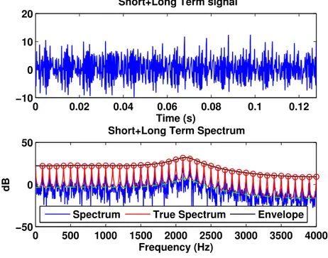
6 Spectre d’un mod`ele AR court plus long terme et du m´elange associ´e. . . . xxxvii
7 Signaux de courte dur´ee, l’observation et les sources. . . xlvi 8 Transform´ee de Fourier `a court terme, r´esultat du Alt-EMK. . . xlviii 9 L’observation, les sources et leurs estim´es obtenues avec Alt-EMK. . . xlix 10 Exemple de suppression du Vuvuzela. . . lii 1.1 Determination of the problem . . . 4
1.2 Typical NMF decomposition for audio signal. The observation is typically a Time Frequency matrix, such as the magnitude Short Time Fourier Trans-form. The decomposition finds a set of time-varying sources with constant spectrum. . . 8
2.1 A speech signal and its STFT (log magnitude). . . 19
2.2 Feedback comb filter structure. . . 20
2.3 Magnitude response for various positive values of b . . . 20
2.4 Long Term signal and its Auto correlation sequence. . . 21
2.5 Example of a periodic signal. Sampling frequency Fs = 8000Hz, b = 0.9 and τ = 0.005s. Temporal signal and its periodogram . . . 22
2.6 Example of AR signals of order p = 5. . . 24
2.7 Example of a Short plus Long term model of order p = 5. Sampling fre-quency Fs= 8000Hz, b = 0.9 and τ = 0.005s. . . 25
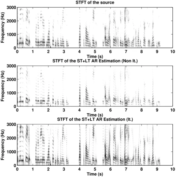
2.8 Synthesis Comparaison between iterative and non iterative methods for a real speech . . . 26
2.9 Short plus Long Term modeling of two sources and associated mixture. . . . 28
2.10 Spectra of Short plus Long Term modeling of two sources and associated mixture. . . 28
3.1 State Space Model and State Vector for 2 sources. . . 38
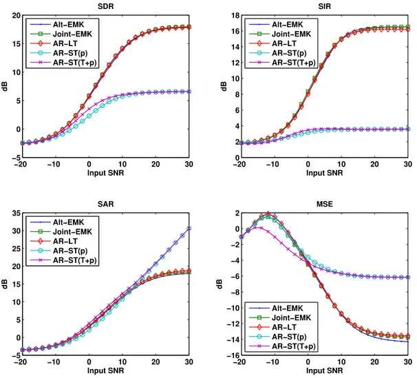
3.2 Models comparison. SDR, SIR, SAR and MSE in the filtering case. . . 44
3.3 Models comparison. SDR, SIR, SAR in the Estimation case. . . 45
3.4 With parameters estimation results, weighted sources. . . 46
3.5 Zoom on the attenuated part. . . 47
3.6 Comparison example, STFT for Joint-EMK and Alt-EMK, a fixe and a varying fondamental frequencies. . . 48
xvi LIST OF FIGURES
3.7 Comparison example, STFT for Joint-EMK and Alt-EMK, the two
fon-damental frequencies vary. . . 49
4.1 Perfect reconstruction windowing, Hann and Triangulare window with an overlap of 50% and 75%. . . 53
4.2 Comparison example Naive Versus True Minimization of IS Distance. . . 64
4.3 Example of True Minimization of IS Distance. . . 65
4.4 Perfect reconstruction windowing. . . 66
4.5 LDU Decomposition. . . 68
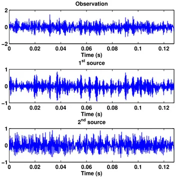
5.1 The observations and the sources, Short duration speech signals. . . 73
5.2 The sources and Estimated sources. Kalman Filter, Joint-EMK and Alt-EMK. . . 74
5.3 The sources and Estimated sources. Filtering , Naive-IS and Tmin-IS. . . 75
5.4 Models comparison. SDR, SIR, SAR and MSE in the filtering case. . . 76
5.5 Models comparison. SDR, SIR, SAR and MSE in the Estimation case. . . . 77
5.6 Models comparison. SDR, SIR, SAR and MSE in the Estimation case for different short term order. . . 77
5.7 The observation and the sources, Long duration speech signals. . . 78
5.8 STFT of sources, and estimates extracted with a Kalman filter. . . 79
5.9 STFT of sources, and estimates extracted with a Wiener filter. . . 80
5.10 Estimated Fondamental Frequency (0-500Hz) and related strenght . . . 81
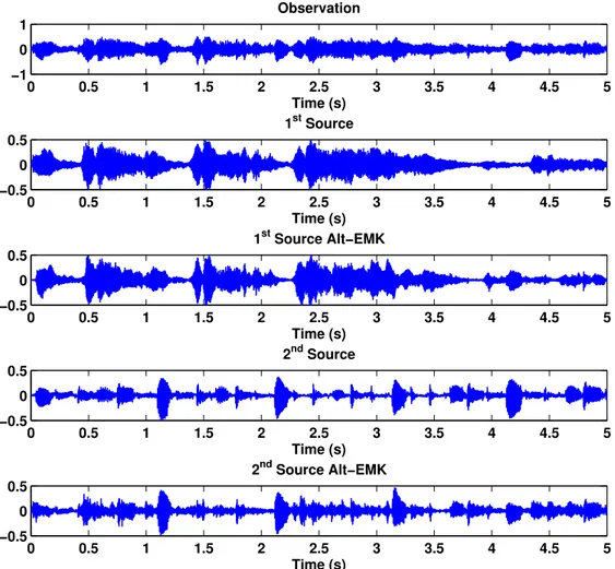
5.11 The observation, sources and estimates extracted with Alt-EMK. Long duration speech signals. . . 82
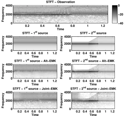
5.12 STFT of the observation, sources, and estimates extracted with Alt-EMK. 84 5.13 The observation, sources and estimates extracted with Alt-EMK. Long duration Music signals. . . 85
5.14 Vuvuzela Remover example. . . 89
A.1 Music Transcription . . . 98
A.2 A violin . . . 99
A.3 Pizzicato . . . 100
A.4 Electric Bass (5 strings) . . . 100
A.5 Slap example . . . 101
A.6 Soft (left), pratice (middle) and sustain pedals (right) . . . 101
A.7 Electro-Classical Guitar . . . 102
A.8 PalmMute . . . 102
B.1 Example of the Overlap and Add Method . . . 105
B.2 Example for the reconstruction error . . . 105
B.3 Standard deviation of the frequency error for the phase vocoder method and parabolic interpolation for a cisoid . . . 107
B.4 Estimation error of the parabolic interpolation, for one and two cisoids . . . 107
B.5 Estimation error of the parabolic interpolation and for the phase vocoder with the cleaning of the other peaks on the periodogramme . . . 107
B.6 Example of a parabolic interpolation, The circles correspond to samples of the spectrum . . . 108
B.7 General Diagram for the Harmonic+Noise Decomposition . . . 110
LIST OF FIGURES xvii B.9 Example of detection function . . . 111 B.10 Exemple of Modified Pisarenko Method on a Violin Note . . . 114 C.1 SNR Estimation for a Violin piece played by a student . . . 116
C.2 Orientation of the Bow . . . 116
C.3 Estimation of the SNR for bass sequence of two notes, the first is play with the finger and the second is play by slap. . . 117 C.4 Bass played with Finger and SNR Estimation. . . 118 C.5 Slap Bass and SNR Estimation. . . 118 C.6 Examples of waveforms of staccato, legato, staccato+ped. and legato+ped.,
note D2 . . . 120
C.7 Evolution of the amplitudes of the first three harmonics . . . 121 C.8 Harmonic+Noise Decomposition for staccato, legato, staccato+ped. and
legato+ped. . . 122 C.9 Top : Autoregressive modeling of the Noise for 170 note recordings. A
white line on top indicates notes with Pedal. Bottom : power of the AR model : For notes with Pedal (solid line) and notes without Pedal (dashed line). The dots indicate the notes that are estimated to be notes with Pedal.123 C.10 Short Time Fourier Transform, The song is composed of Non-Pizzicato and
Pizzicato notes. . . 125 C.11 Signal and onsets (a), onsets detection function and onsets (b), result of
the detection (c). . . 125 C.12 Results of the analysis for the detection of the Pizzicato for a Violin . . . . 126 C.13 STFT of notes played with and without the practice pedal . . . 126
C.14 Instantaneous frequency and amplitude tracking of a Bend, guitar note. . . 127
C.15 Instantaneous frequency and amplitude tracking of a Slide, guitar note. . . . 128 C.16 Instantaneous frequency and amplitude tracking of a Hammer, guitar note. . 128 C.17 sound containing interpretation effects, onset detection function and
instan-taneous frequency and amplitude tracking . . . 129 D.1 Illustration of the Octave Problem, Temporal point of view . . . 132
D.2 Illustration of the Octave Problem, Spectral point of view . . . 132
D.3 Difference between note and note+octave . . . 133 D.4 Even and odd parts of the spectrum. . . 135 D.5 Pitch detection and Octave Selection for a synthetic signal. . . 136 D.6 Diagram of the pitch estimation algorithm . . . 137 D.7 Octave −2 . . . 138 D.8 Octave −1 . . . 138
D.9 Good Octave . . . 139
D.10 Pitch detection and Octave Selection for guitar. . . 139 D.11 Octave problem, a note with its octave. . . 140 D.12 Octave problem in the prediction error, a note with its octave with the
temporal method (top) and the spectral method (bottom). . . 141
D.13 Octave problem in the prediction error, a note with its first and second octaves. Temporal method (top) and Spectral method (bottom). . . 142 D.14 Octave problem in the prediction error, a note with its second octave.
Tem-poral method (top) and Spectral method (bottom). . . 143 E.1 Notes on a guitar fretboard . . . 146
xviii LIST OF FIGURES E.2 Interface of the Automatic Transcription System . . . 148 E.3 Example of video errors . . . 149 E.4 Transcription Errors . . . 150 F.1 Windows and Spectra. . . 158 F.2 MultiPitch Algorithm Versus Spectral Sum. . . 162 F.3 MultiPitch Bi-Dimensional research. . . 162 F.4 Comparison Alt-EMK and Joint-EMK with non-stationary sources. . . . 163 F.5 The weight for each sources. . . 164 F.6 Estimated Noise Variance for all algorithms. . . 165
xix
Acronyms
Here are the main acronyms used in this document. The meaning of an acronym is usually indicated once, when it first occurs in the text. The English acronyms are also used for the French summary.
BSS Blind Source Separation
BASS Blind Audio Source Separation
UBSS Under-determined Blind Source Separation
LPC Linear Predictive Coding
PSD Power Spectral Densities
NMF Non-negatif Matrix Factorization
CELP Code Excited Linear Prediction
AR Auto Regressive
VQ Vector Quantization
ST Short Term
LT Long Term
SNR Signal to Noise Ration
SyNR Synthesis to Estimated Noise Ratio
MSE Mean Square Error
MMSE Minimum Mean Square Error
LMMSE Linear Minimum Mean Square Error
dB decibel
ML Maximum Likelihood
MAP Maximum A Posteriori
ADSR Attack Decay Sustain Release
KF Kalman Filter
EKF Extended Kalman Filter
SSM State Space Model
EM Expectation Maximization
RTS Rauch Tung Striebel
SAGE Space-Alternating Generalized Expectation-maximization
VB Variational Bayesian
SDR Source to Distorsion Ratio
SIR Source to Interference Ratio
SAR Source to Artefact Ratio
DFT Discret Fourier Transform
IDFT Inverse Discret Fourier Transform
xx Acronyms
LDU Lower triangular, Diagonal and Upper triangular matrix
Factor-ization
STFT Short Time Fourier Transform
MIDI Musical Instrument Digital Interface
PR Perfect Reconstruction
IS Itakura-Saito
YW Yule-Walker
SVD Singular Value Decomposition
PV Phase Vocoder
PI Parabolic Interpolation
PEA Pitch estimation algorithms
HPS Harmonic Product Spectrum
SHS Sub-Harmonic Summation
SHR Subharmonic to Harmonic Ratio
FHER Fundamental to Harmonics Energy Ratio
ESPRIT Estimation of Signal Parameters via Rotational Invariance
Tech-niques
SVM Support Vector Machine
ICA Independent Component Analysis
DUET Degenerate Unmixing Estimation Technique
CASA Computational Auditory Scene Analysis
GMM Gaussian Mixture Model
GSMM Gaussian Scaled Mixture Model
MIR Music Information Retrieval
DOA Direction-Of-Arrival
xxi
Notations
E Expectation operator
|x| Absolute value of x
⌊x⌋ Floor operation, rounds the elements of x to the nearest integers
towards minus infinity
⌈x⌉ Ceil operation, rounds the elements of x to the nearest integers
towards infinity h vector h scalar H matrix H∗ Conjugate operation HH Hermitian operation HT Transpose operation
O Matrix containing only zeros
I Identity Matrix
T Banded Toeplitz matrix
1 vector of one
diag(H) Takes the diagonal elements of a matrix
diag(h) Create a diagonal matrix with a vector
q advance operator
blockdiag block diagonal Matrix
⊕ Kronecker Sum
⊗ Kronecker Product
⊙ Hadamard Product
xxiii
Overview of the thesis and
contributions
0.1
Thesis Overview
This thesis is the results of more than four years passed at EURECOM. The original subject was: Musical Processing, that is to apply signal processing techniques on musi-cal signal and is reported in the annexe of the second part of the thesis. This work was supported by three projects namely the french ANR project: “SIEPIA”, The European Network of Excellence: “KSpace” and in parrallel the project “TAM-TAM” founded by the Institut T´el´ecom Cr´edits Incitatifs GET2007.
The project “SIEPIA” (Syst`eme Interactif d’Education et de Pratique Instrumental Acous-tique was done in collaboration with the Sart-Up SigTone [1]. The goal was to provide some tools, included in a real time simulator, for the detection of musical performances in a pedagogic context. Typically, the applications are destined to beginners musicians who want to improve their skill. The tools developped and integrated in the simulator were able to detect some defects of the bow playing for violin player, the slap playing effect for the bass guitar and the pizzicato playing for the guitar. Other tools were developped by SigTone and are not presented in this thesis, they include real time chords recognition, real time automatic guitare transcription and comparison (with a predefined piece), tempo analysis etc. This simulator was presented during the “Grand Colloque STIC 2006 ” (with a high background noise) in Lyon (France), and was ranked in the first eight best projects of the competition (over more than 140 projects). Unfortunately the collaboration has stopped with the project.
Our contributions in the project “KSpace” (Knowledge Space of semantic inference for automatic annotation and retrieval of multimedia content) was more fuzzy. The aim of the research was to narrow the gap between low-level content descriptions and subjectivity of semantics in high-level human interpretations of audiovisual media. For this project we have continued to provide low level tools related to the detection of musical interpretation effects for the guitar and the piano. We also propose a solution for solving the octave probeme which appears when a note and its octave are played together. Then during a “KSpace” PhD workshop, in the last year of the project, an idea of collaboration with the EURECOM Multimedia Department born. The work of Marco Paleari was focused on emotional analysis of facial gesture [2] and gave us, at the begining, the idea of analysing facial gesture of musician (as a violinist performing a solo sequence) in order to evaluate the degree of emotion. As this analysis was highly specialized and, also, as a very special-ized database was needed, we gave up the idea. However, we change it. The new concept
xxiv Overview of the thesis and contributions was to make an audio-visual analysis of a guitar player for solving some ambiguities that are difficult to solve with only the Audio part. In parrallel we discover the work of Olivier Gillet [3] which a part focused on the audio-visual analysis of drum song. This work was an intra department collaboration in EURECOM and allowed us to supervize students projects leading to a prototype of the simulator.
The “TAM-TAM” Project (Transcription automatique de la musique : Traitements avanc´es et mise en oeuvre) was done with the TSI departement of T´el´ecom Paris Tech and in parrallel with the “KSpace” Project. The goal of this project was the Automatic Transcription of piano songs. Our contributions was to provide an analysis of the MIDI protocol, not presented in this thesis, for the trancription (advantage and drawback). Also we propose to work on the detection of the Sustain Pedal of the piano. We propose a method which was able to detects the presence of the pedal on our database and for single note. However, normally the pedal is used for playing a succession of notes which are normally infeasible. So the single note case is not interesting but if the conditions allow the detection of the pedal, the analysis was able to find something that the ear is not abble to detect.
When these projects were finished and due to the lack of consistent database we stopped to work on Musical Processing. However all this works were considered as original at least in terms of issues addressed.
The first part of the thesis is related to one another project collaboration between the TSI departement of T´el´ecom Paris Tech, the Multimedia and Mobile Department of EURE-COM: The Institut Telecom “Futur et Ruptures” project “SELIA” (Suivi et s´eparation de Locuteurs pour l’Indexation Audio. The aim of the project was to focuse on audio document indexing by investigating new approaches to source separation, dereverberation and speaker diarization. Our task in this project was to propose new Mono-Microphone Source Separation Algorithms. This project give us the opportunitie to supervize a Mas-ter project in the person of Siouar Bensaid who is now a PhD Student at EURECOM. Together we work on an Adaptive EM-Kalman Algorithm and she continue to work on it while I begin to analyse Frame Based Algorithm.
0.2. CONTRIBUTIONS xxv
0.2
Contributions
These contributions are divided into two parts:
• Mono-Microphone Blind Audio Source Separation • Musical Processing.
A brief overview of the general framework of this thesis, and of each part is given in this section.
0.2.1 Blind Audio Source Separation
The first part deals with Mono-Microphone Blind Audio Source Separation (BASS). This is considered as a difficult problem because only one observation is available. In fact it is the most under-determined case, but also the more realistic one for many applications. A vast number of fast and effective methods exist for solving the determined problem [4, 5]. In the under-determined case, the number of sources n is greater than the number of mix-tures m and the problem is degenerate [6] because traditional matrix inversion (demixing) cannot be applied. In this case, the separation of the under-determined mixtures requires prior [7, 8] information of the sources to allow for their reconstruction. Estimating the mixing system is not sufficient for reconstructing the sources, since for m < n, the mixing matrix is not invertible. Here we focus on the presumed quasi periodic nature of the sources.
Chapter 1
The first Chapter is an introductive chapter. The goal of this chapter is to motivate the BSS problem and to recall some existing solution. We recall some general definitions of the Source Separation Problem as well as a summary of a majority of the possible cases. More specially we focus on the Mono-Microphone literrature. We motivate the model and the approach that we will use.
Chapter 2
Chapter 2 is dedicated to the description of the source model. Here we model speech as a combination of a sound source: the vocal cords and a linear acoustic filter [9]. We assume that a source can be represented by the combination of auto-regressive (AR) mod-els; the periodicity is represented by a long term AR model followed by a short term AR for its timbre. This model is largely used in CELP codding but it didn’t receive a lot of interest in the BASS community, despite of its simplicity. In this chapter we explain the parametric model of a source and of the mixture. For each AR models of a source the correlation lenghts are very different and are related to different parameters.
Chapter 3
The first algorithm that we have designed is an adaptive Expectation Maximization (EM) Kalman Filtering (KF) algorithm. The KF corresponds to optimal Bayesian estimation of the state sequence if all random sources involved are Gaussian. The EM-Kalman algo-rithm permits to estimate parameters and sources adaptively by alternating two steps :
xxvi Overview of the thesis and contributions E-step and M-step [10]. As we focus on speakers’ separation, an adaptive algorithm seems to be ideal for tracking the quick variations of the considered sources. The traditional smoothing step, needed for the M-Step, is included in the state space model. Chapter 3 presents the algorithm and associated results which have been presented in:
• S. Bensaid, A. Schutz, and D. T. M. Slock, Monomicrophone blind audio source separation using EM-Kalman filters and short+long term AR modeling, 43rd Asilo-mar Conference on Signals Systems and Computers, November 1-4, 2009, AsiloAsilo-mar, California, USA.
• S. Bensaid, A. Schutz, and D. T. M. Slock, Single Microphone Blind Audio Source Separation Using EM-Kalman Filter and Short+Long Term AR Modeling, in LVA-ICA, 9th International Conference on Latent Variable Analysis and Signal Separa-tion, September 27-30, 2010, St. Malo, France.
Chapter 4
We consider the problem of parameters estimation as well as the source separation in a frame based context. We present, in particular, two algorithms based on the Itakura-Saito (IS) Distance for estimating the parameters of the sources individually. The estimation is done directly from the mixture and without alternating between the separation of the sources and the estimation of the parameters. The first algorithm is derived from a naive interpretation of the IS distance. It consists on alternatively estimating the short term and long term subsets of parameters. Each subset estimation needs to be iterated between all the sources (including the additive noise) until convergence. The second one is based on the true minimization of the IS distance but it is still unfinished. We remark in partic-ular that the IS gradient is the same as for Optimally Weighted Spectrum Matching and Gaussian ML.
• Antony Schutz and Dirk T M Slock, ”Blind audio source separation using short+long term AR source models and iterative itakura-saito distance minimization,” in IWAENC 2010, International Workshop on Acoustic Echo and Noise Control, August 30-September 2nd, Tel Aviv, Israel.
• Antony Schutz and Dirk T M Slock, ”Blind audio source separation using short+long term AR source models and Spectrum Matching”, accepted in DSPE 2011, Inter-national Workshop on Digital Signal Processing and Signal Processing Education, January 4-7, Sedona Arizona, USA.
Then we focus on a frame based source separation algorithm in a Variational Bayesian context. The separation is done in the spectral domain. In the formulation of the problem, the convolution operation is done by a circulant matrix (circular convolution). We have introduced a more rigorous use of frequency domain processing via the introduction of carefully designed windows. The design of the window and the use of circulant matrices lead to simplication. The frame based algorithm extracts the windowed sources and is non-iterative. This work was presented in:
• A. Schutz and D. T. M. Slock, Single-microphone blind audio source separation via Gaussian Short+Long Term AR Models, in ISCCSP 2010, 4th International Sym-posium on Communications, Control and Signal Processing, March 3-5, Limassol, Cyprus.
0.2. CONTRIBUTIONS xxvii Chapter 5 and 6
The Chapter 5 is dedicated to simulations on real signals. We have used speech (a man and a woman) and instrumental (cello and guitare) mixture on long duration. In the considered mixture the signal are non stationary, everything move. Sometimes the sources are not active, theirs periods varies. We compare the proposed algorithm, and mainly the so called Alt-EMK in a source separation context. We have also used this algorithm for the background extraction task involving data from the FIFA world cup 2010 in or-der to remove the vuvuzellas from the original signals. In Chapter 6 we give the general conclusion of our work and some possible improvement to take into account.
0.2.2 Annexe: Musical Processing
The second part of the thesis is about Musical Processing which is a very general topic. We mean by Musical Processing that all the work is related to music and more precisely to musical instruments. Several tools were developed and presented; some of which were implemented in a real time simulator and have given the expected results. Most of the work focus on the detection of interpretation effects. We present a work about the detection of the octave when it is played with a note and the last Annexe deals with an Audio-Video simulator for the analysis of a guitar player.
In this part we don’t use the same model as in the first part, we use the sinusoidal plus noise model [11]. A sound is described as a sum of a sinusoid plus an additive noise. The frequencies, the amplitudes and the phases of the sinusoids are unconstrained.
Annexe A describes the musical instruments, the interpretation effects and the playing defects that will be analysed after. The instruments considered here are the Guitar, Bass, Violin, Piano.
Annexe B describes all the tools developed for the detection and Annexe C the asso-ciated results. We present an analysis/synthesis algorithm for obtaining the deterministic and the stochastic parts of the model, where the model is composed of harmonic (deter-ministic) and residual (stochastic part). The obtained residual component is composed of the noise, the roundoff/approximation errors and what we call the instrumental noise. The instrumental noise is a kind of signature, for a violin it is mainly due to the bow, for a piano it is more linked to the soundboards and to the hammers etc. This Harmonic plus Noise decomposition is also a transient detector when the separation is correctly per-formed. For example, if a violin is played by a good musician the resulting sound will be better (stronger harmonic part) and more constant than by a beginners’. The defects of the beginner are also hidden in his bowing techniques, the pressure, the orientation and the constancy of the displacement are important, and a defect on one of these points leads to noise apparition in the resulting note. Several interpretation effects are investigated for the guitar but no particular features are detected except that, in the most general case, an interpretation effect can be summarized as a frequency variation with only one attack. • A. Schutz and D. T. M. Slock, ”Mod´ele sinuso¨ıdale: Estimation de la qualit´e de jeu dun musicien, d´etection de certains effets d’interpr´etation,” in GRETSI 2007, 21eme colloque traitement du signal et des images, September 11-14, 2007, Troyes, France. • A. Schutz and D. T. M. Slock, ”Estimation of the parameters of sinusoidal signal components and of associated perceptual musical interpretation effects,” in Jamboree
xxviii Overview of the thesis and contributions 2007: Workshop By and For KSpace PhD Students, September, 14th 2007, Berlin, Germany.
• A. Schutz and D. T. M. Slock, ”Toward the detection of interpretation effects and playing defects,” in DSP 2009, 16th International Conference on Digital Signal Pro-cessing, July 05-07, 2009, Santorini, Greece.
• A. Schutz, N. Bertin, D. Slock, B. David, and R. Badeau, ”Piano forte pedal analysis and detection,” AES124, 2008.
In Annexe D we present an analysis of the octave problem. The octave problem appears when a note and its octave are present together. As the octave has a frequency twice as the note. If we don’t take the inharmonicity into consideration, then they share the same periodicity and the partials of the spectrum are perfectly overlapped which makes the detection difficult. We propose, in this Annexe, an energetic criteria based on the energy of the odd and even partials of the chord. But we are not working in the spectral domain. We show that the odd and even harmonics of the spectrum can be represented by the odd and the even parts of a cyclic correlation. This method is also used as a pitch detector, the set of fundamental frequency has to be defined. It works in two steps; first the pitch is found in the lower octave of the instrument and then the good octave of the note is found. This approach assumes that the signal is harmonic and fails if it is not.
• A. Schutz and D. T. M. Slock, ”Periodic signal modeling for the octave problem in music transcription,” in DSP 2009, 16th International Conference on Digital Signal Processing, July 05-07, 2009, Santorini, Greece.
Annexe E gives the description of an audio-video simulator specialized for guitar. A guitar can indeed chime the same note (i.e. a note with the same pitch) at different positions of the fretboard on different strings. This is why the musical transcription of a guitar usually takes form of a tablature. A tablature is a musical notation which includes six lines (one for each guitar string) and numbers representing the position at which the string has to be pressed to perform a note with a given pitch. The proposed approach combines information from video (webcam quality) and audio analysis in order to provide the tablature. We have investigated the monophonic case, one note at a time. The audio processing is composed of an onset detector followed by a mono-pitch estimation algorithm. In case of a tablature the duration of the note is not needed. The first frame of the video is analyzed to detect the guitar and its position, then we make use of the Tomasi Lukas Kanade algorithm to follow the same points, corresponding to each string/fret intersection along the video. Filtering is done on the frame to detect the skin color and to estimate the hand position. Then knowing the pitch and the position of the hand we estimate the string and the fret which was played.
• M. Paleari, B. Huet, A. Schutz, and D. T. M. Slock, ”A multimodal approach to music transcription,” in 1st ICIP Workshop on Multimedia Information Retrieval : New Trends and Challenges, October 12-15, 2008, San Diego, USA.
• M. Paleari, B. Huet, A. Schutz, and D. T. M. Slock, ”Audio-visual guitar transcrip-tion,” in Jamboree 2008, Workshop By and For KSpace PhD Students, July, 25 2008, Paris, France.
xxix
R´
esum´
e des travaux de th`
ese
Ce chapitre est un r´esum´e r´edig´e en Fran¸cais du pr´esent document. Il reprend les grands axes du document originellement ´ecrit en Anglais. Dans une premi`ere partie, nous intro-duisons le probl`eme de la s´eparation aveugle de source puis le cas monomicrophone ainsi que le positionnement du travail. Nous exposons ensuite le mod`ele de production de la parole utilis´e dans cette th`ese. Nous proposerons deux types d’algorithme, les premiers sont adaptatifs et les suivants sont bas´es sur une analyse par fenˆetre. Les syst`emes mis en oeuvre sont alors d´ecrits. Enfn nous concluons ce chapitre par un r´esum´e de nos
contribu-tions et d´eveloppons certaines pistes `a explorer `a l’avenir pour am´eliorer les performances
des syst`emes pr´esent´es.
0.3
Introduction `
a la s´
eparation aveugle de source
La s´eparation aveugle de source (SAS) est une discipline g´en´erique qui consiste `a estimer K
sources `a partir de N observations. Elle trouve place dans de nombreuses disciplines tel que:
le traitement audio, le traitement d’image, les t´el´ecommunications, le g´enie biom´edical etc. [12]. Suivant le type d’application envisag´e la nature des sources et des capteurs varient, dans le cas de l’audio les sources seront soit des instruments de musique soit de la parole et les capteurs seront des microphones. Les sources, les quantit´es qui nous int´eressent, sont
inconnues ainsi que le processus li´e `a leur propagation jusqu’aux microphones. Chaque
microphone captera une observation, diff´erente, qui sera un m´elange d´eform´e des sources d’origine. Les applications concern´ees sont par exemple dans le traitement audio: analyser les sources ind´ependamment et de mani`ere automatique pour des applications de parole vers texte [13], r´ehaussement de la parole [14], reconnaissance de locuteur. Si l’on consid`ere
des applications li´ees `a la musique tel que la reconnaissance automatique d’instrument [15]
ou la transcription automatique de la musique [16, 17], analyser une source `a la fois aidera
grandement le proc´ed´e. La SAS s’applique ´egalement aux applications d’extraction de la m´elodie principale [18] la restauration d’enregistrement ancien [19, 20], suppression de la
voi pour le karaoke [18, 20], l’aide `a l’´ecoute [12, 21] etc. La SAS trouve cependant de
nombreuses formulations en fonction du type de probl`eme rencontr´e, la Figure 1 permet de r´esumer ces diff´erents cas auxquels ont peut ˆetre confront´e:
• Le cas sous d´etermin´e extrˆeme, si seulement une observation est pr´esente. • Le cas sous d´etermin´e, quand il y a moins de capteurs que de sources. • Le cas d´etermin´e, quand on a autant de sources que de capteurs.
xxx R´esum´e des travaux de th`ese
Figure 1: D´etermination
La propagation des sources jusqu’aux capteurs tient aussi un rˆole essentiel dans la d´efinition
du probl`eme. On peut diff´erencier plusieurs cas:
• Les m´elanges lin´eaires instantan´es sont les plus simples. Dans ce cas chaque observa-tion est la somme pond´er´ee des sources. Si on ´ecrit les coefficients de m´elanges dans
une seule matrice (appel´e la matrice de m´elange) le probl`eme se r´esume `a identifier
cette matrice et `a l’inverser.
• Les m´elanges att´enu´es et d´ecal´es sont rencontr´es lorsque les observations sont com-pos´ees de versions att´enu´ees et temporellement d´ecal´ees des sources. Une source n’arrive pas au mˆeme moment sur tous les capteurs, pour chaque sources et pour chaque capteur ce d´ecalage est diff´erent.
• Les m´elanges convolutifs sont eux les plus g´en´eraux. Dans ce cas chaque sources est filtr´ee avant l’acquisition par un capteur.
• Les m´elanges non lin´eaires n’ont ´et´e ´etudi´es que dans des cas particuliers, comme lorsque la non lin´earit´e est introduite au moment de l’acquisition (Post non lin´eaire)
0.3.1 Quelques solutions existante
La SAS est apparue au milieu des ann´ees 1980 et `a ´et´e tout d’abord formul´ee par H´erault,
Ans et Jutten [22–24] pour les m´elanges lin´eaires instantan´es [23] puis, dans les ann´ees 90 pour le cas convolutif [25, 26]. Comon a introduit l’analyse en composantes ind´ependentes (ACI) en 1991 [27, 28], bien que de nombreux travaux aient ´et´e ´elabor´es avant, la plu-part d’entre eux peuvent ˆetre inclus dans l’ACI. L’id´ee original de l’ACI envisage le cas
d´etermin´e de m´elange instantan´e et cherche `a trouver l’inverse de la matrice de m´elange
qui rend les sources les plus ind´ependantes possible. Si l’on peut consid´erer les sources ind´ependantes, au sens statistique du terme, il est plus difficile de consid´erer que les
observations le soient aussi. Une variante de l’ACI consiste `a minimiser l’information
mutuelle qui est aussi une mesure d’ind´ependance entre des variables al´eatoires [29]. Suiv-ant le mˆeme ´etat d’esprit, si un signal se retrouve parcimonieux dans une certaine base
0.3. INTRODUCTION `A LA S ´EPARATION AVEUGLE DE SOURCE xxxi ou transformation alors la somme des signaux le sera moins, de ceci resultera la recherche
de solution amenant `a maximiser la parcimonie des sources [30]. Les m´ethodes bas´ees
sur l’utilisation de dictionnaires cherche donc `a estimer les coefficients li´es aux
dictio-nnaire et non les s´erie temporelle elle mˆeme [30, 31]. Les s´eries seront reconstruites `a
partir du dictionnaire et des coefficients estim´e, l’id´ee est de d´ecomposer les
observa-tions (Y ) `a partir d’un dictionnaire connu(φ), en prenant en compte qu’il y a une
ma-trice de m´elange (A) et une mama-trice de coefficients (C) ce qui am`ene au syst`eme suivant Y = ACφ il faudra donc trouver les deux matrices A et C tel que C soit le plus parci-monieux. possible. Dans le cas sous d´etermin´e, trouver la matrice n’est pas toujours faisable et dans ce cas son inversion n’est pas possible. Cependant ce cas, qui est plus r´ealiste que les cas (sur)d´etermin´e apparaˆıt fr´equemment. Pour pouvoir s´eparer il faut avoir une information a priori sur les sources [7, 8] comme une hypoth`ese de parcimonie dans une certaine base. Par exemple l’algorithme DUET [32, 33] consid`ere que les sources
sont d´ej`a s´epar´ees dans le plan temps fr´equence, ce que les auteurs appellent la propri´et´e
d’orthogonalit´e W-Disjoint, et qu’un masque binaire peut ˆetre appliqu´e pour la s´eparation. Le cas sousd´etermin´e inclus le cas st´er´eophonique, le dernier cas avant le cas sous-determin´e extrˆeme. Le fait d’avoir deux observations est le cas limite pour utiliser des informations spatiales et une campage d’´evaluation lui est d´evolue [34, 35]. Pour des enregistrements st´er´eophoniques, [36, 37] prennent l’hypoth`ese qu’une source est dominante dans un des deux canaux, g´en´eralement les caract´eristiques ´etudi´ees sont les diff´erences de puissance et/ou de phase entre les canaux et permettent de remonter jusqu’aux angles d’arriv´ee des sources, avec une telle information on peut alors former un masque temps fr´equence et s´eparer les sources [6, 33, 38–41]. Cependant si les sources sont trop proches les unes des autres ou que d’une mani`ere g´en´erale ces caract´eristiques sont trop similaires les methodes failliront.
0.3.2 Positionnement du travail expos´e
Dans le travail expos´e dans cette th`ese nous nous placerons dans le cas Mono-Microphone, nous consid´ererons aussi bien le cas des m´elanges lin´eaires instatann´ees que les cas att´enu´es et d´ecal´es. Puisque nous ne pouvons, avec un seul microphone estimer les possibles retards
et att´enuations des signaux. Bien que les algorithmes ne soient pas restreints `a ce cas
pr´ecis, nous utiliserons dans les simulations des observations compos´ees de deux sources plus un bruit blanc. Nous envisageons aussi bien des signaux de parole que de musique.
0.3.3 La s´eparation aveugle de source Mono-Microphone
Le cas mono-microphone est qualifi´e de sous-d´etermin´e extrˆeme et est sans doute le plus difficile puisque dans ce cas pr´ecis aucune information spatialle ne peut ˆetre utilis´ee. Nous sommes oblig´es de mod`eliser les sources afin de contraindre la solution. Il est n´eanmoins, pour beaucoup d’applications le plus r´ealiste, si l’on consid`ere que y(t) est une observation
compos´ee par exemple de deux sources x1(t) et x2(t) tel que y(t) = x1(t) + x2(t) et bien
n’importe quelle solution s(t) satisfaisant ˆx1(t) = s(t) et ˆx2(t) = y(t) − s(t) sera une
solu-tion ´evidente du probl`eme [42]. Cet exemple met en exergue la n´ecessit´e de mod´eliser les sources afin de contraindre les solutions. Pour cela il a ´et´e propos´e d’utiliser diff´erents types de mod´elisation, les premi`eres utilisent des mod`eles dont les param`etres sont issues d’un certain apprentissage, les suivantes ont pour but de s’adapter (dans une certaine mesure) aux donn´ees. Dans la premi`ere cat´egorie, parmi les approches utilis´ees citons la
xxxii R´esum´e des travaux de th`ese
La premi`ere ´etape consiste `a apprendre des vecteurs sur des donn´ees d’entrainement puis
`
a trouver la meilleure combinaison de ces vecteurs pour repr´esenter la source. Dans cet esprit [43], Roweis utilise une repr´esentation log magnitude d’une transform´ee de Fourier `
a court terme associ´e `a l’approximation Log-Max log( a + b ) ≈ max ( log(a), log(b) )
ainsi chaques points temps fr´equence n’appartient qu’`a une source. Puis viennent les mod`ele de m´elanges de Gaussienne (MMG), l’id´ee est de repr´esenter chaque source par la r´ealisation d’une variable al´eatoire repr´esent´ee par un ensemble fini de formes spectrales caract´eristiques. Dans [44], un probl`eme consid´erant deux sources est analys´e, chaque
source est mod`elis´ee `a partir de Q ´etats et chaque ´etat q est repr´esent´e par une enveloppe
spectrale et une distribution a priori, la s´eparation est effectu´e par l’utilisation d’un filtre de Wiener ”adaptatif”. Comme plusieurs trames temporelles cons´ecutives poss`edent plus
ou moins le mˆeme contenu, c’est `a dire un mˆeme spectre dont seul l’intensit´e varie, les
au-teurs introduisent le mod`ele de m´elange de Gaussiennes amplifi´ees (MMGA), qui permet
de dinstinguer l’intensit´e de la forme spectrale [45]. Dans le cas o`u les donn´ees apprises
ne collent pas tr`es bien aux donn´ees observ´ees une adaptation du mod`ele est envisag´ee dans [42]. L’´evolution temporelle des param`etres peut ˆetre pris en compte en remplacant le mod`ele de m´elange de Gaussienne par un mod`ele de Markov cach´e (MMC). Les MMC peuvent ˆetre vue comme une g´en´eralisation des MMG. Roweiss [46] discutte l’utilisation de MMC factoriel, dans son approche les MMC/MMG sont appris pour chaque source
sur des sons isol´es puis appliqu´es `a un m´elange, la s´eparation utilise un masque binaire
dans le plan temps fr´equence dans lequel les sources sont suppos´ees disjointes. Benaroya et al. [44] utilisent aussi des MMC, leur conclusion est que l’am´elioration apport´ee par les MMC compar´es au MMG n’est pas significative, au vue de certains crit`eres d’´evaluations. La s´eparation et l’analyse s’op`ere d’une mani`ere g´en´erale dans le plan temps fr´equence. Il en r´esulte en l’analyse d’une matrice (temps et fr´equence) dont les ´el´ements sont posi-tifs. La factorisation en matrice non n´egative (FMN) devient donc un outil logique pour l’analyse. Le concept est de s´eparer une matrice non n´egative en deux matrices non n´egatives, la d´efinition de ces deux matrices d´epend de l’application vis´ee et est illustr´e
dans le cas de l’audio dans le Figure 2. La FMN est devenue tr`es propulaire grace `a
l’apparition d’algorithme rapide invoquant des mises a jours multiplicatives.
Originelle-ment attribu´ee `a Lee et Seung [47], ces mise `a jour sont connues depuis longtemps dans
le traitement d’image, notamment la d´econvolution d’image [48] dans le cas o`u la matrice
de base est connue [49] ou partiellement [50, 51] voir estim´ee. Les deux matrices sont appel´ees dans le cas de l’audio la matrice de base, contenant des spectres caract´eristiques (spectre repr´esent´e par des peignes de fr´equences fondamentales diff´erentes) et une matrice d’activation, qui elle, est estim´ee. Si le spectre d’une certaine colonne est pr´esent dans le
signal alors la ligne de la matrice d’activation correspondante `a cette colonne sera activ´ee,
d´ecrivant l’´evolution de l’intensit´e du spectre consid´er´e.
0.3. INTRODUCTION `A LA S ´EPARATION AVEUGLE DE SOURCE xxxiii Parmis les m´ethode utilisant des mod`eles s’adaptant aux donn´ees le plus connu est le
mod`ele sinusoidale bruit´e [11, 52]. Dans ce cas l`a un son est une somme de sinusoides
har-moniques, inharhar-moniques, le but consiste `a d´etecter dans le spectre les pics correspondant
`
a une note (d’o`u la contrainte d’harmonicit´e) puis d’estimer leurs amplitudes et phases
afin de reconstruire la note seule. Plusieurs probl`emes sont rencontr´es comme la pr´ecision qui peut ˆetre am´elior´ee en utilisant des interpolations sur les maximas locaux [53–55], le recouvrement fr´equentiel qui peut ˆetre pali´e en utilisant une contrainte sur l’enveloppe
spectrale r´esultante la for¸cant `a ˆetre douce [56]. D’autres travaux utilisent la m´ethode de
”matching pursuit” (MP) qui consiste `a d´ecomposer un signal en atome ´el´ementaire [57].
Leveau dans [15] propose d’utiliser des atomes li´es `a chaque note de plusieurs
instru-ments rendant l’estimation des notes et de l’instrument conjointe. Triki [58] consid`ere l’extraction de signaux p´eriodiques avec une faible modulation d’amplitude et de phase et rend compte que dans les zones les plus harmoniques sa m´ethode donne de meilleur r´esultat alors que le MP [57] est meilleur pour les zones transitoire (fortement non sta-tionnaire). Un autre type de mod´elisation est la mod´elisation autor´egressive (AR) ainsi certains auteurs utilisent des filtres en peigne [59], qui peuvent ˆetre impl´ement´es en util-isant des p´eriodes non enti`eres [60]. Emiya [17] mod`elise une note comme un processus
AR pour la note et `a moyenne mouvante (MM) pour le bruit (les vall´ees entre les pics),
en utilisant un crit`ere de maximum de vraisemblance il est capable de s´eparer des pi`eces polyphoniques. [61] Carpentier et al. utilise un filtre Kalman avec une mod´elisation AR de
faible ordre et montre que les sources peuvent ˆetre s´epar´ees `a condition que les supports
soient diff´erents.
Nous consid´ererons un m´elange de ces derniers mod`eles, une source sera repr´esent´ee par
sa p´eriodicit´e grˆace `a un filtre en peigne alors que les enveloppes spectrales, elles, seront
mod´elis´ees par un filtre AR d’ordre faible. Ce mod`ele qualifi´e de mod`ele source filtre est tr`es proche de celui utilis´e par Durrieu [18]. Son mod`ele utilise une partie connue, un dictionnaire de fr´equence fondamentale utilis´e de la mˆeme mani`ere que les FMN. Nous ne contraignons pas notre mod`ele.
Pour plus d’information
L’´etat de l’art pr´esent´e dans cette partie peut ˆetre compl´et´e par une lecteur des documents suivants
• La factorisation de quantification vectorielle, une analyse peut ˆetre trouv´ee dans la th`ese de Ron J. Weiss [62].
• Pour le mod`ele de m´elange de Gaussien (Amplifi´e ou pas), le mod`ele de Markov cach´e ainsi que le Filtre de Wiener Adaptatif, nous nous r´efererons aux th`ese de Laurent Benaroya [63], Alexey Ozerov [64] et Jean-Louis Durrieu [18].
• La factorisation en matrice non n´egative appliqu´ee `a la transcription automatique de la musique, la th`ese de Nancy Bertin y est consacr´ee [16].
• La s´eparation bas´ee sur le mod`ele sinusoidale bruit´e peut ˆetre trouv´ee dans la th`ese
de Tuomas Virtanen [65] et dans la th`ese de Mahdi Triki [66] o`u l’on trouve aussi
une revue des approches de type MP.
• La mod´elisation ARMM pour la transcription de la musique dans la th`ese de Valentin Emiya [17].
xxxiv R´esum´e des travaux de th`ese
0.4
Mod`
ele utilis´
e
Comme indiqu´e dans la section pr´ec´edente nous utiliserons un mod`ele param`etrique. Ce mod`ele est tr`es proche du mod`ele CELP utilis´e dans le codage de la parole. Il s’agit d’un modle source-filtre qui prend en compte les deux aspects principaux d’un son: l’aspect p´eriodique et le timbre.
0.4.1 La parole
Une base th´eorique largement utilis´ee pour la mod`elisation de la parole est le mod`ele source filtre. Ce mod`ele est bas´e sur la combinaison de deux aspects: les cordes vocales et un filtre acoustique lin´eaire [9]. Bien que ce mod`ele ne soit qu’une approximation, il a ´et´e
largement utilis´e et ceci, essentiellement, grˆace `a sa robustesse et sa simplicit´e. Ce mod`ele
est bas´e sur l’hypoth`ese que la parole peut ˆetre mod`elis´ee par l’utilisation de deux aspects ind´ependents l’un de l’autre. Ainsi les vibrations engendr´ees par les cordes vocales et les r´esonnateurs n’ont aucune interaction. Au point de vue impl´ementation, la technique la plus utilis´ee reste la mod`elisation tout-pˆole ou la pr´ediction lin´eaire [67]. De cette mani`ere la, l’excitation est mod´elis´ee par un train d’impulsion qui est filtr´ee par le filtre tout-pˆole.
0.4.2 Mod´elisation `a long terme
Comme indiqu´e pr´ec´edement, la mod´elisation `a long terme s’effectuera par l’interm´ediaire
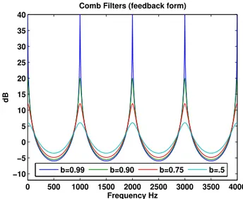
d’un train d’impulsion qui entraˆıne, dans le domaine fr´equentiel, un peigne fr´equentiel. Une mani`ere de g´en´erer ce peigne est l’utilisation de filtre en peigne dont la r´eponse en magnitude est donn´ee dans la Figure 4.
Figure 3: Filtre en peigne en mode ”Feedback”.
0 500 1000 1500 2000 2500 3000 3500 4000 −10 −5 0 5 10 15 20 25 30 35 40 Frequency Hz dB
Comb Filters (feedback form)
b=0.99 b=0.90 b=0.75 b=.5