Évaluation du potentiel de croissance des arbres feuillus et de leur sensibilité aux conditions climatiques

(1)

Évaluation du potentiel de croissance des arbres

feuillus et de leur sensibilité aux conditions climatiques

Thèse

Guillaume Moreau

Doctorat en sciences forestières

Philosophiæ doctor (Ph. D.)

(2)

Évaluation du potentiel de croissance des

arbres feuillus et de leur sensibilité aux

conditions climatiques

Thèse

Guillaume Moreau

Sous la direction de :

David Pothier

Alexis Achim

(3)

Résumé

En Amérique du Nord, la coupe de jardinage a été implantée en réponse à plusieurs décennies de mauvaises pratiques forestières ayant laissé de grandes superficies de peuplements feuillus dégradés et de faible vigueur. Or, l’application de la coupe de jardinage dans un contexte industriel a produit des résultats variés et parfois peu convaincants sur sa capacité à améliorer la vigueur générale des peuplements et à fournir un rendement soutenu en bois de haute valeur. L’objectif général de ce projet de recherche était d’améliorer les prévisions de la croissance et de la mortalité des arbres feuillus à partir d’une meilleure évaluation de leur potentiel de croissance sur pied et de leur sensibilité aux conditions climatiques. Nos résultats ont d’abord montré un effet marginal du taux de dégagement induit par la coupe de jardinage sur la croissance et le taux de survie des arbres résiduels. Ce résultat s’explique en partie par une concentration de la récolte des arbres à l’intérieur et aux abords des sentiers de débardage, laissant ainsi de larges zones non traitées dans les peuplements résiduels. Dans les années suivant l’application du traitement, uniquement 24 % des arbres ont connu une hausse de croissance significative, un pourcentage de réaction de croissance légèrement inférieur à celui induit par les perturbations naturelles au cours des décennies précédentes. Nos analyses ont également montré qu’une réduction marquée de la croissance sur plusieurs décennies précédait 88 % des événements de mortalité post-récolte, et que les prévisions de ces événements pouvaient être significativement améliorées en considérant les tendances de croissance 25 ans avant la coupe. De plus, la présence de défauts affectant la vigueur des arbres au moment de la coupe était positivement reliée à la probabilité de mortalité et négativement reliée à la probabilité d’avoir une hausse de croissance après la coupe. Par ailleurs, nos analyses ont montré qu’une évaluation visuelle de la densité du houppier est l’indicateur le plus efficace pour estimer la vigueur et le potentiel de croissance sur pied de l’érable à sucre. Finalement, nos analyses des relations entre la croissance et les conditions climatiques ont montré un lien fort entre l’occurrence des stress climatiques ponctuels et une diminution de la croissance de l’érable à sucre. Les épisodes de gel-dégel de forte intensité ont été particulièrement dommageables en provoquant des baisses abruptes de la croissance dans les deux régions étudiées. À l’inverse, les analyses provenant des tendances climatiques mensuelles ont indiqué une relation faible et instable dans le temps avec la croissance. Nos résultats indiquent que l’effet synergique d’une accumulation de plusieurs stress climatiques et d’épidémies d’insectes défoliateurs au début des années 1980 a induit un changement

(4)

important dans la dynamique de croissance de l’érable à sucre et sa réponse aux conditions climatiques mensuelles.

(5)

Table des matières

Résumé ... ii

Table des matières ... iv

Liste des figures ... viii

Liste des tableaux ... ix

Remerciements ... x

Avant-propos ... xii

Insertion d’articles ... xii

Coauteurs des chapitres ... xiii

Introduction ... 1

Démarche méthodologique ... 6

1. Chapitre 1 Growth and survival dynamics of partially cut northern hardwood stands as affected by precut competition and spatial distribution of residual trees ... 8

1.1. Abstract ... 9

1.2. Résumé ... 10

1.3. Introduction ... 11

1.4. Material and methods ... 13

1.4.1. Sampling sites ... 13

1.4.2. Sample plots and treatments ... 13

1.4.3. Data collection ... 15

1.4.4. Competition index ... 16

1.4.5. Modelling harvest probability ... 17

1.4.6. Modelling the radial growth response ... 17

1.4.7. Modelling survival probability ... 18

1.4.8. Model selection ... 18

1.5. Results ... 19

1.5.1. Harvest probability ... 19

1.5.2. Growth response ... 21

1.5.3. Post-cut survival model ... 22

1.6. Discussion ... 24

1.6.1. Post-cut tree spatial pattern and growth response ... 24

1.6.2. Post-cut survival ... 26

(6)

1.6.4. Silvicultural implications ... 28

1.7. Conclusion ... 29

1.8. Acknowledgements ... 30

1.9. References ... 31

2. Chapitre 2 A dendrochronological reconstruction of sugar maple growth and mortality dynamics in partially cut northern hardwood forests ... 36

2.1. Abstract ... 37

2.2. Résumé ... 38

2.4. Material and methods ... 41

2.4.1. Sampling sites and disturbance history ... 41

2.4.2. Sample plots and treatments ... 41

2.4.3. Data collection ... 42

2.4.4. Tree-ring chronology ... 42

2.4.5. Release events and boundary-line method ... 44

2.4.6. Competition index ... 46

2.4.7. Modelling release and mortality probabilities ... 47

2.5. Results ... 48

2.5.1. Mortality patterns ... 48

2.5.2. Post-cut mortality model ... 49

2.5.3. Release events ... 50

2.5.4. Post-cut release occurrence model ... 51

2.6.1. Mortality patterns ... 53

2.6.2. Post-cut mortality model ... 54

2.6.3. Release event identification and modelling ... 55

2.6.4. Silvicultural implications: assessing vigour for tree marking ... 56

3. Chapitre 3 Relevance of stem and crown defects to estimate tree vigour in northern hardwood forests ... 64

(7)

3.4. Materials and methods ... 69

3.4.2. Sample plots and data collection ... 69

3.4.3. Vigour indices ... 70

3.4.4. Mixed linear models ... 72

3.4.5. Modelling process ... 73

3.5. Results ... 74

3.5.1. Sugar maple ... 74

3.5.2. Yellow birch ... 79

3.6.1. Limitations of the study ... 84

4. Chapitre 4 An accumulation of climatic stress events has led to years of reduced growth for sugar maple in southern Quebec, Canada ... 90

4.2. Résumé ... 92

4.4. Materials and methods ... 94

4.4.2. Data collection and tree-ring chronologies ... 95

4.4.3. Climatic data ... 96

4.4.4. Detection of climatic stress events ... 96

4.4.5. Tree ring analysis ... 97

4.4.6. Statistical modelling process ... 98

4.5. Results ... 99

4.5.1. Monthly climatic trends ... 99

4.5.2. Severe climatic events ... 99

4.6.1. Monthly climatic trends ... 105

4.6.2. Climatic stress events ... 106

(8)

4.6.4. Limitations of the study ... 108 4.7. Management implications ... 109 4.8. Acknowledgements ... 109 4.9. References ... 110 Conclusion ... 115 Bibliographie ... 119

(9)

Liste des figures

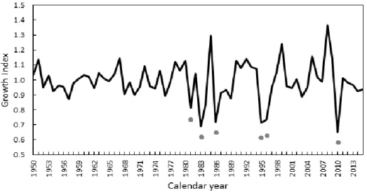
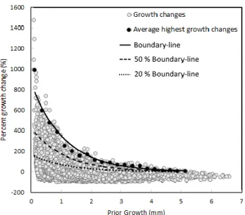
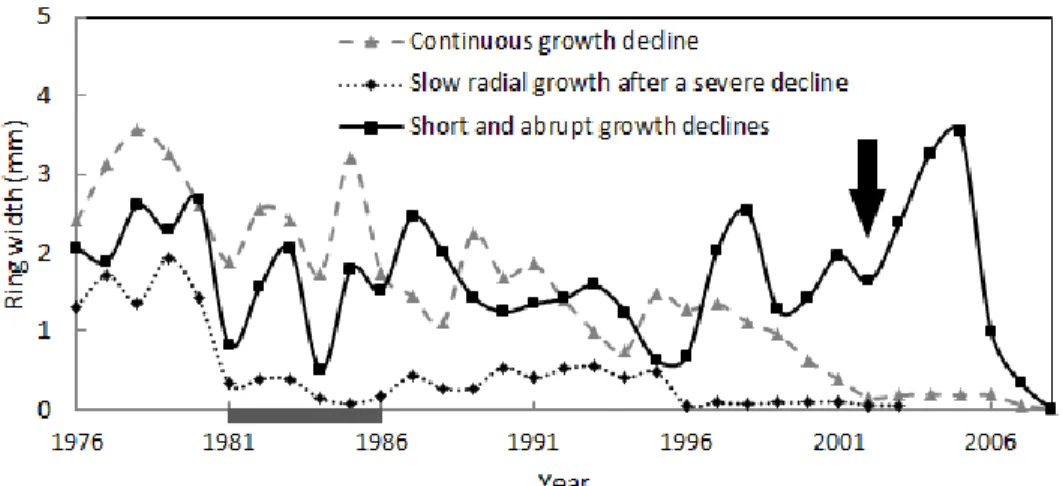
Figure 1.1 Effects of A) DBH and B) distance to nearest skid trail on mean predicted harvest probabilities for all species group. ... 20 Figure 1.2 Mean predicted annual basal area increment during the 10-year after cutting (𝐵𝐴𝐼10) as a function of the ln transformation of the competition index before cutting ln(𝐶𝐼𝑏𝑐).. ... 23 Figure 1.3 Effects of A) the competition index before cutting and B) species group on the mean predicted survival probabilities ... 24 Figure 2.1 Age-standardized master chronology from the mean radial growth of 38 dominant sugar maple trees (r = 0.90). ... 44 Figure 2.2 Percent growth changes (PGC) measured during 10-year periods after a given year of interest as a function of the 10-year radial growth measured before this given year for sugar maple trees located in southern Quebec, Canada.. ... 46 Figure 2.3 Three different ring series patterns that were observed prior to tree death: i) long periods of continuous growth decline interspersed with small pulses of radial growth that ended with tree death, ii) long periods of slow radial growth after a severe decline, and iii) short and abrupt growth decline in years following selection cutting ... 49 Figure 2.4 Effects of explanatory variables on mean predicted mortality probabilities ... 51 Figure 2.5 Percentage of (a) live trees (n=86) and (b) dead trees (n=25) for which release events were detected in each decade since 1950. ... 52 Figure 2.6 Effects of competition index a) and tree vigour at the time of selection cut; b) on mean predicted growth release probabilities after selection cutting. ... 53 Figure 3.1 Method for determining the crown density (CDEN), i.e. the amount of crown branches, foliage, and reproductive structures that blocks light visibility through the projected crown outline ... 72 Figure 3.2 Mean observed A) basal area increment and B) growth efficiency as function of the DBH class and the crown density (CDEN) for sugar maple trees.. ... 77 Figure 4.1 Bootstrapped response function coefficients computed between sugar maple residual chronologies and the monthly climatic variables over the 1963-2015 period for A) temperature and B) precipitation in Estrie and C) temperature and D) precipitation in Beauce ... 100 Figure 4.2 Non-stationary relationship between sugar maple growth and monthly climatic predictors in Estrie (A) and Beauce (B) regions. ... 101 Figure 4.3 Average growth index chronologies (A) in Estrie (nbr = 21, EPS = 0.89), and (B) in Beauce (nbr = 16, EPS = 0.87). Average ring-width (mm) chronologies (C) in Estrie and (D) in Beauce. E) Growth sensitivity index calculated over a 5-year segment from all individual tree-ring series (E) in Estrie and (F) in Beauce.. ... 103 Figure 4.4 Mean observed growth index as a function of the accumulated GDD during thaw-freeze and drought event in Estrie (A; C) and Beauce (B; D), respectively. ... 104 Figure 4.5. Mean predicted abrupt growth decline probability as affected by accumulated GDD during thaw-freeze and drought event in Estrie (A; C) and Beauce (B; D), respectively ... 105

(10)

Liste des tableaux

Table 1.1 Pre-harvest descriptive characteristics of trees (mean ± standard deviation, minimum - maximum) according to species group from the 23 permanent sample plots for stems with DBH > 9 cm... 14 Table 1.2 Model selection results for the five best regression models predicting the harvest probability in selection cuts. ... 20 Table 1.3 Model selection results for the five best regression models predicting the basal area growth response of trees during a 10-year period following selection cuts.. ... 21 Table 1.4 Model-averaged parameter estimates and their 95 % confidence interval (CI) computed for the basal area increment and the survivals models. ... 22 Table 1.5 Model selection results for the five best regression models predicting the probability of tree survival following selection cutting. ... 23 Table 2.1 Definitions of defects characterizing low-vigour trees according to the classification system of Majcen et al. (1990) as adapted by Guillemette et al. (2008). ... 43 Table 2.2 Statistics of the 5 best simple and multiple regression models predicting the probability of tree mortality following selection cutting. ... 50 Table 2.3 Statistics of the best models predicting the probability of growth release occurrence following selection cutting. ... 52 Table 3.1 Number of sugar maple and yellow birch trees sampled in the 35 PSPs by diameter class and categorical defect categories ... 75 Table 3.2 Model selection result from the three distinct steps (univariate, bivariate and multivariate models) predicting the basal area increment of sugar maple trees. ... 76 Table 3.3 Model selection result from the three distinct steps (univariate, bivariate and multivariate models) predicting the growth efficiency of sugar maple trees. ... 78 Table 3.4 Model-averaged parameter estimates and their 95 % confidence interval (CI) for sugar maple computed from the five best multivariate models.. ... 79 Table 3.5 Model selection result from the three distinct steps (univariate, bivariate and multivariate models) predicting the basal area increment of yellow birch trees. ... 80 Table 3.6 Model selection result from the three distinct steps (univariate, bivariate and multivariate models) predicting the growth efficiency of yellow birch trees. ... 81 Table 3.7 Model-averaged parameter estimates and their 95 % confidence interval (CI) for yellow birch computed from the five best multivariate models. ... 82 Table 4.1 Severe climatic events detected for the period 1963-2015 for the two study regions. GDD is the maximum cumulated growth degree-days during a thaw-freeze/drought event and days is the maximum cumulated days during a thaw-freeze/drought event.. . 102

(11)

Remerciements

Je tiens à remercier sincèrement mon directeur de recherche, David Pothier, pour sa confiance et pour m’avoir donné la chance de poursuivre mes études graduées sur un sujet qui me passionne. Merci pour ta disponibilité et ta rigueur qui m’ont permis d’avancer rapidement et de me développer comme chercheur. Je veux également remercier mon co-directeur de recherche, Alexis Achim, qui a grandement contribué à ce projet et à ma formation. Merci pour ton ouverture, ton enthousiasme, ta créativité et pour toutes les opportunités que tu m’as données pour que je me développe comme chercheur. Ensemble, vous avez été d’un grand support dans mes travaux et votre camaraderie a rendu mon expérience fort agréable. J’ai eu énormément de plaisir à travailler avec vous. Je veux également vous remercier de m’avoir permis de dévier à quelques reprises d’un parcours académique traditionnel, en me permettant de réaliser des projets parallèles à ma thèse qui étaient très importants à mes yeux.

Ce projet de recherche n’aurait pas été possible sans la participation de notre partenaire industriel Domtar. J’aimerais remercier André Gravel, Patrick Cartier, Élise Jolicoeur, Éric Lapointe, Steeve Reynolds ainsi que Christian Guimont pour leur support et leur confiance. Vos conseils et votre aide technique ont grandement facilité ma progression.

Je souhaite remercier Ann Delwaide de m’avoir accompagné patiemment dans mes analyses de laboratoire et pour tous ses précieux conseils. Ton enseignement a fortement contribué à mon désir de faire un passage accéléré au doctorat. Merci également à Évelyne Thiffault de m'avoir partagé ton enthousiasme pour le monde de la recherche alors que je n’étais qu’un étudiant au premier cycle.

Un grand merci également à Éloïse Dupuis, Alexandre Morin-Bernard, Félix Poulin, Marie-Laure Lusignan, Émilie St-Jean et Édouard Moreau pour votre aide sur le terrain. Un merci tout spécial à mon ami Michel Poudrier pour son aide technique en programmation. Ce projet n’aurait pas été possible sans votre aide précieuse.

J’aimerais aussi remercier les membres de mon comité de thèse qui ont accepté d’examiner ce document, soit Christian Messier, Filip Havreljuk et Jean-Claude Ruel. Merci pour vos commentaires constructifs.

(12)

Enfin, je veux remercier mes parents et ma famille pour leur support inconditionnel dans mon cheminement académique. Jamais il ne m’aurait été possible d’atteindre un niveau d’accomplissement aussi élevé sans votre aide et sans vous avoir eu comme exemple. Je vous remercie du fond du cœur. Je termine en remerciant ma douce moitié, Catherine, pour son support et surtout, de me donner les meilleures raisons du monde de décrocher de mes recherches et de prendre des pauses du travail.

(13)

Avant-propos

Insertion d’articles

Cette thèse est composée de quatre chapitres rédigés en anglais et présentés sous forme d’articles scientifiques. En tant que candidat au doctorat et premier auteur, j'ai effectué la revue de littérature, établi les objectifs de recherche, réalisé et encadré l'échantillonnage sur le terrain, réalisé les analyses statistiques et l’interprétation des résultats et rédigé l’ensemble des articles scientifiques.

Chapitre 1

Moreau, G., Achim, A., & Pothier, D. (2020). Growth and survival dynamics of partially cut northern hardwood stands as affected by precut competition and spatial distribution of residual trees. Forestry: An International Journal of Forest Research. 93(1), 96-106 (Soumis le 1 mars 2019, accepté le 26 juillet 2019, publié en ligne le 11 octobre 2019)

Chapitre 2

Moreau, G., Achim, A., & Pothier, D. (2019). A dendrochronological reconstruction of sugar maple growth and mortality dynamics in partially cut northern hardwood forests. Forest ecology and management, 437, 17-26. (Soumis le 12 novembre 2018, accepté le 16 janvier 2018, publié le 22 janvier 2019)

Chapitre 3

Moreau, G., Achim, A., & Pothier, D. (2020). Relevance of stem and crown defects to estimate tree vigour in northern hardwood forests. Forestry: An International Journal of Forest Research. (Soumis le 4 septembre 2019, accepté le 27 janvier 2020, publié en ligne le 5 mars 2020)

Chapitre 4

Moreau, G., Achim, A., & Pothier, D. (2020). An accumulation of climatic stress events has led to years of reduced growth for sugar maple in southern Quebec, Canada. Ecosphere. (Soumis le 31 janvier 2020, accepté le 14 avril 2020)

(14)

Coauteurs des chapitres

La rédaction de cette thèse de doctorat a été supervisée par David Pothier, directeur de thèse, et Alexis Achim, codirecteur de thèse. Ils sont les coauteurs de tous les chapitres puisqu’ils ont supervisé les travaux de recherche et ont participé à la rédaction des articles scientifiques.

David Pothier : Département des sciences du bois et de la forêt, Université Laval, 2405 rue de la Terrasse, Québec, Québec, Canada. G1V 0A6. Courriel : David.Pothier@sbf.ulaval.ca Alexis Achim : Département des sciences du bois et de la forêt, Université Laval, 2405 rue de la Terrasse, Québec, Québec, Canada. G1V 0A6. Courriel : alexis.achim@sbf.ulaval.ca

(15)

Introduction

Les forêts feuillues de l’Amérique du Nord couvrent de grandes superficies du sud-est du Canada au nord-est des États-Unis et se situent principalement à proximité de zones densément peuplées, de la région des Grand-Lacs jusqu’à l’océan Atlantique (Bailey 1983). La proximité des usines de transformation et des marchés, ainsi que la grande valeur des bois feuillus pour les secteurs de transformation primaire donnent une importance économique considérable à la forêt feuillue (MFFP 2017). Uniquement au Québec, entre 2011 et 2017, la consommation totale de feuillus durs par les secteurs du déroulage, du sciage, des panneaux, des pâtes et papiers et du bois de chauffage était en moyenne de 6 665 000 m³/an (MFFP 2017).

Le régime de perturbations naturelles de ces forêts est dominé par des perturbations partielles du couvert forestier, dont l’intervalle de retour relativement rapide (50-200 ans) produit une mosaïque de peuplements caractérisés par des structures irrégulières et inéquiennes (Lorimer & Frelich 1994; Seymour et al. 2002; Raymond et al. 2009). On retrouve au sein de ces structures complexes les attributs de forêts matures, tels que plusieurs cohortes d’arbres provenant de différentes perturbations plus ou moins récentes, une grande variation de la taille et de l’âge des arbres, ainsi qu’une distribution spatiale hétérogène de ces derniers au sein des peuplements (Raymond et al. 2009). Bien que dominées par l’érable à sucre (Acer saccharum Marsh.), ces forêts sont composées de plusieurs espèces d’arbres dont les caractéristiques écologiques telles que la longévité, la tolérance à l’ombre et la vitesse de croissance varient entre elles (Lorimer & Frelich 1994; Seymour et al. 2002). Cette irrégularité dans la composition forestière et la structure des peuplements engendre une dynamique de croissance et de mortalité complexe, résultant d’une répartition hétérogène des ressources entre les individus de différentes espèces et de leur efficacité à utiliser ces ressources (Pothier 2019).

Pour reproduire les effets du régime de perturbations naturelles, les peuplements feuillus sont principalement exploités à l'aide de la coupe de jardinage qui vise à maintenir la structure irrégulière ou inéquienne du peuplement, à promouvoir la régénération des espèces désirées, à améliorer la vigueur générale du peuplement et à fournir un rendement soutenu en bois de haute qualité (Arbogast 1957; Majcen 1996; Nyland 1998; Raymond et al. 2009). À chaque cycle de récolte, environ un tiers des arbres est abattu, libérant ainsi les arbres résiduels de certains de leurs concurrents directs. Au Québec, la coupe de jardinage

(16)

a pris de l’ampleur au début des années 1990, succédant à la coupe à diamètre limite qui est reconnue pour avoir diminué le potentiel de production du bois de qualité par la dégradation des peuplements résiduels et la prolifération d’espèces indésirables (Guillemette et al. 2008). Bien que la coupe de jardinage ait donné des résultats prometteurs après son application dans des blocs expérimentaux (plus grand accroissement net dans les peuplements traités que dans les témoins), les résultats provenant de son application dans un contexte industriel ont été beaucoup moins convaincants (Majcen 1996; Bédard & Brassard 2002). Ces derniers résultats ont fait ressortir une productivité environ 40 % plus faible que celle anticipée en raison d’un taux de mortalité deux fois plus élevé que celui observé dans les dispositifs expérimentaux (Bédard & Brassard 2002). Plus récemment, on a également constaté une grande variation de la mortalité et de l’accroissement des arbres entre les régions et les conditions de croissance (e.g. Forget et al. 2007; Nolet et al. 2007; Fortin et al. 2008; Hartmann et al. 2009; Guillemette et al. 2008; Martin et al. 2014). Ce constat soulève plusieurs questions sur les facteurs qui prédisposent certains arbres à réagir positivement ou négativement à une coupe de jardinage. Bien que des études aient documenté les causes potentielles de mortalité des arbres résiduels (e.g. Caspersen 2006; Martin et al. 2014), la compréhension et la quantification de l’effet de ces facteurs sur la structure et la dynamique de croissance des peuplements résiduels restent à préciser. En général, la création d’ouvertures dans le couvert forestier stimule la croissance des arbres situés à leur proximité en raison d’une diminution de la compétition et de l’augmentation de la disponibilité des ressources (Nowacki & Abrams 1997; Black & Abrams 2003; Jones & Thomas 2004). La réaction de croissance en diamètre devrait augmenter proportionnellement au degré d’ouverture du couvert forestier (Jones & Thomas 2004). Cependant, l’ouverture du couvert forestier dans le cadre de coupes de jardinage mécanisées peut aussi produire une compaction des sols et ainsi causer des dommages aux racines primaires des arbres, ce qui limite l’absorption d’eau et de nutriments (Hartmann et al. 2009). Ces dommages peuvent compromettre le développement des racines dans les années suivant la coupe, provoquer un stress hydrique et créer des portes d’entrée pour différents pathogènes (Hartmann et al. 2009). En plus de la compaction des sols, les coupes mécanisées peuvent aussi causer différents dommages aux arbres résiduels, variant du bris et de la perte de branches jusqu’à de larges abrasions sur le tronc et les racines (Nyland 1998; Hartmann et al. 2009). Ces blessures créent des portes d’entrée pour les pathogènes qui dégradent et annellent partiellement les arbres, ce qui réduit la croissance diamétrale.

(17)

En conséquence, la réaction de croissance des arbres résiduels à la suite des coupes peut être diminuée et leur taux de mortalité peut augmenter (Caspersen 2006; Hartmann et al. 2009; Martin et al. 2014). L’effet simultané des impacts positifs et négatifs des coupes de jardinage mécanisées rend difficilement prévisible la réaction de croissance des arbres, ce qui peut expliquer la grande variabilité des résultats obtenus à ce jour (Hartmann et al. 2009).

Les études ayant tenté de déterminer les causes de mortalité à la suite d’une récolte partielle ont principalement utilisé une approche post-mortem dans laquelle une cause « probable » était déduite d'un examen des caractéristiques physiques des arbres morts (Nolet et al. 2007; Martin et al. 2014; Guillemette et al. 2017). Puisque la mortalité est un phénomène complexe qui est généralement le résultat cumulatif de plusieurs causes, c’est-à-dire des facteurs incitatifs et des facteurs contributifs (Manion 1981), cette approche post-mortem peut facilement confondre les causes et les effets, en plus de n’identifier qu’une cause de mortalité. Par exemple, lorsque le chablis est identifié comme cause de mortalité, il est possible que l’arbre soit en réalité mort sur pied pour ensuite être renversé par le vent. Pour préciser cette approche post-mortem, l’utilisation de séries de croissance interdatées pourrait permettre d’étudier rigoureusement les patrons de croissance précédant la mortalité, de manière à déterminer avec précision les années de déclin de croissance ainsi que l’année de la mort des arbres. En effet, les récents progrès des méthodes dendrochronologiques ont fourni des observations précises sur les réactions de croissance et de mortalité des arbres à la suite de perturbations naturelles (Bigler & Bugmann 2004; Cailleret et al. 2017). Ces études ont démontré que la majorité des événements de mortalité sont associés à une période de réduction de croissance sur plus de 20 ans précédant la mort des arbres, de sorte que de meilleures prévisions de la mortalité peuvent être obtenues en considérant les tendances de croissance radiale à long terme (Bigler & Bugmann 2004; Cailleret et al. 2017). Pourtant, à notre connaissance, les tendances de croissance radiale à long terme n’ont jamais ou très peu été prises en compte par les études portant sur la dynamique temporelle et les causes de mortalité induites par des coupes de jardinage dans les forêts composées de feuillus nordiques (Hartmann & Messier 2008).

Un autre facteur d’incertitude pouvant expliquer une partie de la variation des résultats obtenus à la suite de coupes de jardinage est l’utilisation de systèmes de classification de la vigueur des arbres qui n’ont, encore à ce jour, que partiellement été validés de manière empirique. Ces systèmes de classification visent à estimer la vigueur des arbres pour guider

(18)

les opérations de martelage en se basant sur les caractéristiques du houppier (Schomaker 2007), de l’écorce (OMNR 2004), des dommages pathologiques et mécaniques (OMNR 2004; Boulet 2007; Pelletier et al. 2016) et de la morphologie de l’arbre (Pelletier et al. 2016). La vigueur d’un arbre a été définie à la fois comme étant son potentiel de croissance (OMNR 2004; Pelletier et al. 2016) ou sa probabilité de mortalité durant la prochaine rotation de coupe (Boulet 2007).

Au Québec, le système de classification de la vigueur des arbres lors du martelage (Boulet 2007) a été mis au point en réaction à la croissance décevante des peuplements traités par des coupes de jardinage dans un contexte industriel (Bédard & Brassard 2002). Ce système de classification estime la vigueur des arbres pour ainsi former quatre priorités de récolte (M-S-C-R) lors du martelage précédant une coupe de jardinage (Boulet 2007).

i. Mourir: Tige très défectueuse, qui risque de se renverser, de se rompre ou de mourir sur pied avant la prochaine rotation (Priorité de récolte 1).

ii. Survie : Tige défectueuse en perdition dont le volume de bois risque de diminuer en raison de la carie, mais dont la survie n’est pas menacée avant la prochaine rotation (Priorité de récolte 2).

iii. Conserver : Tige peu défectueuse à conserver, dont le volume de bois marchand ne risque pas de se dégrader avant la prochaine rotation (Priorité de récolte 3).

iv. Réserve : Tige saine en réserve qui constitue le capital forestier de premier choix (Priorité de récolte 4).

Bien que ce système de classification soit appuyé par des observations préliminaires (Boulet & Landry 2015), certaines études empiriques ont conclu que la capacité du système à prévoir le risque de mortalité des arbres est globalement faible (Hartmann et al. 2008; Guillemette et al. 2015). En général, ces études ont mis en évidence que les arbres avec la plus haute priorité de récolte (M) ont bel et bien un risque de mortalité plus élevé que ceux des autres classes. Toutefois, les différences de risque de mortalité entre les autres classes de priorité de récolte (S, C et R) ne se sont pas statistiquement distinguées. Récemment, Moreau et al. (2018a) ont utilisé un indice de vigueur quantitatif fondé sur la production annuelle de bois par unité de surface foliaire, aussi appelé indice d’efficacité de croissance (Waring et al. 1980), pour valider le système de classification MSCR. Or, l’indice d’efficacité

(19)

de croissance n’a pu être significativement relié aux classes de priorité de récolte MSCR (Moreau et al. 2018a). Cette absence de lien significatif indique que le système de classification par priorité de récolte est peu relié à la vigueur réelle des arbres et qu’il est donc peu probable que son application soit accompagnée par des gains importants de vigueur pour les peuplements traités par coupe de jardinage.

Par leur nature empirique, les études traditionnelles en sylviculture ont été construites de manière à observer les tendances de croissance à la suite de pratiques passées, afin d’ajuster les stratégies d’aménagement actuelles et futures. Cette approche fait le postulat que les conditions de croissance passées reflèteront avec précision le potentiel de croissance futur. Or, dans les dernières décennies, l’augmentation soutenue de la température annuelle ainsi que la sévérité et la fréquence des stress climatiques ont eu un impact direct sur la dynamique des écosystèmes forestiers (Bell et al. 2004; Iverson et al. 2008; Allen et al. 2010; Dai 2013; Zhang et al. 2018). En Amérique du Nord, on a observé un changement de composition forestière favorisant les espèces à croissance lente qui sont mieux adaptées aux stress climatiques, modifiant ainsi la dynamique de croissance et la captation de carbone (Zhang et al. 2018). Ces observations mettent en évidence certaines limites du postulat proposant que les conditions de croissance passées sont garantes de celles du futur, et pourraient expliquer une partie de la variation des résultats obtenus à la suite de coupes de jardinage. Étant donné qu’une augmentation des stress climatiques est attendue dans les prochaines années, les changements appréhendés de dynamique de croissance ajoute de l’incertitude au maintien de la productivité forestière à long terme (Zhang et al. 2018; SCAF 2018) et à l’efficacité de l’application des traitements sylvicoles. Afin d’anticiper l’effet des changements climatiques sur les écosystèmes forestiers et, ultimement, mettre en œuvre des mesures adaptatives à l’aménagement actuel, il apparaît impératif de raffiner notre compréhension de la vulnérabilité des espèces feuillues aux différents stress climatiques (Allen et al. 2015; D’Amato et al. 2013; Nolet & Kneeshaw 2018). Malgré ce constat, à ce jour, nous connaissons mal les relations entre la croissance de nos espèces feuillues et les conditions climatiques (Tardif et al. 2001; Bishop et al. 2015). De plus, l’effet des différents stress climatiques sur la dynamique de croissance des forêts feuillues n’a encore jamais été inclus dans des modèles de prévision en Amérique du Nord.

(20)

Démarche méthodologique

L’objectif général de ce projet de recherche est d’améliorer les prévisions de la croissance et de la mortalité des arbres feuillus à partir d’une meilleure évaluation de leur potentiel de croissance sur pied et de leur sensibilité aux conditions climatiques. L’approche proposée par cette étude vise à améliorer l’évaluation visuelle des arbres pour refléter adéquatement leur potentiel de croissance en établissant des liens étroits entre leurs caractéristiques morphologiques, leur vigueur et leur sensibilité aux conditions climatiques. Les données utilisées pour l’ensemble de ce projet proviennent de 36 placettes échantillons permanentes (PEP) couvrant deux régions du sud du Québec, soit l’Estrie et la Beauce. Le projet de recherche est divisé en quatre chapitres distincts.

Le premier chapitre de la thèse a comme objectifs spécifiques i) d’évaluer l’impact de la distribution spatiale des arbres produite par le passage de la machinerie durant la coupe de jardinage sur la réaction de croissance et le taux de survie et des arbres résiduels et ii) d’évaluer l’importance de l’environnement compétitif avant et après la coupe sur la réaction de croissance et le taux de survie. Un modèle de prévision de la probabilité de récolte, de l’accroissement et de la mortalité des arbres en fonction de leur répartition spatiale au moment du traitement a été mis au point. Un total de 23 PEP a été échantillonné afin de reconstruire l’environnement de croissance de 455 arbres, dont 97 ont été récoltés et 68 sont morts suivant l’application du traitement.

L’objectif du second chapitre est d’évaluer l’effet des tendances de croissance antérieures sur le taux de mortalité et la réaction de croissance des arbres à la suite d’une coupe de jardinage. Plus précisément, ce chapitre a testé les hypothèses de recherche suivantes : i) la mortalité post-récolte est généralement précédée par un déclin de croissance progressif durant les décennies précédant la coupe (> 20 ans), plutôt que par une chute marquée de la croissance suivant l’application du traitement, et ii) une croissance radiale limitée durant une longue période avant la coupe (> 20 ans) va diminuer la probabilité d’avoir une hausse de croissance à la suite d’une coupe de jardinage. L’étude des tendances de croissance antérieures a été faite à l’aide de 112 séries de croissance inter-datées réalisées sur des érables à sucre (86 vivants et 26 morts) et couvrant une période de 65 ans, de manière à caractériser les patrons de croissance pré-récolte et à identifier les caractéristiques morphologiques (i.e. taille, vigueur) qui prédisposent certains arbres à avoir une hausse de croissance ou à mourir à la suite d’une coupe de jardinage.

(21)

Le troisième chapitre de la thèse vise à identifier les défauts apparents du tronc et du houppier des arbres qui sont significativement reliés à leur vigueur actuelle. Pour ce faire, nous avons réalisé une analyse des relations entre deux indices de vigueur reconnus et une gamme complète de caractéristiques du tronc et du houppier répertoriés dans trois systèmes de classification de la vigueur utilisés en Amérique du Nord. Un total de 336 érables à sucre et 84 bouleaux jaunes ont été échantillonnés. Les analyses statistiques ont été faites avec parcimonie, de manière à identifier l’assemblage de défauts le plus simple pour estimer la vigueur actuelle des arbres.

L’objectif du quatrième chapitre est de quantifier l’effet des conditions climatiques sur la dynamique de croissance de l’érable à sucre. Ainsi, ce chapitre vise à i) quantifier de manière empirique l’effet de deux types d’événements climatiques sévères (sécheresse et gel-dégel) sur la dynamique de croissance de l’érable à sucre, et ii) comparer l’effet de ces événements climatiques sévères à celui des tendances climatiques mensuelles. Une chronologie de référence a été construite pour chacune des deux régions couvertes par notre jeu de données (l’Estrie et la Beauce) et l’effet du climat sur la croissance a été analysé sur une période de plus de 50 ans.

Les résultats de ce projet de recherche devraient permettre de mieux comprendre la dynamique de croissance des arbres à la suite d’une coupe de jardinage mécanisée et ainsi améliorer l’évaluation visuelle des arbres de façon à refléter adéquatement leur potentiel de croissance au moment de la récolte. Cette approche devrait aider à maximiser la production de bois de qualité en forêt feuillue en conservant les forts contributeurs à la croissance globale des peuplements. De plus, nos résultats devraient permettre de mieux comprendre l’impact des conditions climatiques sur la dynamique de croissance de l’érable à sucre, une étape essentielle pour intégrer l’effet potentiel des changements climatiques sur la croissance à long terme de nos peuplements feuillus.

(22)

1. Chapitre 1

Growth and survival dynamics of partially cut

northern hardwood stands as affected by precut

competition and spatial distribution of residual

trees

(23)

1.1. Abstract

Modelling growth and survival dynamics after partial harvesting must take account of the heterogeneous spatial pattern of residual trees that results from the presence of machinery trails. We used data from 23 permanent sample plots in northern hardwood stands to reconstruct the growing environment of individual trees before and after partial harvesting. We modelled harvest probability, growth response and survival probability using a complementary set of explanatory variables that was assembled to reflect the spatial distribution of trees and skid trails prior to and after harvest. Results showed that the distribution of harvested trees was concentrated in skid trails and in their close vicinity. However, this spatial pattern had no significant effect on either the post-cut basal area increment (BAI) or the survival of residual trees. BAI and survival of individual trees were both mostly related to the competitive environment prior to harvest, while post-cut changes in competitive environment had only a marginal effect on growth and survival dynamics. We conclude that selection cuts did not substantially increase the growth and survival of residual trees, likely because tree removal was mostly concentrated near skid trails, where the negative effects of machinery access were highest.

(24)

1.2. Résumé

Un total de 23 placettes échantillons permanentes ont été échantillonnées afin de reconstruire l’environnement de croissance avant et après l’application d’une coupe de jardinage. La probabilité de récolte, la réaction de croissance et la probabilité de survie ont été modélisées en utilisant un assemblage de variables reflétant la distribution spatiale des arbres et des sentiers de débardage. Nos résultats ont montré que le prélèvement des arbres a été concentré à l’intérieur et aux abords des sentiers de débardage. La croissance et la survie des arbres résiduels étaient principalement liées à l’environnement compétitif avant la coupe. À l’inverse, la diminution de l’environnement compétitif induit par la coupe n'avait qu'un effet marginal sur la croissance et la survie des arbres résiduels. Nous concluons que les coupes de jardinage n'ont pas augmenté la croissance et la survie des arbres en raison d’une récolte concentrée à l’intérieur et aux abords des sentiers de débardage.

(25)

1.3. Introduction

The natural disturbance regime in northern hardwood forests is driven by small canopy gaps created by the death of one to several dominant trees (Lorimer & Frelich 1994). Natural senescence, wind, pathogens and insect herbivory are the main mortality agents whose average return interval of 50-200 years generally results in multi-cohort, uneven-aged stands dominated by shade-tolerant species (Seymour et al. 2002). To mimic this natural mortality regime, northern hardwood stands are mainly managed using selection cuts. In recent decades, these have been applied as part of the ‘selection’ silvicultural system that aims to maintain the stand’s uneven-aged structure, to promote the regeneration of desired species, to improve the overall stand vigour, and to provide a sustained yield of high-quality timber (Arbogast 1957; Majcen 1996; Nyland 1998). At each harvest cycle, about one third of the trees are removed and most residual trees should at least be partly released from direct competitors.

Several studies have been conducted to understand the factors that influence growth and mortality dynamics after such selection cuts. In general, gap creation stimulates the radial growth of residual trees by reducing competition and improving resource availability (Nowacki & Abrams 1997; Jones & Thomas 2004; Dyer et al. 2010). However, gaps created by mechanized selection cuts may also be associated with soil disturbance and compaction, in addition to damage to the roots and trunk of residual trees (Grigal 2000; Seablom & Reed 2005; Thorpe et al. 2008). Such effects may increase mortality and mitigate the growth response of surviving trees following selection cuts (Caspersen 2006; Thorpe et al. 2008; Hartmann et al. 2009; Martin et al. 2014). The concurrent positive and negative influences of harvest gaps yield uncertainty regarding the net stand-level response to selection cuts.

Because all trees are harvested in trails used for the machinery access, residual trees are typically clustered, which in turn leads to an uneven distribution of resources among them (Boivin-Dompierre et al. 2017). Consequently, tree growth responses are also likely to follow a spatial pattern that depends on trail width and spacing (e.g. Hartmann et al. 2009; Boivin-Dompierre et al. 2017). Information about the spatial distribution of trees and skid trails within a stand would thus be useful to help predict the growth of residual trees after selection cutting. In northern hardwood forests, only a few studies have used the spatial distribution of trees relative to skid trails as predictors of the tree growth response after selection cuts, and they were all conducted in the same study site (e.g. Hartmann et al. 2008; Hartmann &

(26)

Messier 2008; Hartmann et al. 2009). While Hartmann et al. (2008) and Hartmann & Messier (2008) found no relationship between the growth response of sugar maple trees and the distance to a skid trail, Hartmann et al. (2009) showed a negative impact of the machinery passage on tree growth as far as 12 m from skid trails. In contrast, after mechanized group-selection openings whose sizes varied from 50 to 400 m2_{, Jones and Thomas (2004) and}

Dyer et al. (2010) found higher annual diameter increment for trees located at the gap edge. Because the negative impact of harvesting operations mainly influences trees close to skid trails, post-cut mortality is also likely to follow a similar spatial pattern in years following partial harvest (Thorpe et al. 2008). In a boreal forest, the proximity to a skid trail was found to have a major impact on the cumulative mortality of residual black spruce (Picea mariana (Mill.) B.S.P.) trees during the first decade after harvest (Thorpe et al. 2008). However, such spatial mortality dynamics have yet to be quantified in northern hardwood forests.

In addition to the spatial pattern produced by mechanized partial harvesting, the growth response of trees could be affected by other factors such as stem size (Jones & Thomas 2004; Jones et al. 2009) and their social status within the canopy prior to harvest (Latham & Tappeiner 2002; Hartmann et al. 2009; Dyer et al. 2010). Indeed, trees occupying a dominant canopy position prior to the cut were likely under less competitive pressure, and therefore growing faster, than subordinate trees. Consequently, a selection cut may not produce major changes in light availability for large, dominant trees, a fact that could limit their growth response (Dyer et al. 2010) and the effect on their survival probability. Conversely, trees that were subject to intense competition for light before selection cutting could respond markedly to the treatment due to the noticeable improvement in their competitive environment (Black & Abrams 2003). However, these growth trends among trees of different social status and competitive environment have rarely been considered, presumably because information about competition between trees before harvest is rarely available.

In this study, we used data from 23 permanent sample plots (PSP) that were established in different northern hardwood stands to reconstruct the growing environment of individual trees before and after selection cutting. Our main objective was to evaluate the effect of the spatial distribution of trees relative to skid trails at time of harvest on their post-cut growth and survival dynamics. To consolidate our analysis, we modelled harvest probability, growth response and survival probability using a complementary set of candidate explanatory variables. The specific objectives of the study were to: i) assess the impact of the spatial

(27)

pattern produced by selection cuts on the tree growth response and post-cut survival and ii) evaluate the importance of the pre- and post-cut competitive environments on the growth response and survival of individual trees to selection cuts. Obtaining improved knowledge about growth and survival of trees and their spatial distribution patterns after mechanized selection cutting is of operational and ecological interest, and is key to the long-term sustainability of northern hardwood forests managed under the selection silvicultural system.

1.4. Material and methods

1.4.1. Sampling sites

The study area was located on private woodlots owned by Domtar Corporation in southern Quebec, Canada (45◦31’-45◦57’N, 71◦23’-70◦33’W) and encompasses both the eastern sugar maple-American basswood and the eastern sugar maple-yellow birch bioclimatic subdomains (Saucier et al. 2009). The first subdomain is characterized by mean annual temperatures between 4 and 5 °C and mean annual precipitation between 1000 and 1150 mm, with a growing season of 165 to 180 days. The second subdomain is characterized by mean annual temperatures between 2.5 and 4 °C and mean annual precipitation between 915 and 1100 mm, with a growing season of 145 to 165 days (Saucier et al. 2009). The topography of both subdomains is characterized by hills and slopes and the main surface deposits are shallow or deep tills (Grondin et al. 2007). The sampling sites were located in uneven-aged northern hardwood stands dominated by sugar maple (Acer saccharum Marsh.), followed by yellow birch (Betula alleghaniensis Britt.) and red maple (Acer rubrum L.), with minor components of American beech (Fagus grandifolia Ehrh.), black cherry (Prunus serotina Ehrh.), basswood (Tilia americana L.), hornbeam (Ostrya virginiana (Mill.) K. Koch), balsam fir (Abies balsamea (L.) Mill.), red spruce (Picea rubens Sargent) and Eastern hemlock (Tsuga canadensis (L.) Carr.).

1.4.2. Sample plots and treatments

From 1998 to 2003, 23 circular permanent sample plots (PSPs) of 400 m2_{were established}

randomly in stands representative of the regional site conditions, at least one year prior to the application of selection cuts. Within each of these PSPs, all trees with a diameter at breast height (DBH) > 9.0 cm were tagged. The selection cuts aimed at harvesting trees uniformly in a single operation and were conducted between 2002 and 2007. The long-term disturbance history of stands was unknown but there were no signs of cuts from previous years such as old stumps. Before cutting, stands were characterized by a mean density of

(28)

523 trees/ha, a mean basal area of 26 m2_{/ha, and a mean DBH of 26 cm (Table 1). The}

mean harvest rate in PSPs was 30 % (± 15 %) of the basal area. Trees were removed using feller-buncher harvesters working with a forwarder, a cable skidder or a grapple skidder. Skidding trails had a maximum width of 4 m

and were spaced about 20 m apart from edge

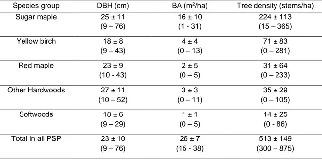
to edge. The selection cuts aimed to remove senescent trees and trees of low vigour from all species and DBH classes while maintaining an uneven-aged structure in the residual stand. Tree marking was conducted in eight of the 23 stands before harvest, in which cases it was applied according to a classification developed by Majcen et al. (1990). This classification assigns trees a survival probability until the next scheduled harvest based on pathological symptoms, mechanical damage and other visible defects. Then, based on a visual inspection of the stem, the classification system also assigns a quality grade that segregate trees with sawlog potential from trees with only pulpwood potential. This classification was referred to as the ‘VQ’ system in Delisle-Boulianne et al. (2014). In the 15 remaining stands, the selection of stems to be harvested was done by experienced harvester operators.

Table 1.1 Pre-harvest descriptive characteristics of trees (mean ± standard deviation, minimum - maximum) according to species group from the 23 permanent sample plots for stems with DBH > 9 cm. Pre-harvest values are estimated based on previous survey and diameter measurement of stumps and dead trees. BA is the basal area.

Species group DBH (cm) BA (m2_/ha) _{Tree density (stems/ha)}

Sugar maple 25 ± 11 (9 – 76) 16 ± 10 (1 - 31) 224 ± 113 (15 – 365) Yellow birch 18 ± 8 (9 – 43) 4 ± 4 (0 – 13) 71 ± 83 (0 – 281) Red maple 23 ± 9 (10 - 43) 2 ± 5 (0 – 5) 31 ± 64 (0 – 233) Other Hardwoods 27 ± 11 (10 – 52) 3 ± 3 (0 – 11) 35 ± 29 (0 – 105) Softwoods 18 ± 6 (9 – 29) 1 ± 1 (0 – 5) 14 ± 25 (0 - 86) Total in all PSP 23 ± 10 (9 – 76) 26 ± 7 (15 - 38) 513 ± 149 (300 – 875)

(29)

1.4.3. Data collection

The PSPs were inventoried periodically at a mean interval of five years with an additional survey being systematically conducted during the year that immediately followed the application of the selection cuts. At each survey, the species and DBH of all trees with a DBH > 9.0 cm were recorded. During the summer of 2016, we collected additional information in all 23 plots to reconstruct the pre- and post-harvest competitive environments of all trees within each PSP. To do so, we georeferenced the position of all trees that 1) were alive both at the time of the selection cuts and at the last measurement in 2016, 2) had died after the selection cut, and 3) were harvested (based on the location of their stump). To be able to quantify the competitive environment of trees at the edge of our PSPs, we also georeferenced live trees, dead trees and stumps within a 6-m strip around the perimeter of each plot. The Cartesian coordinates of each tree and stump were determined by measuring their distance (± 0.1 m) and azimuth relative to the plot centre using a hypsometer and a compass.

The same method was used to localize and map the skid trails that were closest to each plot. Skid trails were delimited based on a set of criteria proposed by Hartmann et al. (2009), i.e. i) the presence of openings in the forest canopy, ii) the presence of wounds at the base of trees, iii) the presence of ruts, iv) the presence of stumps, v) the absence of obstacles, and vi) the presence of saplings belonging to species that are usually associated with higher levels of light and soil disturbance. Only clearly identifiable trails were considered for further analysis. The GIS software ArcGIS 9.2 (Esri GIS and Mapping Software, Redlands, CA) was used to compute the distance of each tree to the closest skid trail section.

During the summer of 2016, we also remeasured the DBH (± 0.1 cm) of all trees with a DBH > 9.0 cm as well as the diameter of each stump at a height of 30 cm above the ground (DSH). To estimate the DBH of trees that were harvested during selection cutting operations, we developed relationships between DSH and DBH using measurements made on 384 trees of all species and randomly selected from four DBH classes (9.0-19.0, 19.1-29.0, 29.1-39.0, and ≥ 39.1). Finally, the radial growth history was assessed from increment cores sampled on all live trees at a height of 1 m above ground and oriented towards the plot centre. The sample cores were glued to wooden blocks before they were air dried and gradually sanded to allow a clear identification of the latewood boundaries. Annual rings

(30)

were then measured for a period of 10 years before and after selection cut with a Velmex micrometer (± 0.002 mm).

1.4.4. Competition index

The level of competition around each tree was calculated using the distance-dependent competition index (𝐶𝐼) proposed by Hegyi (1974):

𝐶𝐼 = 𝛴

_𝑖=1𝑛

𝑑

𝑖

⁄

(𝑑

× 𝑑𝑖𝑠𝑡

𝑖

)

[1]

where 𝑑𝑖 is the DBH (mm) of the ith neighbour

tree located at a distance of dist

i (m) from the

subject tree, and 𝑑 is the DBH of the subject tree. All values were computed from the inventory conducted during the year that followed each selection cut. Estimates of DBH values immediately after cut for trees located in the 6-m buffer strip around each plot were produced to adjust the pre- and post-cut CI calculation in each plot. This was achieved using a linear model relating the DBH measured immediately after cut (𝐷𝐵𝐻0) and that measured

in 2016 (𝐷𝐵𝐻1) for the sample trees located within the plots. The prediction equation (R2 =

0.93) was:

𝐷𝐵𝐻0= 0.91𝐷𝐵𝐻1− 1.42𝑇 + 2.22

[2]

where T is the number of years between the application of the selection cut and 2016. If the estimated DBH of trees that were located in the 6-m strip around each plot was lower than 9 cm at the time of the cut, this entry was simply removed from the dataset that was used to calculate CI. To determine the radius to calculate CI (from 2 to 6 m) that was best related to tree growth, we used a mixed-effects linear model with a plot-level random effect. Based on the Akaike’s information criterion (AIC), the mixed-effect model that best explained growth included the competition index that was computed over a 6-m radius. This radius was thus used in all subsequent analyses. To estimate the level of competition around each tree before harvest, we used the same method but also included in the calculations all trees that had died since the selection cut, including all harvested trees. For stumps located within the PSP, the DBH at the time of cutting (𝐷𝐵𝐻0) was estimated by Eq. 2 using the last DBH

measurement before cutting (𝐷𝐵𝐻1) and the number of years between the last survey and

the year of cutting (𝑇).

In addition to the competition index calculated before (𝐶𝐼𝑏𝑐) and after (𝐶𝐼𝑎𝑐) cutting, two

(31)

(RI) was firstly defined as the difference between 𝐶𝐼𝑏𝑐

and 𝐶𝐼

𝑎𝑐

, and secondly the relative

release index (RRI) was defined as input variables:

𝑅𝑅𝐼 = (𝐶𝐼

𝑏𝑐

− 𝐶𝐼

𝑎𝑐

) 𝐶𝐼

⁄

𝑏𝑐

[3]

1.4.5. Modelling harvest probability

The modelling process was performed using 455 sample trees of which 97 were harvested at the time of the selection cuts, 68 had died since their application, and 290 remained alive between selection cuts and 2016. Harvest probability was modelled at the tree level using a mixed effects logistic regression with a plot-level random effect. Only trees harvested outside skid trails were included in this model because the harvest of these trees is independent of the obligatory passage of the machinery, and results solely from the choice of the tree marker and/or the operator. Moreover, because the trees harvested in the skid trails would have been assigned a null distance, the inclusion of these trees in the model would have clearly led to the conclusion that harvesting was clumped. The candidate explanatory variables were the DBH at time of harvest, 𝐶𝐼𝑏𝑐, the distance of trees to the

nearest skid trail section, and tree species. Some of the species were poorly represented and so could not be individually taken into account in the model. Consequently, we used the following species groups: i) sugar maple (n = 263), ii) yellow birch (n = 102), iii) red maple (n = 46), iv) softwoods (balsam fir, red spruce, black spruce and Eastern hemlock, n = 19), and v) other hardwoods (American beech, black cherry, basswood and hornbeam, n = 42). The type of treatment (with or without tree marking) and its interaction with the other candidate variables were also included in the model.

1.4.6. Modelling the radial growth response

The radial growth response of individual trees to selection cuts was expressed through 𝐵𝐴𝐼10

(dm2_yr-1_{), and was also statistically modelled using a mixed-effects linear model with a}

plot-level random effect. In addition to the four competition indices described above, the distance to the nearest skid trail and the species group (five levels) were submitted to the models as candidate explanatory variables. The level of correlation between 𝐶𝐼𝑏𝑐 and 𝐶𝐼𝑎𝑐 prevented

their use in the same model. Also, to rigorously evaluate the importance of the pre-cut competitive environment on the tree growth response, we did not include tree DBH as a candidate variable in the analysis because of its strong correlation with 𝐶𝐼𝑏𝑐 (r = -0.57). A

square-root transformation was applied to 𝐵𝐴𝐼10 to produce a normal distribution of the

(32)

1.4.7. Modelling survival probability

The occurrence of mortality events after selection cutting was deduced using the periodic PSP surveys. At each survey, all dead trees were identified although the exact time of death since cutting could only be approximated. Several methods were developed to consider such interval-censored data using survival functions (Cox and Oakes 1984). These functions make it possible to treat a mortality event as a binomial variable that takes a value of 1 if a tree died and a value of 0 if a tree survived over a given time interval (e.g. Fortin et al. 2008; Guillemette et al. 2008). Survival probability was modelled at the tree level using the Cox proportional hazards model with the plot included as a frailty random term. This model describes the probability of an event or its hazard (the mortality of the tree) if the subject survived up to that particular time point (the next PSP survey). We also included the following candidate explanatory variables in the model: the four competition indices described above (i.e. 𝐶𝐼𝑏𝑐, 𝐶𝐼𝑎𝑐, RI, and RRI), the distance to the nearest skid trail section and the species

group. Once again, we did not include tree DBH in the analysis because of its strong correlation with 𝐶𝐼𝑏𝑐.

1.4.8. Model selection

To determine the best prediction models, all candidate variables were included successively in each prediction model while always avoiding the inclusion of highly correlated predictors. The resulting models were systematically compared to an intercept-only model (null model). The selection of the best growth, survival and harvest models was based on AIC value and AIC weight. If no model was clearly better (i.e., with an AIC weight over 90 %), a model averaging procedure was performed to compute unconditional 95 % confidence intervals for parameters of interest (Mazerolle 2006). Variable parameters with confidence intervals excluding zero were considered as good predictors (Mazerolle 2006). The delta AIC, the marginal and the conditional coefficient of determination (R2) were also computed, but used only to help describe the models. In the case of the survival model, we computed the pseudo-R2 related to the Cox survival analysis, which was based on the improvement in likelihood between the fixed fitted model and a model without predictor variables (null model) (see Therneau & Lumley 2014). Multiple comparisons were made on species groups when this variable was significant in the models. Preliminary analyses indicated that there was a logarithmic relationship between tree growth response and the variables 𝐶𝐼𝑏𝑐 and 𝐶𝐼𝑎𝑐.

Consequently, a log transformation was applied to these variables to keep a linear relationship, facilitate model fitting and meet the regression model assumptions. All

(33)

statistical analyses were performed in the R statistical programming environment (Version

3.5.1, R Core Team, 2018). We used the lme function of the nlme package (Pinheiro et al. 2017) to develop our linear mixed effects models. The coxph function of the survival package (Therneau & Lumley 2014) was used for the Cox proportional hazards model while the glmer function of the lme4 package (Bates et al. 2015) was used for the mixed effects logistic regression. Model selection based on AIC and multi-model inferences were performed using the AICcmodavg package (Mazerolle, 2017). Multiple comparisons were performed using the pairwise-survdiff function of the survival package (cox proportional hazards models) and the glht function of the multcomp package (Hothorn et al. 2019). To avoid multi-collinearity, the variance inflation factor (VIF) was calculated between candidate variables (with VIF < 10 as the threshold to exclude a variable from the model) using vif function of the car package (Zuur et al. 2010). In the case of mixed models, we tested the variance homogeneity, the normality of residuals, the presence of outliers and the over-dispersion to ensure that regression assumptions were met. Finally, the proportional hazard assumption was tested using the cox.zh function of the survival package to ensure that regression assumptions were met for the cox proportional hazards models.

1.5. Results

1.5.1. Harvest probability

The logistic model used to predict harvest probability included 472 trees among which 97 were harvested and 375 were left standing. The DBH (p < 0.0001), 𝐶𝐼𝑏𝑐 (p = 0.003), species

group (p= 0.007) and the distance to the nearest skid trail (p = 0.012) all had statistically significant effects on harvest probability. There were no significant effects of the treatment type or of any interactions among variables. The best model (AIC weight of 0.99) included only the DBH, the distance to the nearest skid trail and species group (Table 1.2, model 4). According to this model, the harvest probability was directly related to increasing DBH (Figure 1.1a) and with a decreasing distance to the nearest skid trail (Figure 1.1b). Multiple comparisons between species groups indicated that the harvest probability of sugar maple was significantly lower than that of other species (Figure 1.1ab). The difference in harvest probability between sugar maple and the other species groups was highest for trees close to skid trails and progressively decreased with increasing distance to the trail (Figure 1.1b). The harvest probability decreased faster for larger than smaller trees as the distance of the skid trail increased (Figure 1.1c).

(34)

Table 1.2 Model selection results for the five best regression models predicting the harvest probability in selection cuts. DIST is the distance to nearest skid trail, 𝐶𝐼𝑏𝑐 is the competition

index computed immediately before selection cutting, AIC is the Akaike Information Criteria, Δi is the delta AICc (difference in AIC with the best model), Wti is the AIC weight, R2MR is the

marginal coefficient of correlation and R2

CN is the conditional coefficient of correlation. All

models included an intercept among the fixed effects as well as a plot-level random intercept. Note that the competition index before cut (CIBC) could not be included in models

containing DBH because of the high collinearity between the two variables.

Model Variables AIC Δi Wti R2MR R

2_CN

5 DBH + DIST + Species group 433.86 0.00 0.99 0.13 0.13

4 DBH + DIST 443.38 9.52 0.01 0.09 0.10

3 DBH 447.19 13.33 0.00 0.07 0.09

2 𝐶𝐼𝑏𝑐 + DIST + Species group 466.06 32.20 0.00 0.07 0.08 1 𝐶𝐼𝑏𝑐 + Species group 466.79 32.93 0.00 0.06 0.07

0 Intercept only 479.86 46.00 0.00 - -

Figure 1.1 Effects of A) DBH and B) distance to nearest skid trail on mean predicted harvest probabilities for all species group (other covariates were kept constant at their mean values). (a) and (b) indicated groups with significantly different harvest probability based on the multiple comparison analysis. C) Mean predicted harvest probabilities of DBH classes as

(35)

function of distance to nearest skid trail. Confidence intervals predictions (shaded area) were calculated with α = 0.05

1.5.2. Growth response

The predictor variables that were significantly related to the tree growth response to selection cutting were 𝐶𝐼𝑏𝑐 (p < 0.001) and 𝐶𝐼𝑎𝑐 (p < 0.001). There was a marginally

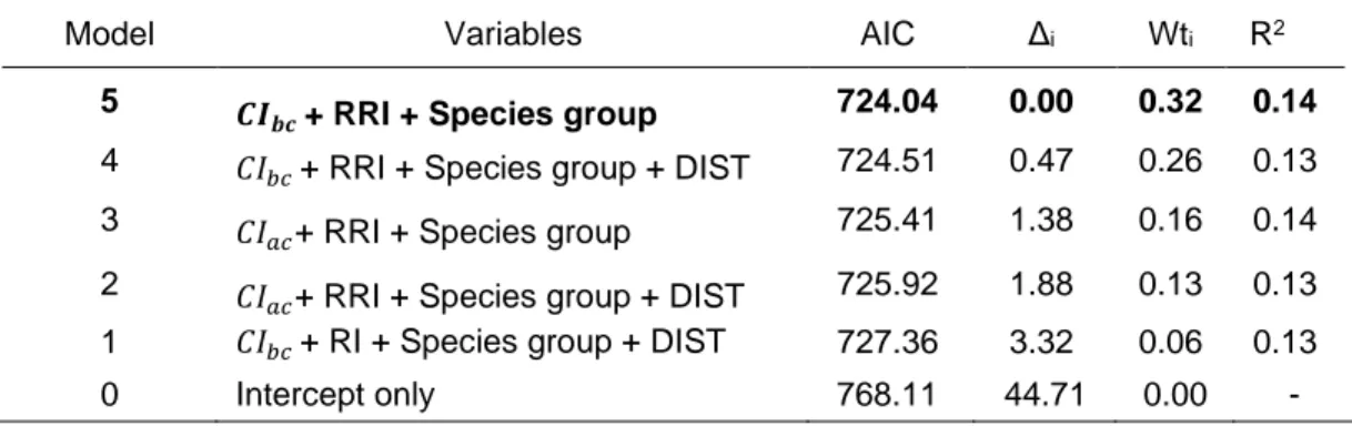
significant effect of RRI (p = 0.054), while the distance to the nearest skid trail (p = 0.50), the species group (p = 0.45) and the release index (p = 0.24) had clear non significant effects. The best model included 𝐶𝐼𝑏𝑐 and RRI as predictors (Table 1.3, model 5) with an

AIC weight of 0.60 and a conditional R2_{of 0.34. The addition of the RRI to the best model}

increased its parsimony but had only week effect on the R2. Multi-model inferences indicated that the unconditional confidence intervals of only one parameter (𝐶𝐼𝑏𝑐) excluded zero (Table

1.4). This result indicates that although RRI was part of the model with the lowest AIC, this variable did not contribute much to explain the variation in sugar maple growth. According to model 4, the tree growth response increased with decreasing competition before the cut (Fig. 1.2). An examination of the RRI values showed that 42 % of the trees in the database did not experience a release (RI and RRI value of 0), which implies that no change in competitive environment occurred in a 6-m radius after harvest.

Table 1.3 Model selection results for the five best regression models predicting the basal area growth response of trees during a 10-year period following selection cuts. 𝐵𝐴𝐼10 is the

mean annual basal area increment for the 10 years prior to cutting, 𝐶𝐼𝑎𝑐 is the competition

index computed immediately after selection cutting, 𝐶𝐼𝑏𝑐 is the competition index computed

immediately before selection cutting, DIST is the distance to nearest skid trail, RRI is the relative release index and RI is the release index. AIC is the Akaike Information Criteria, Δi is the delta AIC (difference in AIC with the best model), Wti is the AIC weight, R2

MR is the

marginal coefficient of correlation and R2

CN is the conditional coefficient of correlation. All

models included an intercept among the fixed effects as well as a plot-level random intercept.

Model Variables AIC Δi Wti R2MR R

2_CN 5 ln (𝑪𝑰𝒃𝒄) + RRI 198.71 0.00 0.37 0.27 0.34 4 ln (𝐶𝐼𝑏𝑐) 200.34 1.63 0.16 0.26 0.33 3 ln (𝐶𝐼𝑏𝑐) + RI 200.45 1.74 0.16 0.27 0.33 2 ln (𝐶𝐼𝑏𝑐) + RI + DIST 200.62 1.91 0.14 0.27 0.24 1 ln (𝐶𝐼𝑎𝑐) + RRI 202.22 3.51 0.06 0.26 0.32 0 Intercept only 284.05 85.35 0.03 - -