What causes the forecasting failure of Markov-switching models ? A Monte Carlo study

EURIsCO, Université Paris Dauphine

cahier n° 2003-10

par

Marie Bessec & Othman Bouabdallah

What causes the forecasting failure

WHAT CAUSES THE FORECASTING FAILURE OF

MARKOV-SWITCHING MODELS ? A MONTE CARLO

STUDY

Marie BESSEC

_{Othman BOUABDALLAH}

October 15, 2003

Abstract

This paper explores the forecasting abilities of Markov-Switching models. Although MS models generally display a superior in-sample fit relative to linear models, the gain in prediction remains small. We confirm this result using simulated data for a wide range of specifications. In order to explain this poor performance, we use a forecasting error decomposition. We identify four components and derive their analytical expressions in different MS specifications. The relative contribution of each source is assessed through Monte Carlo simulations. We find that the main source of error is due to the misclassification of future regimes.

Keywords: Forecasting, Regime Shifts, Markov Switching. JEL classifications: C22,C32,C53.

1

Introduction

Since the seminal paper of Hamilton (1989), there is a great deal of interest in modelling time series that are subject to structural changes using Markov-Switching (MS). The cyclical behaviour of many economic variables has been of particular interest.

Several recent studies use MS models to predict economic series (see for example Clements and Krolzig, 1998, Krolzig, 2003). However, the results are disappointing. Although MS models give a better in-sample fit relative to linear models, they are usually outperformed by linear models in out-of-sample forecasting exercises. Dacco and Satchell (1999) present a theoretical explanation for this bad performance in a fairly simple specification. They consider a model with

∗_{marie.bessec@dauphine.fr, EURISCO, University of Paris Dauphine.}

no autoregressive terms and with a switch on the intercept. They show that only a small mis-classification of future regimes, due to the failure to forecast the regime indicator, dramatically deteriorates the predictions of this model.

The aim of this paper is to assess the robustness of this result on a wide range of specifications. To this end, we perform a Monte Carlo study. First, the quality of the linear and non-linear predictions are compared. Second, the forecasting error is decomposed as suggested in Krolzig (2003). The analytical expressions of the four different sources of error are derived and their relative contribution is assessed using simulated data.

We focus on specifications with only a shift in the deterministic part where it is possible to derive analytically optimal predictors (Krolzig, 2003). We consider a wide range of specifications for these models. Representations with a switching intercept (and variance) or a switching mean (and variance) are studied using different sets of parameters1. In particular, we examine the impact of changes in the persistence and error-variance parameters. For all specifications, we show that the failure to predict the future regimes explains the major part of the total prediction error of the MS models.

The remainder of the paper proceeds as follows. Section 2 introduces the four subclasses of the models under study and reports the expression of the optimal predictor in these specifi-cations. Section 3 describes the simulation procedure and compares the performances of linear and non-linear models in forecasting exercises. Section 4 presents the error decomposition and discusses the simulation results that are based on it. Section 5 gives our concluding remarks.

2

Prediction in MS autoregressive models

Krolzig (2003) shows that analytical expressions for the optimal predictors can be derived in MS-VAR models only if the autoregressive parameters are time—invariant. For this reason, we have chosen to focus in the following sections on four important subclasses of MS-VAR models: specifications with switches only on the intercept (MSI), on the intercept and the variance (MSIH), on the mean (MSM) and on the mean and the variance (MSMH). As an illustrative example, we use the special case of univariate specifications with two regimes and one autoregressive term2_.

2.1

The MSI(H) Model

Let yt be the time series of interest. Suppose that yt follows a first autoregressive process

with a switch on the intercept (MSI). These switches occur between two states and are governed

1_{These specifications are widely used to capture the dynamics of real variables (Hamilton, 1989, Krolzig and}

Toro, 2002, Clements and Krolzig, 2003) and financial series (Cecchetti et al., 1990, Engel and Hamilton, 1990, Engel, 1994, Garcia and Perron, 1996, Bidarkota, 2001).

by an unobservable variable St which follows a first-order Markov process and takes the value 1

or 2.

yt= νst + αyt−1+ ut ut∼ NID(0, σ) (1)

Following Krolzig (2003), we can define an unobservable 2 × 1 state vector ξt consisting of

two binary indicator variables as ξ_t= [I(st= 1), I(st= 2)]0 and F the transition matrix of the

Markov process: F = µ p11 1 − p22 1 − p11 p22 ¶

The dynamics of the centered state vector of being in state one, ζ_t= ξ_{1t− ξ1}, is given by: ζ_t+1= (p11+ p22− 1)ζt+ vt+1 (2)

where ξ_{1 is the first component of the 2 ×1 vector of ergodic probabilities ξ = [P (s}t= 1), P (st=

2)]0 and vt is a martingale difference sequence.

The state space representation of this MSI(2)-AR(1) process can thus be defined by: ½

yt− µy = (ν1− ν2)ζt+ α(yt−1− µy) + ut

ζ_t+1= ρζ_t+ vt+1

(3) with ρ = p11+ p22− 1 and µy = (1 − α)−1(ν1, ν2) ξ.

It follows that the optimal predictor ˆy_t+h|t is given by:

ˆ y_{t+h|t− µy} = αh(yt− µy) + (ν1− ν2) Ã _h X i=1 αh−iρi ! ˆ ζ_t|t (4)

The second term in (4) represents the contribution of the non-linear part. The weight of this term increases with the shift on the intercept |ν1− ν2|, the persistence parameters α and ρ, and

diminishes with the horizon of prediction h. In the absence of change in the intercept (ν1 = ν2),

this equation reduces to the linear optimal predictor αh(yt− µy).

Note that this analytical expression also applies for a MSIH(2)-AR(1) process where the variance of ut depends on the state ut/st∼ NID(0, σst).

2.2

The MSM(H) Model

Let us now consider an AR(1) process with a switching mean as motivated by Hamilton (1989). The dynamics of a MSM(2)-AR(1) model is described by the following equation:

yt= µst + α(yt−1− µst−1) + ut ut∼ NID(0, σ) (5)

Using the same notations, the state space representation of this model is given by:    yt− µy = (µ1− µ2)ζt+ zt zt+1 = αzt+ ut+1 ζ_t+1= ρζ_t+ vt+1 (6)

with zt the autoregressive component of the process zt= yt− µst and µy = (µ1, µ2) ξ.

Using this representation, it is easy to show that the optimal predictor ˆy_t+h|t is obtained as follows: ˆ y_{t+h|t− µy} = αh(yt− µy) + (µ1− µ2) ³ ρh_{− α}h ´ ˆ ζ_t|t (7)

As above, the MSM predictor consists of two parts: the linear optimal predictor and a second part which takes into account the shifts in the mean. The weight of the last one depends on the magnitude of the shift |µ1− µ2| and on the persistence of the regimes ρ relative to the

persistence of the process α.

Again, this expression is still valid when we allow for a dependence of the variance on the realized regime st (MSMH(2)-AR(1) model).

3

Forecasting failure of MS models

Many studies show the poor performance of non-linear models against the linear counterpart for prediction. We explore the robustness of this result for a wide range of DGPs (MSI, MSIH, MSM and MSMH) and different sets of parameters.

To assess the relative performance of the two competing alternatives for forecasting purposes, we perform Monte Carlo simulations. We use the following procedure. First, data from one of the four MS processes are generated. Then, the linear and non-linear alternatives are estimated. Finally, the predictions are computed into the two models at different horizons h = 1, . . . , 8. The predictions are made in an out-of sample context with a rolling forecast origin and the estimated parameters are recalibrated at each iteration3. This procedure is replicated 1000 times. We consider samples with 200 observations4 and the forecast origin Tf rolls from 160 to 200 − h

for each horizon h. This exercise is repeated for different values of the transition probability p22∈ {0.70; 0.85} and of the variance parameter σ ∈ {0.3; 0.5}. The other parameters are chosen

close to the estimates of the Hamilton model of the US GNP growth rate (1989): µ₁ = ν1 = 1 ;

µ₂ = ν2 = −1 ; α = 0.2 ; p11= 0.95.

The results are summarized in Tables 1 and 2. We report the relative Mean Absolute Error (MAE) and Root Mean Square Error (RMSE) of the MS predictor to the linear one5. A result inferior to one indicates that the Markov Switching model performs better than the linear alternative and vice versa.

3

Note that this choice is consistent with Tashman (2000). He shows that the efficiency and reliability of out-of-sample tests can be improved by employing rolling-origin evaluations and recalibrating coefficients.

4

We remove the first 100 observations of the 300 observations initially generated, in order to avoid the possible effects of the initial conditions.

5

We have only reported the results for univariate specifications. However, our findings are still valid in the bivariate case. The corresponding results are available upon request.

Several findings emerge from the two tables. First, the gain of the non-linear alternative relative to the linear one is rather small, although the data are generated from a MS model. Indeed, the gain never exceeds 10% and shrinks to zero for large horizons (as shown above). Such a result is consistent with findings obtained in previous studies (Clements and Krolzig, 1998, Krolzig, 2003). Second, the comparison of the three DGPs shows that the MSIH displays an enhancement of no more than 10% (with the MAE criteria) at short horizons. At longer horizons, the MSM or MSMH specifications provide the best relative performance with a maximum gain of 6% (using the RMSE criteria). Third, for each DGP, increasing the variance parameter generally leads to a slight deterioration of the MS prediction. On the contrary, an increase in the persistence of the regimes improves the relative performance of the non-linear specification up to 6%. This increase also slows down the convergence of the non-linear predictor with the linear one as predicted by equations (4) and (7).

Table 1: Comparison of models with MAE

MSI MSIH MSM MSMH σ 0.3 0.5 0.3, 0.5 0.3 0.5 0.3, 0.5 p22 0.70 0.85 0.70 0.85 0.70 0.85 0.70 0.85 0.70 0.85 0.70 0.85 1 0.92 0.88 0.94 0.90 0.92 0.88 0.95 0.91 0.96 0.92 0.95 0.91 2 0.97 0.93 0.97 0.92 0.96 0.90 0.97 0.92 0.98 0.92 0.97 0.92 3 0.99 0.96 0.99 0.94 0.99 0.94 0.99 0.94 0.99 0.94 0.99 0.93 4 1 0.98 1 0.96 1 0.96 1 0.96 1 0.96 1 0.95 5 1 0.99 1 0.98 1 0.97 1 0.97 1 0.97 1 0.96 6 1 1 1 0.98 1 0.98 1 0.98 1 0.98 1 0.97 7 1 1 1 0.99 1 0.99 1 0.99 1 0.99 1 0.98 8 1 1 1 1 1 0.99 1 0.99 1 0.99 1 0.99

Table 2: Comparison of models with RMSE

MSI MSIH MSM MSMH σ 0.3 0.5 0.3, 0.5 0.3 0.5 0.3, 0.5 p22 0.70 0.85 0.70 0.85 0.70 0.85 0.70 0.85 0.70 0.85 0.70 0.85 1 0.96 0.94 0.96 0.93 0.95 0.93 0.98 0.93 0.98 0.95 0.98 0.95 2 0.98 0.97 0.98 0.95 0.98 0.95 0.99 0.94 0.99 0.96 0.99 0.96 3 1 0.98 0.99 0.97 0.99 0.97 1 0.96 1 0.97 0.99 0.97 4 1 0.99 1 0.98 1 0.98 0.99 0.97 1 0.98 1 0.98 5 1 0.99 1 0.99 1 0.99 1 0.98 1 0.99 1 0.99 6 1 1 1 1 1 0.99 1 0.99 1 0.99 1 0.99 7 1 1 1 1 1 1 1 0.99 1 0.99 1 0.99 8 1 1 1 1 1 1 1 1 1 1 1 1

4

Forecasting error decomposition

To explain such a poor performance of the MS specifications, we decompose the forecast error of the non-linear models into four components as suggested by Krolzig (2003).

The prediction error ˆe_t+h|t = yt+h− E[yt+h/ Ωt; bΘ] associated with the optimal predictor

b

y_t+h|t can be written as follows: ˆ e_t+h|t = (yt+h− E[yt+h/ st+h, Ωt; Θ0]) + (E[yt+h/ st+h, Ωt; Θ0] − E[yt+h/ st, Ωt; Θ0]) + (E[yt+h/ st, Ωt; Θ0] − E[yt+h/ Ωt; Θ0]) + (E[yt+h/ Ωt; Θ0] − E[yt+h/ Ωt; bΘ]) (8)

Θ0 is the set of actual parameters, ˆΘ the estimated set of parameters and Ωt the information

set available at time t. The first component ˆe(1)_t+h|t reflects the error we get if we know the exact set of parameters and the dynamics of the Hidden Markov process st+h= {st+h, st+h−1,...,st−1}.

This source of uncertainty reduces to the unpredictable Gaussian components (us)t<s≤t+h. The

second term ˆe(2)_t+h|t measures the contribution of the regime prediction error, i.e. the impact of the misclassification of future values of the Markov process. The third one ˆe(3)_t+h|t measures the error due to the filter uncertainty, that is the error induced by the filtering process of the past and current states involved in the prediction. These three components are evaluated conditional to the true parameters Θ0. The last component ˆe(4)_t+h|t stands for the parameter uncertainty due

to the estimation procedure6_.

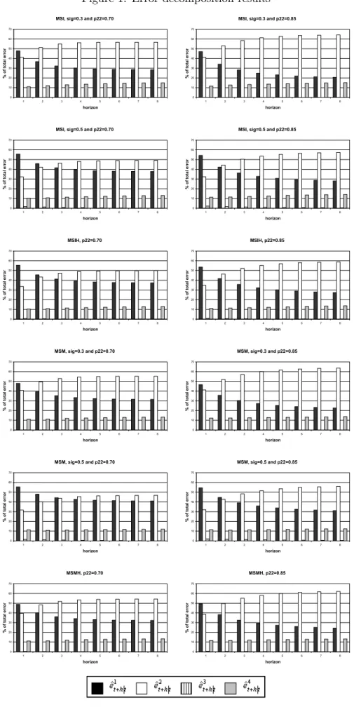
We apply this decomposition in the Monte Carlo design described above. For each DGP analyzed in Section 3, the relative weights of each component in absolute value for the eight horizons are depicted in Figure 1. Several results are worth commenting on. First, the third component ˆe(3)_t+h|t is found to be insignificant in all specifications and at all horizons. Second, the weight of the estimation error ˆe(4)_t+h|t remains stable and small over all specifications (10-14%). Hence, the two major sources of forecasting error are due to the Gaussian terms and the misclassification of future states. The relative part of these two terms varies across the horizon. The first component is the most important at the first horizon (h = 1). For larger h, the second component ˆe(2)_t+h|tdominates with a weight increasing with the horizon and ranging from 40% to 65%. Such a contribution is positively related to the persistence of the regime. On the contrary, it tends to decrease with the volatility. This last result is intuitive: a larger variance gives a heavier weight to the unpredictable component, ˆe(1)_t+h|t.

6

See the Appendix B for the derivation of each component in the MSI(m)-VAR(p) and MSM(m )-VAR(p) specifications.

5

Conclusion

In this paper, we have examined the performances of Markov-Switching models in predicting economic variables that are subject to regime switching.

A simulations-based study has shown that the improvement in the forecast performance is rather small compared to the linear specification and occurs only at short horizons. Checking the relevance of this result for different parameter settings has shown the robustness of this finding. Indeed, changing the persistence parameters and the variability of the process does not significantly affect the forecasting performance of the MS models relative to the linear one.

To explain this result, we have performed a forecasting error decomposition exercise. Four different sources of error have been identified and their relative contribution has been assessed using simulated data. It turns out that the misclassification of future-state realizations explains the failure of MS models in prediction exercises with an average contribution of 60% of the total error.

This result suggests that the prediction enhancements made in the MS models require im-proving the prediction of the states. This will be the subject of future research.

References

Bidarkota P.V. (2001), “Alternative Regime Switching Models for Forecasting Inflation”, Journal of Forecasting , 20(1), 21-35.

Cecchetti G.C., Lam P-S., Nelson C.M. (1990), “Mean Reversion in Equilibrium Asset Prices”, American Economic Review, 80(3), 398-418.

Clements M.P., Krolzig H.-M. (1998), “A Comparison of the Forecast Performance of Markov-Switching and Threshold Autoregressive Models of US GNP”, Econometrics Journal, 1, C47-C75.

Clements M.P., Krolzig H.-M. (2003), “Business Cycle Asymmetries: Characterization and Testing Based on Markov-Switching Autoregressions”, Journal of Business and Economic Sta-tistics, 21(1), 196-211.

Dacco R., Satchell C. (1999), “Why do Regime-Switching Forecast So Badly?”, Journal of Forecasting, 18, 1-16.

Engel C. (1994), “Can the Markov Switching Model Forecast Exchange Rates?”, Journal of International Economics, 36(1-2), 151-165.

Engel C., Hamilton J.D. (1990), “Long Swings in the Dollar: Are They in the Data and Do Markets Know it?”, American Economic Review, 80(4), 689-713.

Garcia R., Perron P. (1996), “An Analysis of the Real Interest Rate Under Regime Shifts”, Review of Economics and Statistics, 78(1), 111-125.

Hamilton J.D. (1989), “A New Approach to the Economic Analysis of Nonstationary Time Series and the Business Cycle”, Econometrica, 57, 357-384.

Krolzig H.-M. (2003), “Predicting Markov-Switching Vector Autoregressive Processes”, Forth-coming in the Journal of Forecasting.

Krolzig H.-M., Toro J. (2002), “Classical and Modern Business Cycle Measurement: the European Case”, Working Paper, Fundacion Centro de Estudios Andaluces, No. 2002/20.

Tashman L.J. (2000), “Out-of-sample Tests of Forecasting Accuracy: an Analysis and Re-view”, International Journal of Forecasting, 16, 437-450.

Figure 1. Error decomposition results

MSI, sig=0.3 and p22=0.70

0 10 20 30 40 50 60 70 1 2 3 4 5 6 7 8 horizon % of total error

MSI, sig=0.3 and p22=0.85

0 10 20 30 40 50 60 70 1 2 3 4 5 6 7 8 horizon % of total error

MSI, sig=0.5 and p22=0.70

0 10 20 30 40 50 60 70 1 2 3 4 5 6 7 8 horizon % of total error

MSI, sig=0.5 and p22=0.85

0 10 20 30 40 50 60 70 1 2 3 4 5 6 7 8 horizon % of total error MSIH, p22=0.70 0 10 20 30 40 50 60 70 1 2 3 4 5 6 7 8 horizon % of total error MSIH, p22=0.85 0 10 20 30 40 50 60 70 1 2 3 4 5 6 7 8 horizon % of total error MSM, sig=0.3 and p22=0.70 0 10 20 30 40 50 60 70 1 2 3 4 5 6 7 8 horizon % of total error MSM, sig=0.3 and p22=0.85 0 10 20 30 40 50 60 70 1 2 3 4 5 6 7 8 horizon % of total error MSM, sig=0.5 and p22=0.70 0 10 20 30 40 50 60 70 1 2 3 4 5 6 7 8 horizon % of total error MSM, sig=0.5 and p22=0.85 0 10 20 30 40 50 60 70 1 2 3 4 5 6 7 8 horizon % of total error MSMH, p22=0.70 0 10 20 30 40 50 60 70 1 2 3 4 5 6 7 8 horizon % of total error MSMH, p22=0.85 0 10 20 30 40 50 60 70 1 2 3 4 5 6 7 8 horizon % of total error

APPENDIX

A

Optimal predictors

A.1

MSI-VAR model

If the variance and autoregressive parameters of a MS-VAR model are regime-invariant Aj,st = Aj for j ∈ {1, ..., p}, there exists a linear state space representation. For a

MSIH(m)-VAR(p) model, this representation can be written as follows: ½

yt− µy= Mζt+ A1(yt−1− µy) + ... + Ap(yt−p− µy) + ut

ζ_{t+1= Fζt}+ vt+1

where µ_y = (IK − A1 − . . . − Ap)−1(ν1, · · · , νm) ξ is the unconditional mean of yt, M =

(ν1− νm, · · · , νm−1− νm) and F =    p1,1− pm,1 · · · pm−1,1− pm,1 .. . ... p_{1,m−1− pm,m−1 · · · pm−1,m−1− pm,m−1}    is a (m − 1) × (m − 1) matrix.

Let us consider the VAR(1) representation of the VAR(p) process. Denoting xtthe Kp × 1

vector defined as xt =

¡

xt xt−1 · · · xt−p+1

¢0 _{where x}

t is a K × 1 vector, the state space

representation can be rewritten as: ½ yt− ¯µ = Hζt+ A(yt−1− ¯µ) + ut ζ_{t+1= Fζt}+ vt+1 where A =      A1 ... Ap−1 Ap IK 0 · · · 0 . .. . .. .._. 0 IK 0    

is a Kp×Kp matrix, ¯µ = E(yt) and H = ¡

M 0 · · · 0 ¢0 is a Kp × (m − 1) matrix.

It follows that the optimal predictor ˆy_t+h|t is given by:

ˆ y_{t+h|t− µy} = à _h X i=1 JK,KpAh−iHFi ! ˆ ζ_t|t+ JK,KpAh(yt− ¯µ) with Jn,np = (In 0n· · · 0n) a n × np matrix.

A.2

MSM-VAR model

The state space representation of a MSM(m)-VAR(p) model is given by:    yt− µy = Mζt+ zt zt+1= Azt+ ut+1 ζ_{t+1= Fζt}+ vt+1

where µ_y = (µ_{1, · · · , µm}) ξ is the unconditional mean of yt, M = (µ1− µm, · · · , µm−1− µm) and

In a MSM(m)-VAR(p) process, the optimal predictor ˆy_t+h|t is given by: ˆ y_{t+h|t− µy} = JK,KpAh(yt− ¯µ)+ ³ MFhJ_{(m−1),(m−1)p− J}K,KpAhM ´ ˆ ζ t|t where M = Ip⊗ M .

B

Error Decomposition

B.1

MSI-VAR model

In a MSI(m)-VAR(p) model, the expression of the optimal predictor for the estimated set of parameters is given by:

ˆ y_t+h|t= ˆµ_y+ à _h X i=1 JK,KpAˆh−iH ˆˆF i ! ˆ ζ_t|t+ JK,KpAˆh ¡ yt− b¯µ ¢

where ˆθ denotes the estimate of the parameter θ. The total prediction error is given by:

ˆ e_t+h|t = yt+h− E ³ yt+h ¯ ¯ ¯Ωt; ˆΘ ´ = yt+h− ˆy_t+h|t

This error can be decomposed into four components: ˆ

e_t+h|t= ˆe1_t+h|t+ ˆe_t+h|t2 + ˆe3_t+h|t+ ˆe4_t+h|t • First component (measures the effect of the Gaussian error):

ˆ e1_t+h|t= yt+h− E (yt+h|st+h, . . . , st, Ωt; Θ0) = yt+h− ˆy_t+h|t1 with ˆy_t+h|t1 = µ_y+ h P i=1 JK,KpAh−iHζt+i+ JK,KpAh ¡ yt− ¯µ ¢ .

• Second component (measures the effect of future regime misclassifications): ˆ e2_t+h|t= E (yt+h|st+h, . . . , st, Ωt; Θ0) − E (yt+h|st, Ωt; Θ0) = ˆy1_t+h|t− ˆy2_t+h|t with ˆy_t+h|t2 = µ_y+ µ _h P i=1 JK,KpAh−iHFi ¶ ζ_t+ JK,KpAh ¡ yt− ¯µ ¢ . We then deduce: ˆ e2_t+h|t = h X i=1 JK,KpAh−iH ¡ ζ_{t+i− F}iζ_t¢

This component is proportional to the error made in predicting the future states¡ζ_{t+i− F}iζ_t¢, i = 1, . . . , h.

• Third component (due to the error in detecting the current regime): ˆ e3_t+h|t= E (yt+h|st, Ωt; Θ0) − E (yt+h|Ωt; Θ0) = ˆy_t+h|t2 − ˆy_t+h|t3 with ˆy_t+h|t3 = µ_y+ µ _h P i=1 JK,KpAh−iHFi ¶ ˆ ζ_t/t+ JK,KpAh ¡ yt− ¯µ ¢ . It follows that: ˆ e3_t+h|t= h X i=1 JK,KpAh−iHFi ³ ζ_{t− ˆζt/t}´ ˆ

e3_t+h|t is related to the filtering error ³

ζ_{t− ˆζt/t} ´

.

• Fourth component (error due to the estimation process): ˆ e4_t+h|t= E (yt+h|Ωt; Θ0) − E ³ yt+h ¯ ¯ ¯Ωt; ˆΘ ´ = ˆy3_{t+h|t− ˆ}y_t+h|t

B.2

MSM-VAR model

Now, the optimal predictor ˆy_t+h|t is given by: ˆ y_t+h|t= ˆµ_y+³_{M ˆ}ˆ_FhJ_{(m−1),(m−1)p− J}K,KpAˆhMˆ ´ ˆ ζ t|t+ JK,KpAˆ h¡_y t− b¯µ ¢ In the same way, we can decompose the forecast error into four components: • First component (the Gaussian error):

ˆ e1_t+h|t= yt+h− E ³ yt+h ¯ ¯ ¯st+h, . . . , st, Ωt; Θ0 ´ = yt+h− ˆy_t+h|t1 with ˆy_t+h|t1 = µ_{y + MJ(m−1),(m−1)p}ζ_{t+h − J}K,KpAhMζt + JK,KpAh ¡ yt− ¯µ ¢ and st = ¡ st st−1 · · · st−p+1 ¢0_.

• Second component (misclassification of future regimes): ˆ e2_t+h|t= E³yt+h ¯ ¯ ¯st+h, . . . , st, Ωt; Θ0 ´ − E¡yt+h ¯ ¯st, Ωt; Θ0 ¢ = ˆy_t+h|t1 _{− ˆ}y_t+h|t2 with ˆy_t+h|t2 = µ_{y+ (MF}hJ_{(m−1),(m−1)p− J}K,KpAhM)ζt+ JK,KpAh ¡ yt− ¯µ ¢ . It follows that: ˆ e2_{t+h|t= M}³ζ_{t+h− F}hζ_t´ • Third component (the filtering error):

ˆ e3_t+h|t= E¡yt+h ¯ ¯st, Ωt; Θ0 ¢ − E (yt+h|Ωt; Θ0) = ˆy_t+h|t2 − ˆy3_t+h|t with ˆy3 t+h|t= µy+ (MFhJ(m−1),(m−1)p− JK,KpAhM)ˆζt/t+ JK,KpAh ¡ yt− ¯µ ¢ .

We then deduce: ˆ

e3_{t+h|t= (MF}hJ_{(m−1),(m−1)p− J}K,KpAhM) (ζt− ˆζt/t)

Note that this error is now dependent on the filtering of the current as well as of the p-1 past regimes.

• Fourth component (due to the estimation error): ˆ e4_t+h|t= E (yt+h|Ωt; Θ0) − E ³ yt+h ¯ ¯ ¯Ωt; ˆΘ ´ = ˆy3_{t+h|t− ˆ}y_t+h|t