Smooth sigmoid wavelet shrinkage for non-parametric estimation
Texte intégral
Figure
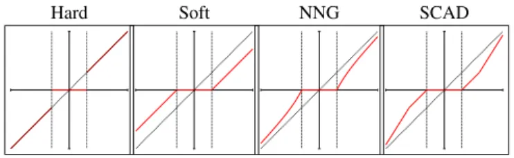
![Fig. 2. The SSBS functions δ τ , λ for different values of τ . It follows that τ parameterizes the curvature of the arc A 0O A , that is, the arc of the SSBS function in the interval ] − λ , λ [](https://thumb-eu.123doks.com/thumbv2/123doknet/12279711.322343/3.918.556.760.115.262/functions-different-values-follows-parameterizes-curvature-function-interval.webp)

Documents relatifs
The results obtained to the previous toy problem confirm that good performances can be achieved with various thresholding rules, and the choice between Soft or Hard thresholding
Block Coordinate Descent for Linear Regression For an arbitrary design matrix X, problem (20) can be solved using a Block Coordinate Descent (BCD) algorithm.. The main idea of the
The performance of these methods is an improvement upon other methods proposed in the literature and are algorithmically simple for large computational saving.. The proposed
In contrast to the “sum of derivative of Gaussian” parameterization of [13], the SSBS functions are defined by an explicit close form so that we can first adapt their shape according
The presentation of this work is as follows. Section 2 presents the SigShrink functions. Section 3 briefly describes the non-parametric estimation by wavelet shrinkage and addresses
Abstract — The classic example of a noisy sinusoidal signal permits for the first time to derive an error analysis for a new algebraic and non-asymptotic estimation technique..
Dans ce papier nous avons choisi les représentions de spectrogramme et de transformée en ondelettes pour ses propriétés spéciales et intéressantes, ces représentations
Block thresholding and sharp adaptive estimation in severely ill-posed inverse problems.. Wavelet based estimation of the derivatives of a density for m-dependent
