Capacity Results on Multiple-Input Single-Output Wireless Optical Channels

MIMO results presented above have been obtained with 50 sensors. We now assess the convergence of the MIMO estimates with increasing numbers of sensors distributed uniformly along

The zeolites are nano- or microsized porous inorganic crystals, which contain molecular sized regular channels (pores). Because of their unique pore size and shape, their

To save the power of each node and to limit the number of emission from the relay node, one solution is to aggregate small messages send by the end device?. To achieve this goal,

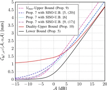
This paper studies the capacity of a general multiple-input multiple-output (MIMO) free-space optical intensity channel under a per-input-antenna peak-power constraint and a

It compares the numerically computed density, with the lower bound obtained in Theorem 1, and the lower bound obtained in [1] for ZF interference cancellation at the receiver for

Our formulae are Hobbs’s conjunctions of atomic predications, possibly involving FOL variables. Some of those variables will occur both in the LHS and the RHS of an I/O generator,

The proposed approach is based on the characterization of the class of initial state vectors and control input signals that make the outputs of different continuous

The elasto-capillary coiling mechanism allows to create composite threads that are highly extensible: as a large amount of fiber may be spooled inside a droplet, the total length X