HAL Id: hal-02749819
https://hal-imt-atlantique.archives-ouvertes.fr/hal-02749819
Submitted on 30 Nov 2020HAL is a multi-disciplinary open access
archive for the deposit and dissemination of sci-entific research documents, whether they are pub-lished or not. The documents may come from teaching and research institutions in France or abroad, or from public or private research centers.
L’archive ouverte pluridisciplinaire HAL, est destinée au dépôt et à la diffusion de documents scientifiques de niveau recherche, publiés ou non, émanant des établissements d’enseignement et de recherche français ou étrangers, des laboratoires publics ou privés.
Multilabel classification of remote sensed satellite
imagery
Ajay Kumar, Kumar Abhishek, Amit Kumar Singh, Pranav Nerurkar,
Madhav Chandane, Sunil Bhirud, Dhiren Patel, Yann Busnel
To cite this version:
Ajay Kumar, Kumar Abhishek, Amit Kumar Singh, Pranav Nerurkar, Madhav Chandane, et al.. Mul-tilabel classification of remote sensed satellite imagery. Transactions on emerging telecommunications technologies, Wiley-Blackwell, 2020, pp.e3988. �10.1002/ett.3988�. �hal-02749819�
DOI: xxx/xxxx
PREPRINT TO TRANSACTIONS ON EMERGING TELECOMMUNICATIONS TECHNOLOGIES
Multi-label Classification of Remote Sensed Satellite Imagery
†
Ajay Kumar*
1| Kumar Abhishek
1| Amit Kumar Singh
1| Pranav Nerurkar
2,3| Madhav
Chandane
2| Sunil Bhirud
2| Dhiren Patel
2| Yann Busnel
41Dept. of CSE, NIT Patna, Bihar, India 2Dept. of CE & IT, VJTI Mumbai,
Maharashtra, India
3Dept. of Data Science, MPSTME, NMIMS,
Mumbai, Maharashtra, India
4SRCD department, IMT Atlantique, IRISA,
Rennes, France
Correspondence
*Ajay Kumar, Dept. of CSE, NIT Patna. Email: [email protected]
Present Address
Dept. of CSE, NIT Patna, Bihar, India
Abstract
Multi-label scene classification has emerged as a critical research area in the domain of remote sensing. Contemporary classification models primarily emphasis on a sin-gle object or multi-object scene classification of satellite remote sensed images. These classification models rely on feature engineering from images, deep learn-ing, or transfer learning. Comparatively, multi-label scene classification of V.H.R. images is a fairly unexplored domain of research. Models trained for single label scene classification are unsuitable for the application of recognizing multiple objects in a single remotely sensed V.H.R. satellite image. To overcome this research gap, the current inquiry proposes to fine-tune the state of the art Convolutional Neural Network (C.N.N.) architectures for multi-label scene classification. The proposed approach pre trains C.N.N on the ImageNet dataset and further fine-tunes them to the task of detecting multiple objects in V.H.R. images. To understand the efficacy of this approach, the final models are applied on a V.H.R. dataset: the U.C.M.E.R.C.E.D. image dataset containing twenty-one different terrestrial land use categories with a sub-meter resolution. The performance of the final models is compared with Graph convolutional network-based model by N Khan et al.. From the results on perfor-mance metrics, it was observed that proposed models achieve comparable results in significantly fewer epochs.
KEYWORDS:
Remote sensing; Converged and future applications; Aerial imagery; Satellite image processing; Deep learning
1
INTRODUCTION
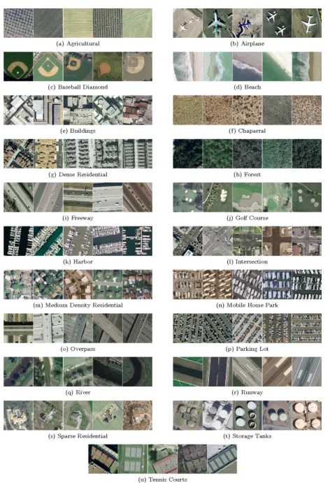
Land Use (L.U.) classification from remote sensed terrestrial imagery obtained using satellites is critical for monitoring and managing human-made activities1,2. This is not possible for processing using manual methods due to the voluminous amount of data that is generated from satellite images3. Besides, automated classification via machine learning is critical for understanding the constantly changing the surface of the earth, especially anthropomorphic changes4,5. However, the classification of terrestrial imagery is a momentous challenge because the terrain that symbolizes a given type of land use may have variability, and a few identical objects are shared among different terrain categories6. Figure 1 gives the 5 sample images present in each of the 21
†Remote sensing with deep learning.
0Abbreviations: V.H.R., Very high resolution; U.C., University of California; BoVW, Bag of visual words
0Authorship: All authors contributed equally towards the design of the work, data analysis and interpretation, drafting, and critical revision of the article. A. Kumar
A Kumar
classes of U.C.M.E.R.C.E.D. land-use dataset7. Each of the five sample images belong to a particular category yet have large variability in appearance.
FIGURE 1 U.C.M.E.R.C.E.D. land use dataset contains 100 images from 21 land-use classes
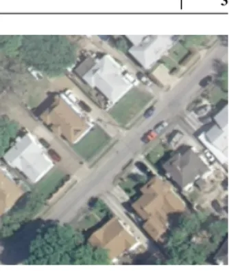
Due to the high variability in the composition of the terrain and the voluminous amount of terrain categories, optimal identi-fication with labeling for terrain types in V.H.R. Data have become challenging to solve using machine learning methods8,9,10. This challenge has ignited interest in the domain of remote sensing11,6. Additionally, terrestrial images obtained from satellites or aerial objects of land use contain several objects within the same image. In Figure 2 a, the label associated with the image is
𝐴𝑖𝑟𝑝𝑜𝑟𝑡, Figure 2 b belongs to label 𝐵𝑎𝑠𝑒𝑏𝑎𝑙𝑙𝑑𝑖𝑎𝑚𝑜𝑛𝑑 and Figure 2 c belongs to label 𝑀 𝑒𝑑𝑖𝑢𝑚𝑟𝑒𝑠𝑖𝑑𝑒𝑛𝑡𝑖𝑎𝑙. Each image has multiple objects present within it, as indicated in the corresponding caption.
To effectively and efficiently label terrain types from satellite images, the literature proposes several techniques. State of the art techniques focus on deep neural architectures, which learn tiered inner feature embeddings from visuals datasets and create near-human performance. Nevertheless, a majority of approaches, counting even the conservative vanilla neural network
(a) airplane, cars, grass and pavement (b) bare soil, building, grass, pavement (c) cars, pavement, grass, trees, bare soil, building
FIGURE 2 U.C.M.E.R.C.E.D. dataset images consisting of multiple objects
methods and deep neural networks, solitarily focus on fitting a model to recognize a single label within an image12. Multi-label classification of very high resolution (V.H.R.) images is still to receive sufficient attention in the scientific literature13.
Analyzing the timeline of the automated labeling of terrain in V.H.R. reveals a broad spectrum of techniques. Traditional image feature extraction (F.E.) and image processing techniques used handcrafted FE4that relied on kernels to extract features. The mainstream conventional frameworks, such as the bag-of-visual words (BoVW) centered terrain extract cataloging technique, rely on heuristics that measure features such as color histogram, local binary pattern, and scale-invariant feature transform (S.I.F.T.) among others in a visual and allot a semantic identifier to the visual according to its essence12. Although F Zhang et al. argue that the BoVW approach achieves the state of the art efficiency, its ability to tackle complex terrestrial images of land use is constrained as it fails to encompass spatial and structural information in the V.H.R. image11,6. Though FE and BoVW methods have achieved excellent performance, despite relying on low-level image features obtained through kernels. The inadequate expressive capability of these primitive and intermediate level hand-engineered features has become a bottleneck for improving their LU scene classification performance14. The main drawback of F.E. and BoVW based techniques lies in the assumption that a general feature descriptor can adequately represent the complex image structures by employing expert knowledge through manually designed all-around purpose features13.
The maximum contemporary effort in visual classification has been concentrated on Deep-learning (D.L.) algorithms that employ unsupervised learning of adequate and discriminative feature representations from unlabelled input data11as shown in Figure 3 .
FIGURE 3 Deep learning models for satellite image processing
Deep-learning (D.L.) algorithms, which learn complex and nonlinear representative and discriminative features in a tiered manner from the inputs, are an emerging field in the artificial intelligence community and have entered into the satellite image processing community for R.S. unstructured data analysis15,16,17. This new field of investigation opened by deep learning has led to mushrooming of literature and frameworks4,12. As D.L. algorithms are computationally expensive and time-consuming to train, transfer learning approach was utilized to overcome these issues. In transfer learning, knowledge learned from training the model on a particular dataset is transferred to a different problem. This approach enables the training of D.L. models on tasks where data is limited.
A Kumar
The critical contribution of the current paper is proposing a deep learning-based convolutional neural network model for the multi-label scene classification of V.H.R. images. To overcome the issue of model overfitting due to limited data availability, fine-tuning is used. To elaborate on fine-fine-tuning, initially, the C.N.N. models are pre-trained on the ImageNet dataset, and additional layers are added to the models. The additional layers are trained on the dataset for the task of recognizing multiple objects in images. In spite of extensive literature review, multi-label classification of U.C.M.E.R.C.E.D. Land Use V.H.R. Images using pre-trained D.L. models was not found. Hence, the contribution extends the research in this domain. For the experimental study, 16 selected deep learning architectures pre-trained on the ImageNet dataset were fine-tuned and applied on the multi-label classification of U.C.M.E.R.C.E.D. L.U. Dataset on standard parameters, a discussion is presented along-with the conclusion and future course of action.
The contents in the current research are grouped as follows. In Section 2, a brief review of the related works about fea-ture engineering based classifiers, unsupervised feafea-ture engineering based classifiers, and transfer learning-based classifiers are introduced. In Section 3, the pre-trained D.L. models are described in detail. The details of the experiments and the results are presented in Section 4. Eventually, Section 6 draws the outcome of this paper with an elaboration of the results and guidelines for future work.
2
REVIEW OF LITERATURE
The current endeavors in the literature can be grouped into three categories: techniques based on handcrafted features, techniques based on data-driven features, and techniques based on transfer learning (see Figure 4 ). The review describes the methodologies used by techniques in each category. It is concluded from the literature, that multi-label classification on V.H.R. images has not received sufficient attention.
FIGURE 4 Categories of machine learning models for land use classification
2.1
Feature engineering-based classifiers
E Aptoula18 focused on Content-based image retrieval (C.B.I.R.) using global image descriptors. The author speculated that global image descriptors are more efficacious in C.B.I.R. compared to local descriptors. Results of applying global morpholog-ical texture descriptors (circular covariance histogram (C.C.H.), rotation-invariant point triplets (R.I.T.), and descriptors based on Fourier power spectrum of the quasi-flat-zone-based scale space (F.P.S.)) on U.C.M.E.R.C.E.D. land-use (U.M.L.U.) dataset are presented. The author has concluded through experimentation that features of the image extracted using C.C.H., R.I.T. and F.P.S. is more suitable for C.B.I.R. compared to local descriptors on the U.M.L.U. dataset7. L Gueguen19proposed a compound structure representation for image classification. It utilized local features descriptors extracted from the multiscale segmentation of the original image. The extracted features are clustered into visual words with the KD-Tree algorithm. Distributions of the visual words are used to elaborate on the image compound structures. N He20proposed a framework to combine two low-level visual features viz. Gabor feature and color feature for scene classification. S Kumar et al.21proposed a parallel architecture for extraction of morphological features such as circular covariance histogram (C.C.H.), rotation-invariant point triplets (R.I.T.).
2.2
Unsupervised feature engineering based classifiers
J Fan et al.22argued that handcrafted feature descriptors (local and global) are less suitable for image recognition compared to features learned from the image data in a data-driven manner. The authors have preferred an unsupervised learning approach for learning feature descriptors from images using multi-path sparse coding architecture. F Luus et al.23use a deep convolutional layer neural network (D.C.N.N.) for image classification. The authors prefer to avoid handcrafted features relying instead on D.C.N.N. for feature determination. R Stivaktakis et al.24proposed a multi-label image classification architecture using D.C.N.N. To avoid model overfitting, data augmentation techniques such as rotation of the visual by various degrees, image re-scaling, horizontal and vertical flips, translations to the x and y-axis, and the incorporation of noise were used. H Wu et al.14proposed a hybrid architecture called deep filter banks. It combined multicolumn stacked denoising sparse autoencoder (S.D.S.A.E.) and Fisher vector (F.V.) to consequently infer the complex nonlinear features in a hierarchical manner for L.U. Scene classification in the U.M.L.U. Dataset. F Zhang et al.11 proposed an unsupervised feature learning framework using the saliency detection algorithm to extract an illustrative set of areas from the significant regions in the U.M.L.U. Image dataset. These representative patches were given as input to a sparse auto-encoder to convert these image patches into low-dimension feature vectors. The training of the S.V.M. was performed using these feature vectors for image classification.
F Zhang et al.12proposed a gradient boosting random convolutional network (G.B.R.C.N.) framework for scene classification. It was an ensemble framework consisting of multiple single deep neural networks. J Bergado et al.25proposed a multi-resolution convolutional network, called FuseNet, and its recurrent version, called ReuseNet, to perform image fusion, classification, and map regularization of a multi-resolution V.H.R. image in an end-to-end fashion. Z Gong et al.26 introduces structured metric learning, a strategy that modifies the binary cross-entropy loss metric to allow it to discriminate the remote sensing image scenes with the great similarity. The new metric is incorporated into a D.C.N.N. model for image classification in U.M.L.U. Dataset. C Cao et al.27 concentrated on the estimation of eight transferred C.N.N.-based models on land-use classification tasks and submission of the optimal performing transferred C.N.N.-based model as a discriminator to classify and plot the land-use.
R Minetto et al.28proposed Hydra, an ensemble of convolutional neural networks (C.N.N.) for geospatial land classification. The ensemble of C.N.N. is created from ResNet and DenseNet architectures pre-trained on the ImageNet dataset. Additional layers of ResNet and DenseNet architectures are added to create an end-to-end deep learning pipeline for image classification. H Parmar29 proposed a multi-neighborhood LBPs combined with the nearest neighbor classifier that can achieve an accuracy of 77.76% for image classification on U.M.L.U. Dataset. In30, K Karalas et al. utilize a C.N.N. to categorize the dissimilar types of terrestrial covers by allocating one or more labels to perceived spectral vectors of the multi-spectral image pixels.
2.3
Transfer learning approach for classification
D Marmanis et al.13extended the use of D.C.N.N. in image classification by utilizing a DCNN pre-trained on ImageNet dataset instead of training a DCNN from scratch. The authors argued that the large pre-trained deep convolutional neural network (D.C.N.N.) generated a set of high-level representations, which could be used for image classification in the next processing stage. G Scott et al.4preferred features learned by D.C.N.N. from the training data than handcrafted features. The authors experimented with three architecture viz. CaffeNet, GoogLeNet, and ResNet50 for image classification on U.M.L.U. dataset. To improve the model performance, transfer learning and data augmentation were used. Q Weng et al.6used pre-trained C.N.N. to learn deep and robust features from the images of the U.M.L.U. Dataset. The authors modified the CNN architecture by replacing the fully-connected layers of the C.N.N. by the extreme learning machine classifier. Y Zhen et al.31also argued in favor of pre-trained deep neural networks for image classification. The authors modified the standard GoogLeNet with a structure called ’Inception’. The modified network reduced the parameters and trained faster compared to the original network. E Flores et al.32 used a ResNet-50 DCNN architecture pre-trained on the ImageNet dataset for feature extraction from images. The learned parameters of the ResNet-50 were used to extract 2048 bit deep feature vectors of each input image. These feature vectors were then used to classify the image. N Uba33utilized architectures of AlexNet, CaffeNet, and GoogleNet on ImageNet dataset and transferred the leanings of the model from the ImageNet dataset to the U.M.L.U. Dataset for image classification. M Castelluccio et al.34 speculated that training CaffeNet and GoogLeNet from scratch would not be advisable for the limited-sized U.C.M.E.R.C.E.D. land-use (U.M.L.U.) dataset. The authors observed that careful fine-tuning of the CaffeNet and GoogLeNet architectures pre-trained on the ImageNet dataset, involving several layers of the architecture, provided good results, in general. J Li et al.35utilized a class activation map (C.A.M.) encoded C.N.N. model trained using original R.G.B. patches of ImageNet dataset and attention map based class information. The parameters of the architecture are then used for classification on the (U.M.L.U.) dataset.
A Kumar
Multi-label classification of U.M.L.U. Dataset is considerably more instinctive in remote sensing tasks. Considering the lack of research on pre-trained D.L. architectures in this domain, the scope of this work was defined. D.L. architectures were selected based on their accuracy (Top-1 and Top-5) on ImageNet35. Results obtained by these D.L. models were on a fixed experimental environment and hyper-parameters. Optimization of hyper-parameters or selecting the best D.L. model for the task is beyond the scope of this work.
3
DEEP LEARNING FRAMEWORKS
• V.G.G. proposed by K Simonyan et al. is a 3x3 stacked convolutional layer. It uses Max Pooling and Fully connected Networks, followed by Softmax classifier. It can be both 16 and 19 layered36.
• ResNet (or Residual Network) was first introduced by He et al. to solve the problem of gradient decay in deep neural network architectures through "shortcuts" in the network. These shortcuts are additive identity transformations of the previous nodes. It relies on micro-architecture modules referred to as "building blocks"37.
• C Szegedy et al. proposed InceptionNet which acts as a "multi-level feature extractor". It computes 1x1, 3x3 and 5x5 convolutions inside the same module of the network. It returns a stacked output along the channel dimension. Its weights are mere 96 MB, much smaller than VGG and ResNet38.
• Proposed by F Chollet, Xception is implemented in 2 steps, Spacial Dimension Transformation and Channel Dimension Transformation. In InceptionV3, a 1x1 convolution is followed by a 3x3 convolution allowing channels to merge first. While in Xception, the 3x3 space convolution takes place before the 1x1 channel convolution. It also has no Re.L.U. operation present in the architecture39.
• MobileNet is an application of Xception. When Xception attempts to improve accuracy, MobileNet is employed for both compressing the model and ensuring accuracy. A standard convolution is decomposed into depthwise and pointwise convolutions to reduce space40.
• DenseNet architecture attempts at improving Resnet architecture through gradient flow, improved parameter efficiency, and low complexity features. It achieves these by connecting each layer to every other layer in a feed-forward fashion. Hence, instead of L layers having L connections, DenseNet has L(L+1)/2 connections41.
TABLE 1 Models for visual classification mentioned with parameters trained on ImageNet39
Name Size in MB Top-1 Accuracy Top-5 Accuracy Parameters Depth
Xception 88 0.79 0.95 22,910,480 126 VGG16 528 0.71 0.90 138,357,544 23 VGG19 549 0.71 0.90 143,667,240 26 ResNet50 98 0.75 0.92 25,636,712 -ResNet101 171 0.76 0.93 44,707,176 -ResNet152 232 0.77 0.93 60,419,944 -ResNet50V2 98 0.76 0.93 25,613,800 -ResNet101V2 171 0.77 0.94 44,675,560 -InceptionV3 92 0.78 0.94 23,851,784 159 InceptionResNet 215 0.80 0.95 55,873,736 572 MobileNet 16 0.70 0.89 4,253,864 88 MobileNetV2 14 0.71 0.90 3,538,984 88 DenseNet121 33 0.75 0.92 8,062,504 121 DenseNet169 57 0.76 0.93 14,307,880 169 DenseNet201 80 0.77 0.94 20,242,984 201
Table 1 , shows results obtained by D.L. architectures on ImageNet. Top-1 and top-5 accuracy of the model are recorded based on its performance on the ImageNet validation dataset. Depth includes activation layers and batch normalization layers.
4
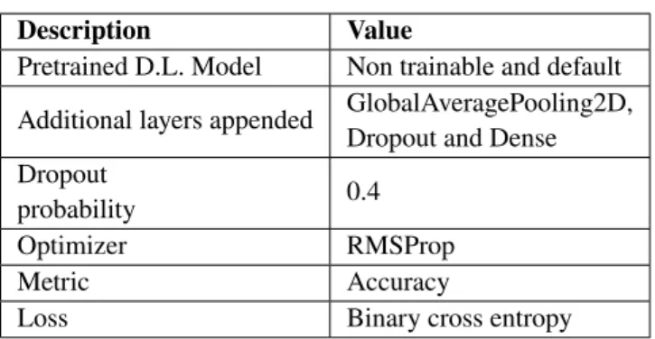
EXPERIMENTAL STUDY
Configuration of the system on which an experimental study was conducted had Windows7 OS with Intel(R) Core(T.M.) i5-6402P [email protected] with quad cores and 8GB DDR3 RAM. Implementations of the pre-trained D.L. models and default settings used were in Keras package using python39.
TABLE 2 Hyper-parameters of the models
Description Value
Pretrained D.L. Model Non trainable and default Additional layers appended GlobalAveragePooling2D,
Dropout and Dense Dropout
probability 0.4
Optimizer RMSProp
Metric Accuracy
Loss Binary cross entropy
Performance measures used for quantitative analysis are 𝐹1-score (Macro and samples), Precision (Macro and samples), Recall (Macro and samples), Number of parameters (Trainable, Non-Trainable and Total) and Threshold. The hyper-parameters of the models mentioned in Table 2 were fixed in order to reduce the degree of freedom in comparison.
4.1
Dataset
U.C.M.E.R.C.E.D. Land Use dataset7is a manually labeled ground truth dataset which consists of visuals of 21 terrain classes chosen from aerial orthoimagery with a sub-meter resolution. Each image is in the R.G.B. colorspace fetched from United States Geological Survey (U.S.G.S.) National Map. One hundred visuals measuring 256ÃŮ256 pixels are present for each of the 21 labels given in Table 3 (of Figure 1 ). Each image of the 21 classes contains multiple objects within it, as given in Table 3 .
5
RESULTS AND DISCUSSION
5.1
Analysis of precision and recall (macro and samples)
The results for the classification were analyzed using 𝐹1-score, Precision, and Recall. For the same, a confusion matrix is first made to get an overview of the results. A confusion matrix describes the performance of the classification model on the test data in a tabular form. Hence a summary of the prediction scores is obtained. The count of correct and incorrect predictions by each class is given, hence conveying the ways in which the classification model is confused while predicting.
Precision gives the percentage of positive results predicted correctly out of all the predictions made. Thus, a high precision value indicates that the positively predicted label is indeed positive. It can be thought of as the ability of a classification model to identify only the relevant data points.
𝑃 𝑟𝑒𝑐𝑖𝑠𝑖𝑜𝑛= 𝑇 .𝑃 .
𝑇 .𝑃 .+ 𝐹 .𝑃 .
This is a class level metric. To get an overall Precision or Macro Precision, we average out the class Precision.
𝑀 𝑎𝑐𝑟𝑜− 𝑃 𝑟𝑒𝑐𝑖𝑠𝑖𝑜𝑛 = 𝑃 𝑟𝑒𝑐𝑖𝑠𝑖𝑜𝑛1+ 𝑃 𝑟𝑒𝑐𝑖𝑠𝑖𝑜𝑛2
A Kumar
TABLE 3 The terrain types and their associated objects42
Terrain type Objects
agricultural field, trees
airport/airplane airplane, pavement, grass, building, car baseball diamond bare soil, pavement, grass, tree, building beach sea, sand, tree
urban area/buildings buildings, pavement, cars chaparral sand, chaparral
dense residential buildings, pavement, trees, cars forest trees, bare soil
freeway pavement, cars, grass, trees, bare soil golf course grass, trees, bare soil
harbor ship, dock, water
intersection pavement, bare soil, cars, building, grass medium residential buildings, cars, trees, grass, pavement, bare soil mobile home park mobile home, cars, pavement, trees, bare soil overpass pavement, cars, bare, soil, grass, trees parking lot cars, pavement, bare soil, grass river water, trees, bare soil
runway area/runway pavement, grass, bare soil
sparse residential buildings, grass, bare soil, tress, sand, chaparral storage tanks tanks, bare soil, grass, pavement, buildings tennis area/tennis court court, grass, trees, pavement, buildings
As Figure 5 suggests, Precision for ResNetV2- 50 was the highest at 0.918808 second only to ResNetV2- 101 by 2.25%. What is intriguing is that the least Precision is from the earlier versions of ResNet- ResNet50, ResNet101, and ResNet152 by 78.79%, 79.07%, and 80.67%. To understand the stark difference between the ResNets, we need to understand its origins37. ResNet was not the first to use the shortcut connection to overcome the gradient decay issue. Highway Networks had gated shortcut connections that controlled information flow across the shortcut. Hence ResNet, in many ways, is a special case of Highway Network. Strangely enough, while ResNet can be thought of as a subset of Highway Network, they tend to outperform them. Thus, the need to keep the gradient highways clear and restrain from going for a larger solution space is necessary. Hence the original ResNet was refined, and a pre-activation variant was proposed called ResNetV2. Gradients flow more freely through the shortcut connections. Hence, ResNet50V2 has 78.9% higher precision than ResNet50 in Figure 5 . Both ResNet50V2 and ResNet101V2 outperform VGG16 and VGG19 by 15.8% on an average. This could be attributed to deeper layers and a lack of gradient decay in ResnetV2.
InceptionV3 has a multi-modal architecture for predicting both globals through its 5x5 convolution layer and more salient features through its 1x1 convolution layer. It outperforms VGG16 and VGG19 by 10.61% and 5.83%, respectively. However, it could be a victim of gradient decay. Hence InceptionResnetV2, which is the combination of ResNet and InceptionV3, out-performs it by 1.9%. However, it is not better in predicting the True Positives from the positive predictions when compared to ResNet50V2 and ResNet101V2. It is less by 5.67% and 3.5%.
Xception is the modified Depthwise Separable Convolution. Its architecture is inspired by InceptionV3, with pointwise convolution taking place before depthwise convolution. It gives a better result than InceptionResnetV2 by 1.33%. However, ResNet101V2 still outperforms it by 4.4%. MobilenNet is lightweight in architecture and was developed on the lines of Xcep-tion. Its performance in terms of accuracy is not better than XcepXcep-tion. MobileNet has a Macro Precision of 0.813837, which is 7.34% less than Xception. In DenseNet121 and DenseNet169, has fully connected layers in a feed-forward way. Hence the num-ber of layers is L(L+1)/2 compared to convolutional networks with L layers. It is an advanced version of ResNet. However, the accuracy of DenseNet121 is 35.33% lower, and that of DenseNet169 is 11.47% lower than the Macro Precision of ResNet50V2. Clearly, the depth of the layer is not an issue here. This can be attributed to the long training time and memory requirement of DenseNet121 and DenseNet169.
FIGURE 6 Comparison between pretrained D.L. multi-label classifiers on Precision (samples)
A Kumar
From the figure, it is clear that the Macro Precision and Samples Precision are close to each other. For both the least values lie in ResNet50, ResNet101 and ResNet152. The highest Precision Samples are for VGG19, just 0.84% more than ResNet50V2, which is only 1.37% higher than ResNet101V2. MobileNet’s Precision Sample is higher than it is Macro Precision quite significantly, by 2.77%. The Precision Sample is higher than that of MobileNetV2 by 22.6% and interestingly more than the Xception network as well by 2.99%. All DenseNet values are less than those of ResNetV2 and more than ResNet.
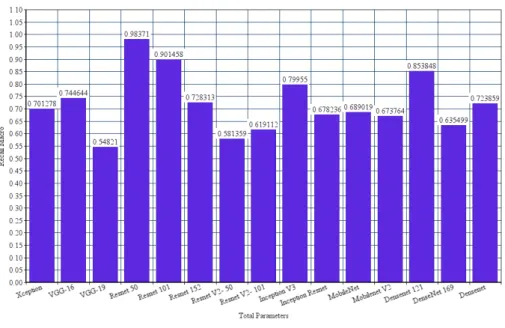
FIGURE 7 Comparison between pretrained D.L. multi-label classifiers on Recall (Macro)
Recall gives the percentage of positive results predicted correctly from all the actual positive results. It is regarded as a model’s ability to find all the data points of interest.
𝑅𝑒𝑐𝑎𝑙𝑙= 𝑇 .𝑃 .
𝑇 .𝑃 .+ 𝐹 .𝑁. The recall is also a class level metric. The overall Recall or the macro recall
is:-𝑀 𝑎𝑐𝑟𝑜− 𝑅𝑒𝑐𝑎𝑙𝑙 = 𝑅𝑒𝑐𝑎𝑙𝑙1+ 𝑅𝑒𝑐𝑎𝑙𝑙2
2
There tends to be a trade-off between Precision and Recall. The two differ only by one term in the denominator. For a given accuracy. if FP is high, FN is lower, meaning a lower Precision and higher Recall and vice-versa.
As visible from the Figure 7 , ResNet50 and ResNet101, and ResNet152, which had the lowest Macro Precision at 0.194986, 0.192298, and 0.177623, have an improved Recall of 0.98371, 0.0.90145 and 0.728313 respectively. Hence, we can conclude that the False Positives for ResNet is higher than the False Negatives. ResNet50 and ResNet101 have values higher than VGG16 and VGG19 on an average by 31.42%. ResNet50V2 and ResNet101V2 have Recall Macro value as 0.581359 and 0.619112, lower than their ResNet counterparts by 40.9% and 31.32% respectively. The Macro-Precision value for them was 0.918808 and 0.898132, hence a reduction by 36.72% and 31.06%, respectively. Hence for a given accuracy of ResNetV2, it can be said that the FN is higher than the FP. Recall Macro for InceptionV3 is higher than InceptionResNetV2 along with both ResNet50V2 and ResNet101V2 by 15.17%, 28.29% and 22.56% respectively. This was not true for Macro Precision, and hence it can be concluded that FP for InceptionV3 is higher than FN when compared to the above three models. The same is less by 18.72% and 11.30%, from ResNet50 and ResNet101, hence indicating a lower FP and a higher FN. As mentioned previously, Xception and MobileNet have similar architectures and hence are comparable. Xception has a higher Macro Recall value from MobileNet
and MobileNetV2 by 3.28% and 3.92%. However, the Macro Recall for Xception, MobileNet, and MobileNetV2 is lower than their Macro Precision value by 20.16%, 16.66%, and 6.44% respectively. Hence the FN values for the same are higher than FP. For Macro Recall, the values seem to reduce as more layers are added. ResNet50 has higher Macro Recall than ResNet101 by 8.36%, which in turn has higher Macro Recall than ResNet152 by 19.2%. Similarly, for VGG16/19, Macro Recall reduces by 26.38%. This is against the popular belief that more layers tend to increase accuracy, especially when it comes to ResNet, where gradient decay is being prevented up to some extent by design.
FIGURE 8 Comparison between pretrained D.L. multi-label classifiers on Recall (samples)
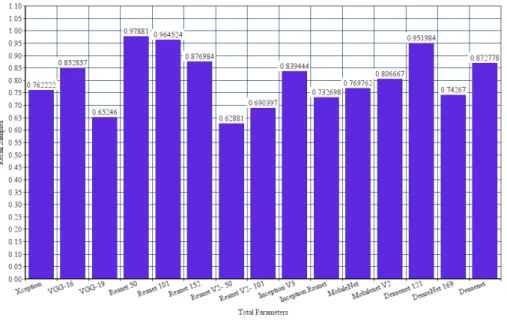
The highest Recall Samples continues to be that of ResNet50 (see Figure 8 ) with value peaking at 0.97881, slightly higher than ResNet101 by 1.46%. ResNetV2 continues being the worst performer for Recall, with ResNet50V2 having a Recall Sample 35.75% lesser than that of ResNet50. Recall Samples for DenseNet has improved overall. DenseNet121 has increased by 10.3%, only 2.74% lesser than ResNet50 compared to being 13.19% lesser for Macro Recall. The metric for VGG16 has increased by 12.68%.
5.2
Analysis of Macro 𝐹
1and 𝐹
1samples
𝐹1-score is the Harmonic Mean of Precision and Recall.
𝐹1= 2 ∗ 𝑃 𝑟𝑒𝑐𝑖𝑠𝑖𝑜𝑛∗ 𝑅𝑒𝑐𝑎𝑙𝑙
𝑃 𝑟𝑒𝑐𝑖𝑠𝑖𝑜𝑛+ 𝑅𝑒𝑐𝑎𝑙𝑙
The harmonic mean punishes extreme precision and recall values, which arithmetic mean cannot. The Macro 𝐹1-score
is:-𝑀 𝑎𝑐𝑟𝑜− 𝐹1=
𝐹11+ 𝐹12
2
For our particular case, Precision and Recall carry equal weightage. Hence Taking a weighted harmonic mean is not in our interest.
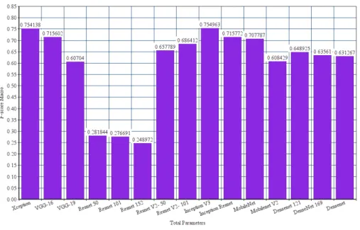
The 𝐹1-score is closer to Precision than Recall with the ResNet being the worst performing model at 0.281844, 0.276691 and 0.248972 (see Figure 9 and Figure 10 ). InceptionV3 and Xception have performed the best overall with 0.754963 and
A Kumar
FIGURE 9 Comparison between pretrained D.L. multi-label classifiers on 𝐹1-score (Macro)
FIGURE 10 Comparison between pretrained D.L. multi-label classifiers on 𝐹1-score (samples)
0.754138 𝐹1 respectively. ResNet50V2 has a higher 𝐹1-score than ResNet50 by 67.15% and ResNet101V2 has a higher 𝐹1 -score than ResNet101 by 59.7%. InceptionV3 outperforms InceptionResnetV2 by 5.19%. Hence a multi-modal architecture outweights the shortcut strategy of ResNets in this case. ResNetV2 has slightly a better 𝐹1-score than DenseNet on an average by 1.11%. Hence layer depth is not too high to account for much decay. Xception architecture also performs better than every
other architecture except InceptionV3. It outperforms MobileNet and MobileNetV2 by 6.14% and 19.32% respectively. This can be because of the lightweight architecture of the MobileNet. ResNet continues to be the worst performing network for 𝐹1-score Samples. VGG-16 and VGG-19 have improved values by 9.12% and 15.57% respectively.
5.3
Analysis of threshold
The optimum solutions were achieved for each model in the threshold values mentioned in the figure. The highest threshold is for VGG19 at 0.18, and the least is for ResNet101 and ResNet152 for 0.001. VGG16 has a threshold of 44.44% lesser at 0.1, the same as that of the Xception and ResNet101V2 network. ResNet50 has the second least threshold at 0.01, 10 times more than ResNet101 and ResNet152. ResNet50V2 has the second-highest threshold at 0.15. InceptionV3 has a threshold at half of the ResNet101V2 at 0.05, while InceptionResNetV2’s threshold lies somewhere between the two at 0.08. MobileNet’s 0.1 threshold is the same as Xception and higher than MobileNetV2. DenseNet121 and DenseNet169 have values of 0.04 and 0.1 respectively (see Figure 11 ).
FIGURE 11 Comparison between pretrained D.L. multi-label classifiers on Threshold
5.4
Analysis of total parameters
The number of elements in the network is called the parameters. These parameters may or may not be adjusted during back-propagation. As the network becomes denser, the number of parameters increases. As is clear from the graph, ResNet has more parameters than ResNetV2 by 22912 parameters for 50 layers. Similarly, for 101 layers, the number of parameters exceeds by 31616. InceptionResnetV2 has 32525248 more parameters than InceptionV3. Xception has 17650024 more parameters than its counterpart MobileNet. Similarly, DenseNet121, even with more layers, has lesser parameters than ResNet101 by 35638080.
5.5
Analysis of non-trainable parameters
Non-trainable parameters are those whose weights are frozen and do not change in back-propagation. These can also be the result of batch normalization, where layers are frozen. ResNet152 has the highest number of non-trainable parameters, 6.91% more
A Kumar
than InceptionResnetV2 coming in second place. MobileNet, with its light features, has 84.52% lesser non-trainable parameters than Xception. DenseNet121 has 87.94% lesser non-trainable parameters than ResNet152.
5.6
Analysis of trainable parameters
Xception and all ResNet networks except InceptionResNetV2 have 34833 trainable parameters. InceptionResNetV2 has 24.98% lesser trainable parameters. VGG has the least with only 8721 such parameters. MobileNet has 49.97% lesser trainable parameters. DenseNet and DenseNet121 have 6.19% and 49.97% lesser parameters than the top 7 networks.
5.7
Summary of Results
Table 4 summarizes the results of the paper. Inception based architectures had optimal results in comparison with other models. The baseline model42obtains precision: 0.76, Precision samples: 0.75, Recall: 0.69, Recall samples: 0.69,
Macro-𝐹1: 0.69, 𝐹1 samples: 0.72. In the literature, it is the only paper that analyses the U.C.M.E.R.C.E.D. dataset for multi-label classification. However, the graph convolutional network it uses requires 2,50,000 epochs for training. Comparatively, the models used in the current paper achieve similar accuracy utilizing ten epochs.
TABLE 4 Quantitative and qualitative results of models
Model Macro-Precision Precision
samples Macro-Recall Recall samples Macro-𝐹1 𝐹1 samples Total
parameters Non-trainable Trainable Threshold
Xception 0.88 0.81 0.7 0.76 0.75 0.76 20896313 20861480 34833 0.1 VGG16 0.76 0.77 0.74 0.85 0.72 0.79 14723409 14714688 8721 0.1 VGG19 0.8 0.86 0.55 0.65 0.61 0.72 20033105 20024384 8721 0.18 ResNet50 0.19 0.19 0.98 0.98 0.28 0.31 23622545 23587712 34833 0.001 ResNet101 0.19 0.2 0.9 0.96 0.27 0.32 42693009 42658176 34833 0.001 ResNet152 0.18 0.23 0.73 0.88 0.25 0.35 58405777 58370944 34833 0.001 ResNet50V2 0.92 0.85 0.58 0.63 0.66 0.7 23599633 23564800 34833 0.15 ResNet101V2 0.9 0.84 0.62 0.69 0.69 0.73 42661393 42626560 34833 0.1 InceptionV3 0.85 0.77 0.75 0.84 0.75 0.77 21837617 21802784 34833 0.05 InceptionResNet 0.87 0.82 0.69 0.73 0.72 0.74 54362865 54336736 26129 0.08 MobileNet 0.81 0.84 0.69 0.77 0.71 0.78 3246289 3228864 17425 0.1 MobileNetV2 0.72 0.65 0.67 0.81 0.61 0.68 2279761 2257984 21777 0.05 DenseNet121 0.59 0.53 0.85 0.95 0.64 0.65 7054929 7037504 17425 0.04 DenseNet169 0.81 0.73 0.63 0.74 0.63 0.71 12671185 12642880 28305 0.1 DenseNet201 0.75 0.63 0.72 0.87 0.63 0.70 18354641 18321984 32657 0.05
6
CONCLUSION AND FUTURE WORKS
In distinction to the predominant single label terrain identification techniques, the current inquiry argues the usefulness of multi-label classifications for V.H.R. R.S. terrestrial visuals for the resolution of terrain classification. This challenging task is comparatively unexplored in literature. Hence, to overcome this research gap, 16 D.L. architectures were pre-trained on ImageNet and further fine-tuned using additional layers for the task of multi-label scene classification. The intuition behind this approach was that pre-trained models would minimize the need for large amounts of V.H.R. image data. Additionally, fine-tuning would improve performance on the multi-label classification taskâĂŤempirical analysis derived on the multi-label U.C.L.U. Image dataset was favorable to pursue this line of investigation.
Fine-tuning the pre-trained deep learning models on the V.H.R. dataset performed well for some specific models. To elaborate on the results, considering 𝐹1-score as a viable metric, InceptionV3 gave the best performance at 0.7549 with a Precision Macro of 0.850155 and a Recall Macro of 0.79955. Xception architecture gave a good result of 0.754138 with a Macro Precision of 0.838788 and a Macro Recall of 0.701278. The ResNet architecture was the worst performing with Macro 𝐹1-scores of 0.281844, 0.276691, and 0.248972 for layers 50, 101, and 152, respectively. MobileNet and MobileNetV2 achieved a Macro 𝐹1 -score of 0.707787 and 0.608429, respectively, which can be attributed to their lightweight architecture having the least number
of parameters at 3246289 and 2279761 only. DenseNet did not perform any better than ResNet with average DenseNet Macro
𝐹1-score at 63.86% and that of ResNetV2 being 67.21%.
The 𝐹1-score achieved can be further improved through optimization techniques. There are cases when V.H.R. images might not be available like in satellite images, and hence accuracy might drop. A separate model for a dataset of Low-Resolution images can be developed. Further, the reason for the high variance in the metrics can be investigated. Network architectures like ResNet giving a Macro 𝐹1-score as low as 0.276691 is a cause of concern when its counterpart ResNet101V2 has a Macro
𝐹1-score of 0.686412. Apart from that, a ratio of non-trainable parameters to the total parameters can be compared among each network architecture and investigated.
References
1. Saadi M, Saeed Z, Ahmad T, Saleem MK, Wuttisittikulkij L. Visible light-based indoor localization using k-means clustering and linear regression. Transactions on Emerging Telecommunications Technologies 2019; 30(2): e3480. 2. Butt TA. Context-aware cognitive disaster management using fog-based Internet of Things. Transactions on Emerging
Telecommunications Technologies2019: e3646.
3. Elbes M, Alrawashdeh T, Almaita E, AlZu’bi S, Jararweh Y. A platform for power management based on indoor localization in smart buildings using long short-term neural networks. Transactions on Emerging Telecommunications Technologies 2020: e3867.
4. Scott G, England M, Starms W, Marcum R, Davis C. Training deep convolutional neural networks for land–cover classification of high-resolution imagery. IEEE Geoscience and Remote Sensing Letters 2017; 14(4): 549–553.
5. Ma S, Lee H. Improving positioning accuracy based on self-organizing map (SOM) and inter-vehicular communication.
Transactions on Emerging Telecommunications Technologies2019; 30(9): e3733.
6. Weng Q, Mao Z, Lin J, Guo W. Land-use classification via extreme learning classifier based on deep convolutional features.
IEEE Geoscience and Remote Sensing Letters2017; 14(5): 704–708.
7. Yang Y, Newsam S. Bag-of-visual-words and spatial extensions for land-use classification. In: ACM. ; 2010: 270–279. 8. Barcelo-Arroyo F, Martin-Escalona I, Manente C. A field study on the fusion of terrestrial and satellite location methods
in urban cellular networks. European transactions on telecommunications 2010; 21(7): 632–639.
9. Liu X. Analysis in big data of satellite communication network based on machine learning algorithms. Transactions on
Emerging Telecommunications Technologies2020: e3861.
10. Rajmohan G, Chinnappan CV, William ADJ, Balakrishnan SC, Muthu BA, Manogaran G. Revamping land coverage analysis using aerial satellite image mapping. Transactions on Emerging Telecommunications Technologies 2020.
11. Zhang F, Du B, Zhang L. Saliency-guided unsupervised feature learning for scene classification. IEEE transactions on
Geoscience and Remote Sensing2014; 53(4): 2175–2184.
12. Zhang F, Du B, Zhang L. Scene classification via a gradient boosting random convolutional network framework. IEEE
Transactions on Geoscience and Remote Sensing2015; 54(3): 1793–1802.
13. Marmanis D, Datcu M, Esch T, Stilla U. Deep learning earth observation classification using ImageNet pretrained networks.
IEEE Geoscience and Remote Sensing Letters2015; 13(1): 105–109.
14. Wu H, Liu B, Su W, Zhang W, Sun J. Deep filter banks for land-use scene classification. IEEE Geoscience and Remote
Sensing Letters2016; 13(12): 1895–1899.
15. Zhang L, Zhang L, Du B. Deep learning for remote sensing data: A technical tutorial on the state of the art. IEEE Geoscience
A Kumar
16. Nerurkar P, Shirke A, Chandane M, Bhirud S. A novel heuristic for evolutionary clustering. Procedia Computer Science 2018; 125: 780–789.
17. Nerurkar P, Shirke A, Chandane M, Bhirud S. Empirical analysis of data clustering algorithms. Procedia Computer Science 2018; 125: 770–779.
18. Aptoula E. Remote sensing image retrieval with global morphological texture descriptors. IEEE transactions on geoscience
and remote sensing2013; 52(5): 3023–3034.
19. Gueguen L. Classifying compound structures in satellite images: A compressed representation for fast queries. IEEE
Transactions on Geoscience and Remote Sensing2014; 53(4): 1803–1818.
20. He N, Fang L, Li S, Plara A. Covariance Matrix Based Feature Fusion for Scene Classification. In: IEEE. ; 2018: 3587–3590. 21. Kumar S, Jain S, Zaveri T. Parallel approach to expedite morphological feature extraction of remote sensing images for cbir
system. In: IEEE. ; 2014: 2471–2474.
22. Fan J, Chen T, Lu S. Unsupervised feature learning for land-use scene recognition. IEEE Transactions on Geoscience and
Remote Sensing2017; 55(4): 2250–2261.
23. Luus F, Salmon B, Bergh V. dF, Maharaj B, Tikanath J. Multiview deep learning for land-use classification. IEEE
Geoscience and Remote Sensing Letters2015; 12(12): 2448–2452.
24. Stivaktakis R, Tsagkatakis G, Tsakalides P. Deep Learning for Multilabel Land Cover Scene Categorization Using Data Augmentation. IEEE Geoscience and Remote Sensing Letters 2019.
25. Bergado J, Persello C, Stein A. Recurrent multiresolution convolutional networks for VHR image classification. IEEE
transactions on geoscience and remote sensing2018(99): 1–14.
26. Gong Z, Zhong P, Hu W, Hua Y. Joint Learning of the Center Points and Deep Metrics for Land-Use Classification in Remote Sensing. Remote Sensing 2019; 11(1): 76.
27. Cao C, Dragićević S, Li S. Land-Use Change Detection with Convolutional Neural Network Methods. Environments 2019; 6(2): 25.
28. Minetto R, Segundo M, Sarkar S. Hydra: an ensemble of convolutional neural networks for geospatial land classification.
IEEE Transactions on Geoscience and Remote Sensing2019.
29. Parmar H. Land Use Classification Using Multi-neighborhood LBPs. arXiv preprint arXiv:1902.03240 2019.
30. Karalas K, Tsagkatakis G, Zervakis M, Tsakalides P. Land classification using remotely sensed data: Going multilabel.
IEEE Transactions on Geoscience and Remote Sensing2016; 54(6): 3548–3563.
31. Zhen Y, Liu H, Li J, Hu C, Pan J. Remote sensing image object recognition based on convolutional neural network. In: IEEE. ; 2017: 1–4.
32. Flores E, Zortea M, Scharcanski J. Dictionaries of deep features for land-use scene classification of very high spatial resolution images. Pattern Recognition 2019; 89: 32–44.
33. Uba N. Land use and land cover classification using deep learning techniques. arXiv preprint arXiv:1905.00510 2019. 34. Castelluccio M, Poggi G, Sansone C, Verdoliva L. Land use classification in remote sensing images by convolutional neural
networks. arXiv preprint arXiv:1508.00092 2015.
35. Li J, Lin D, Wang Y, Xu G, Ding C. Deep Discriminative Representation Learning with Attention Map for Scene Classification. arXiv preprint arXiv:1902.07967 2019.
36. Simonyan K, Zisserman A. Very deep convolutional networks for large-scale image recognition. arXiv preprint
37. He K, Zhang X, Ren S, Sun J. Deep residual learning for image recognition. arXiv preprint arXiv:1512.03385 2015. 38. Szegedy C, Liu W, Jia Y, et al. Going deeper with convolutions. In: ; 2015: 1–9.
39. Chollet F, others . Keras. https://keras.io; 2015.
40. Howard A, Zhu M, Chen B, et al. Mobilenets: Efficient convolutional neural networks for mobile vision applications. arXiv
preprint arXiv:1704.048612017.
41. Huang G, Liu Z, Van Der Maaten L, Weinberger K. Densely connected convolutional networks. In: ; 2017: 4700–4708. 42. Khan N, Chaudhuri U, Banerjee B, Chaudhuri S. Graph convolutional network for multi-label VHR remote sensing scene
recognition. Neurocomputing 2019; 357: 36–46.
How to cite this article: A. Kumar, K. Abhishek, A. Singh, P. Nerurkar, M. Chandane, S. Bhirud, D. Patel, and Y. Busnel