Improving NILM by Combining Sensor Data and Linear Programming

HAL Id: hal-02394920

https://hal.inria.fr/hal-02394920

Submitted on 5 Dec 2019

HAL is a multi-disciplinary open access

archive for the deposit and dissemination of

sci-entific research documents, whether they are

pub-lished or not. The documents may come from

teaching and research institutions in France or

abroad, or from public or private research centers.

L’archive ouverte pluridisciplinaire HAL, est

destinée au dépôt et à la diffusion de documents

scientifiques de niveau recherche, publiés ou non,

émanant des établissements d’enseignement et de

recherche français ou étrangers, des laboratoires

publics ou privés.

Improving NILM by Combining Sensor Data and Linear

Programming

Nicolas Roux, Baptiste Vrigneau, Olivier Sentieys

To cite this version:

Nicolas Roux, Baptiste Vrigneau, Olivier Sentieys. Improving NILM by Combining Sensor Data and

Linear Programming. SAS 2019 - IEEE Sensors Applications Symposium, Mar 2019, Sophia Antipolis,

France. pp.1-6, �10.1109/SAS.2019.8706021�. �hal-02394920�

Improving NILM by Combining Sensor Data and

Linear Programming

Nicolas Roux

, Baptiste Vrigneau

, and Olivier Sentieys

†_{Univ Rennes, CNRS, IRISA, Lannion, France} Email: {firstname.lastname}@irisa.fr

Abstract—Knowing the plug-level power consumption of each appliance in a building can lead to drastic savings in en-ergy consumption. Non-Intrusive Load Monitoring (NILM) is a method for disaggregating power loads in a building to the single appliance level, without using direct sensors or electric meters attached to each device. This paper addresses the issues of NILM inaccuracy in the context of industrial or commercial buildings, by combining data from a low-cost, general-purpose, wireless sensor network. A novel approach to tackle this issue is proposed, using a simplex-based solver, to estimate the power load values of the steady states on sliding windows of data with varying size. In this paper, we show the principle of the approach and demonstrate its interest, limited complexity, and ease of use. Index Terms—Smart Buildings, Non-Intrusive Load Monitor-ing, Wireless Sensor Network

I. INTRODUCTION

Developing smarter/greener electric grids has been an ex-panding field of research over the last decades. One of the essential requirements for energy utilities is the knowledge of power consumption patterns at the single-appliance level. To estimate these patterns without using an individual power me-ter for each appliance, Non-Intrusive Load Monitoring (NILM) consists in disaggregating electrical loads by examining the appliance specific power consumption signature within the aggregated load single measurement. Therefore, the method is considered non-intrusive since the data is collected from a single electrical panel outside of the monitored building. Thus, NILM has been a very active field of research with renewed interest over the last years [16].

A lot of research has been made on residential power disaggregation, due to the growth of home smart meters, and likely uniqueness of most relevant appliances. Nevertheless, NILM techniques applied to industrial or commercial build-ings still face many challenges. One eloquent example is the multiplicity of users and appliances or specific devices. Some companies already offer solutions to evaluate and reduce consumption of buildings and, recently, for personal residence. However, a key-point of NILM algorithms is the power estimation of each device states. Of course, a dispersion exists for a given type of load and it is obvious that a fridge will be different on each home. Moreover, it permits one to detect an abnormal behaviour and alert on a possible breakdown. In this work, we propose a novel approach to solve this problem based on a linear algebra formulation. We formulate

the disaggregation problem as a convex, linear programming problem, with complete or partial knowledge of additional variables, naming the device states matrix. Information to solve the problem comes not only from the total power consumption, but also from low-cost wireless sensors. Indeed, the algorithm will be validated using open datasets, as well as using our Smart Building platform, called SmartSense, which collects data from individual and global power meter and from various sensors.

The paper is organized as follows. In Section II, we briefly introduce the state of the art. Section III formulates the problem, before introducing the numerical solving methods in Section IV. Finally, we describe and analyze results in Section V, as well as some methods to reduce complexity.

II. RELATEDWORK

More than two decades ago, G.W. Hart initiated research on NILM [6]. He introduced the concept of estimating individual appliance power consumption without relying on individual direct metering. Since, researchers strived to find ways to improve NILM accuracy and solve its limitations. Basically, NILM is a source separation problem where a set of appliances consume an aggregated amount of power. The end goal is to evaluate the power consumption and the state of each appliance based on the sole reading of the aggregated power consumption. For this reason the term ”disaggregated” is often used to describe a solved NILM problem [18]. The original NILM concept is described in Figure 1. As an example, a fan heater is switched on at t = 10min until t = 28min and then a blender is switched on at t = 17min. The first problem is to detect the instant where these appliances are switched on and off based on their electrical signature: activation height, length, or shapes that are pictured with arrows. A second problem is to estimate their power loads from this trace. This is the main problem addressed in this paper. Finally, this estimation could also be used to detect if an appliance is in fault or aging (unusual activation shape).

Various approaches have been considered with interesting results. In [17], the author uses a probabilistic approach to tackle this challenge. Recently, machine learning methods, especially deep neural networks, have shown significant im-provements in classification problems over the last few years and was applied to improve NILM in [5], [7].

This full text paper was peer-reviewed at the direction of IEEE Instrumentation and Measurement Society prior to the acceptance and publication.

Fig. 1: Non-Intrusive Appliance Load Monitoring as introduced in [6].

Furthermore, interest of energy disaggregation has been dis-cussed in [2] with remarkable potential annual energy savings due to an individual appliance feedback (more than 12%) Meanwhile, extensive works at the University of California San Diego have been made to determine the role of Smart Buildings on energy savings on an university campus [1] [15]. This confirms both environmental and economical purposes of NILM and smart buildings automation in general.

Environmental sensing and additional heterogeneous infor-mation can be exploited to address some of the prevailing chal-lenges faced by the current NILM techniques [19]. However, this comes at the cost of an increased complexity. Therefore, load monitoring combining extra information with the power consumption of the whole building, seems like the right way to go. Moreover, with the increasing number of smart sensors in buildings deployed for multiple purposes, collecting this kind of data without additional installation has become more and more plausible. This can explain the recent interest in this kind of approach. For example, in [4], the authors suggested incorporating time-of-day usage patterns into disaggregation algorithms to improve accuracy and reduce computational complexity.

All over the globe, many efforts have been made to im-prove energy efficiency of university campus infrastructures through the use of Internet of Things (IoT) solutions [14]. More and more universities (e.g., Lisbon Instituto Superior T´ecnico, Helsinki University of Applied Sciences, Politecnico di Milano, Lule˚a Technical University) launched pilot projects to measure the impact of IoT solutions on their energy consumption. For example, the Lisbon Pilot proposed a digital vote system via student’s smartphones to set the auditorium lighting and HVAC settings to a satisfying level.

In [11], the author propose several methods to improve NILM algorithm performance with the use of data extracted from sensors networks. Using these environmental sensors, and testing several algorithms, the authors concluded that monitoring a few appliances could drastically improve NILM performance. Detecting the state of an appliance with the adequate sensors can be a low-complexity task. For example,

the operation of a workplace printer may be readily recognized with an audio sensor. Lights can be easily monitored by sensors as well. Assuming the state of an appliance is known, an interesting task is then to estimate the characteristics of steady-state power of an appliance, on a length-significant power trace. In their work around ViridiScope [9], the authors implemented a power monitoring system by indirect sensing with self-learning automatic calibration of each sensor.

In this paper, our objective is to set the ground for a multi-purpose, low-cost sensor network to improve the accuracy of NILM algorithms. As opposed to some Semi-Intrusive Load Monitoring techniques like Viridiscope, we aim to use general information about the target environment (temperature, room occupancy, and such) rather than dedicated sensing.

III. DISAGGREGATINGAPPLIANCEPOWERLOADS A. Problem Statement

A basic problem of NILM is disaggregating the main power load of a building. We consider a low-rate sampling (typically 1Hz) and our approach is based on formulating the disaggregation as an optimization problem, which consists in minimizing the difference between the main power meter output and the sum of disaggregated reconstructed appliances. We use the term disaggregated for an appliance whose steady-state temporal steady-state matrix si,j(t) is known, and steady-state

power values in Watts (W) wi,j need to be estimated. The

problem can then be written as min wi,j kxtot(t) − N X i=1 Mi X j=1 wi,j× si,j(t)kd (1) with

• xtot the main power of the building, • N the number of appliances,

• Mi the number of steady states per appliance i,

• wi,j power consumption of appliance i in steady-state j, • si,j(t) ∈ {0, 1} a boolean equal to 1 when appliance i is

in state j, and

• k.kd a given norm. In this work, we consider l1-norm or

absolute value.

Note that the optimization-based NILM approach often tries to solve the mirror problem of (1)

min si,j(t) kxtot(t) − N X i=1 Mi X j=1 wi,j× si,j(t)kd (2)

to estimate the states of the devices, knowing each individual power load. To sum up, knowing partial information on the states of the appliance, we aim to estimate the power values of appliance wi,j.

B. Environment Description

To estimate the state matrix of an appliance, we use Smart-Sense, a fine grained, multi-modal sensor network platform. SmartSense is a research platform based on a sensor network designed for various data acquisition. Each network node

Fig. 2: A map of the physical network mesh, each blue shape being a standard SmartSense node, each red shape being a SmartSense node including an IR sensor, and each yellow square an electrical sub-meter attached to an electrical panel.

is composed of fifteen sensors to retrieve a wide range of information, including:

• Video sensors (Video-Graphic-Array (VGA) and Infra-Red (IR) cameras) and audio sensors.

• Radio sensors (2.4 GHz, Sub-GHz, and Ultra-Wide-Band) to sense the radio-frequency band occupancy and to estimate positions.

• Air quality sensors (temperature, humidity, carbon dioxide concentration, air pressure, etc.).

• Light sensors (Ultraviolet and Red-Green-Blue-White). • Distance sensor (Laser telemeter).

SmartSense is composed of more than 150 nodes disseminated in rooms ranging from 9 to 40 square meters and corridors. The mesh of the sensor network is quite dense, with from two to four nodes in each room, according to the room surface. The frequency of the data acquisition will vary according to the data nature. For example, air quality sensor data do not need to be retrieved as frequently as audio or light sensor data. The SmartSense physical network is currently deployed in our laboratory. An example of a deployment map in a sub-network of SmartSense is depicted in Figure 2.

Having an overly dense network is purposeful for a research-oriented sensor network. Indeed, oversizing the net-work will allow us to artificially undersample the data, there-fore deducing how much downsizing can be applied while keeping disagreggation quality acceptable. While the exper-imental setup will provide around two to four sensors per room, a realistic expectation for an industrial NILM solution in commercial buildings would probably contain about one sensor node for small rooms (office) and two or more nodes for bigger rooms (e.g., cafeteria, meeting rooms, corridors).

Moreover, since the whole raw data cannot realistically be retrieved from the sensor nodes to the main system, some pre-processing is performed by the network node itself. Therefore, the pre-processing has to be chosen carefully, according to the data final use. Not all of the above sensors are relevant for NILM. The purpose of the SmartSense platform is also to provide scientists with a wide diversity of data for research around the topic of Smart Buildings and data mining. Since SmartSense data is not yet available (the platform should

be deployed in Spring 2019), our algorithms have first been tested on the Reference Energy Disaggregation Data Set (REDD) [10] and we hope to extend to other datasets such as the UK-DALE dataset [8] and the AMPds [13].

To sum up, a first estimation of the state matrix is obtained via an environmental sensors network which, after retrieving the data gives us a first rough estimate of the monitored appliances states.

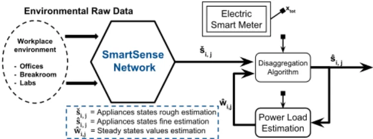
IV. SOLVING THEDISAGGREGATIONPROBLEM In the case of NILM, SmartSense raw data will be used such as described schematically in Figure 3. The total power of the building xtotis read from a smart power meter sampled

at 1 Hz.

The raw environmental data (audio, luminosity, etc.) Dk,lis

acquired by SmartSense nodes. For network load and privacy issues, these raw data are not retrieved from the sensor by the main system. Instead, each node processes individually a rough estimation of the state ˇs of the monitored appliances. Given ˇs and xtot, a classical NILM disaggregation algorithm

is run to determine a better estimation of the partial steady states ˆs. Given ˆs and xtot, the individual power load estimation

of steady states determines w for each monitored appliance,_b which improves the accuracy of the next iterations of the previous step. More iteration steps can be performed for each sample of xtotto increase accuracy at the cost of computation

complexity.

As mentioned in Section III, our problem is based on study-ing the steady states of various appliances. To evaluate the accuracy of our algorithm, we use the experimental protocol depicted in Figure 4 and detailed below.

First, the raw data are extracted from REDD. The chan-nel i.dat files contain time-stamped power metering infor-mation for single appliances or small circuit of same type appliances, for example a small lighting circuit or kitchen outlets. To define a reference for appliance steady states, we then process each appliance individually with a python script. To perform this, we use a custom 1-D edge detection algorithm for detecting steady states locations. Then, the whole individual power trace is clustered into a list of known steady states, to simulate the a priori knowledge of appliances states. Results of this experiment are collected and used as a reference for our further experiments. This is due to the fact that results are obtained from the individual power traces of REDD

Workplace environment - Offices - Breakroom - Labs Disaggregation Algorithm Power Load Estimation Electric Smart Meter

Environmental Raw Data

š_{i, j} xtot ŝi, j ŵ_i,j ši, j = Appliances states rough estimation ŝi, j = Appliances states fine estimation ŵi,j = Steady states values estimation

SmartSense Network

Fig. 3: Representation of the role of power load estimation in the full scope of the SmartSense usage for NILM.

appliances, and thus are more accurate than disaggregated power characteristics.

To detail our approach, we first clear the data from noise with a median filter, to obtain clear distinguishable edges, as in Figure 1 but for one appliance only. Then, edge detection is applied to distinguish the appliance states changes. When an edge is found and the appliance maintains a steady state for a certain time (determined by the nature of the appliance), we consider having observed a ”steady state”. We then compare the new power level with the known steady power levels of the appliance. If no match can be found within a certain margin (arbitrary at first, but dynamic then), a new power level is added to the known power levels of this appliance. We also count the number of samples which correspond to each steady power level, which allows us to compress the power data : after the power trace has been processed, it can be mapped into a steady states matrix, and a power signature vector. The goal of our next step is to retrieve the power signature vector of a single appliance from the aggregated power of a whole system (like the REDD houses from our test dataset), and the state matrix of the target appliance.

Knowing the state matrix of studied appliances and main power through individual classification (see Figure 4), we use the GNU Linear Programming Kit (GLPK) [12] to execute an optimization script. GLPK offers a variety of programming tools including the GNU MathProg high-level language able to design and solve mathematical problems on the fly. Although not being used yet in the NILM literature, its ease of use, along its ability to write on the fly optimization scripts with log files for efficient debugging makes it a relevant choice for NILM problems. To solve the optimization problem, we use the simplex algorithm, which performs best when upper and lower bounds on the optimization solution are known.

In our case, the optimization script is generated

automat-REDD Dataset House k k ∈ [1:6] channel_i.dat i ∈ [1 : 20] wreference( i, j) ŵi,j xtot states_matrix Classification script Pre-processing script GLPK script labels.dat

Fig. 4: The three steps of our experimental protocol to estimate power loads from main power trace and validating the results with individual power loads references.

ically by the classification process : after the data batch has been processed, the states matrix is eventually altered (to inject error) and exported to be GLPK-readable (to simulate the data from SmartSense sensors). The optimization is then handled by the GLPK solver and its result is processed to be readable by our classification script, therefore allowing data windowing, as seen in the next section.

V. REDUCINGOPTIMIZATIONCOMPLEXITY Since linear optimization can be a computing-intensive task and it is desirable to run the actions described in Figure 4 in real time, the complexity of the problem must be reduced as much as possible without affecting the accuracy of the power estimation or the disaggregation. Two methods are introduced to reduce complexity: windowing the power trace, and pre-processing the data according to the state matrix to remove redundant information.

A. Windowing

To reduce the size of the optimization problem, and there-fore to allow for the application to run in real-time, data are processed inside a time window. The first issue to address when using windowed data instead of the whole available dataset is how to take account of information from the previous windows when processing the optimization problem of the next window. To achieve this, in the GLPK optimization file, we set lower and upper boundaries based on the previous optimized results, and an arbitrary tolerance, which is typically set around ±10%.

The next important step is how to choose the size of the window. Through our experiments, we noticed that the first window should be significantly longer, e.g. one day, while the next windows could be significantly lower, e.g. half an hour, without losing accuracy. This also allows for a dynamic tracking of characteristic power loads, which can be interesting for detecting quickly and pinpointing temporally a faulty appliance. Different singular window lengths and their corresponding execution times are detailed in Figure 5. While

25000 50000 75000 100000 125000 150000 175000 Window length (s) 0 200 400 600 800 Execution time (s)

Fig. 5: Optimization script execution time as a function of the window length, running on an Intel(R) Core(TM) i7-6600U CPU @ 2.60GHz with three seconds between each sample.

shorter windows are useful for a dynamic monitoring of our appliances, a too short window can make it harder to observe all the states of an appliance and obtain the characteristic steady states values. Figure 6 collects the number of observed states, relatively to the window length.

0 2000 4000 6000 8000 Window length (s) 1.5 2.0 2.5 3.0 3.5 4.0 Mean observ ed states coun t

Fig. 6: Evolution of the number of states observed relatively to the window observation length for 100 random individual windows (no communication from window to window) for various bathroom appliances. All appliances have a total of four different states. This hints that even a long window length cannot guarantee a complete observation of all the states of the appliances.

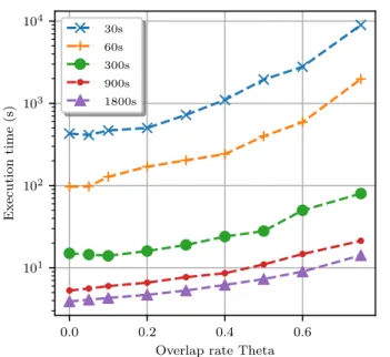
Finally, we define the reactivity r as follows : r = T (1 − θ)

with T the window length (in seconds) and θ the overlap rate of subsequential windows. Reactivity and window subsequen-tiality are pictured in Figure 7. Full classification execution times are displayed in Figure 8. As expected, execution time grows exponentially with the overlap rate. It is also worth

Window 1 Window 2 Time (s) Power (W) θ * T r Device signature

Fig. 7: Visualization of the reactivity r and the overlap rate θ. The devices signature are extracted from each window and transmitted as a reference for a better disaggregation of the next window.

mentioning that while having no significant impact on disag-gregation performance, the overlapping rate θ is proportional to the reactivity r. In a real-case scenario (building energy management), being able to acknowledge in real time the individual activity of each appliance as accurately as possible

0.0 0.2 0.4 0.6

Overlap rate Theta 101 102 103 104 Execution time (s) 30s 60s 300s 900s 1800s

Fig. 8: Overlap parameter θ (x-axis) and window length (plots) influence on execution time (Log-scale) to disaggregated a whole day of windowed data.

could be particularly useful (i.e. fault-detection for sensitive appliance) or marginally interesting if the NILM purpose is to monitor only daily energy trends.

B. Data Pre-Processing

Even when using small windows of data, computation can be sped-up by pre-processing the data. To perform this task, we scan the data window looking for duplicate samples, i.e. time samples with the very same state row, and a xtotsimilar

power value with a very low tolerance, e.g., 1W.

If a duplicate of a row is found, we remove the duplicate and increment a duplicate counter of the state/power value combination. This is a sort of compression of the states matrix, with a loose tolerance (1 W). Pre-processing is done after the computation of the states matrix (see Figure 4), and tends to reduce the size of this matrix with the intent to reduce both linear optimization computation time and the storage requirement of NILM. This pre-processing is the most time consuming task of our program, but the execution time is drastically decreased by this technique which is no more than a trivial duplicate search.

Overall, we noticed that while windowing is needed to ensure the adaptability of our system to real-time data, the pre-processing task is the most efficient way of reducing execution time.

C. Comparison with Related Work

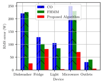
In this section, we compare our algorithm performance with state of the arts algorithms provided by the NILM-ToolKit [3] benchmark tool. Figure 9 compares the performance of our approach with two state-of-the-art algorithms. We use the Root-Mean-Square (RMS) Error between the predicted and

true power trace as our reference metric, which is used by the NILM community to compare algorithms [3]. The target appliances are the five most consuming devices of the REDD1 dataset. On average, we can see a 71.28% decrease in RMS error over these five appliances, compared with the best state-of-the-art algorithm for each appliance. However, we can see that the decrease is not homogeneous, with a maximum improvement for the house light circuit (over 96% RMS decrease), but only 19% decrease for the fridge appliance. This is caused by the shape of the appliance power traces : a steadier appliance like a lighting system is much more favorable to our approach because of our edge detection-based algorithm.

It is worth mentionning that despite the clear improvement in performance over the RMS error, the algorithms we com-pare to do not use additional data as we did (appliance state knowledge through pre-processing). Nevertheless, the perfor-mance improvement is promising and confirms the interest in adding sensor data to NILM.

Dishwasher Fridge Light Microwave Outlets Device 0 50 100 150 200 250 RMS error (W) CO FHMM Proposed Algorithm

Fig. 9: Prediction results on REDD data with simulated sensors information, compared to Combinatorial Optimization and Factorial Hidden Markov Model algorithms

VI. CONCLUSION

In this paper, we present some work around Non-Intrusive Load Monitoring using a hybrid reverse approach via the SmartSense platform. Environmental information is used to infer the steady states of monitored appliances, and an optimization-based method is used to estimate the charac-teristic power loads of the steady states. While our method has been used on labeled datasets at the moment, future work will include the uncertainty around steady states, and processing of environmental SmartSense data. Further results and the complete dataset will be released in the near future on SmartSense website.

ACKNOWLEDGMENT

This work is supported by the European Union through the European Regional Development Fund (ERDF), and by Ministry

of Higher Education and Research, Brittany and Rennes Metropole, through the CPER Project SOPHIE - STIC & Ondes.

REFERENCES

[1] Yuvraj Agarwal, Bharathan Balaji, Rajesh Gupta, Jacob Lyles, Michael Wei, and Thomas Weng. Occupancy-driven energy management for smart building automation. In Proceedings of the 2nd ACM Workshop on Embedded Sensing Systems for Energy-Efficiency in Building, pages 1–6, New York, NY, USA, 2010.

[2] K Carrie Armel, Abhay Gupta, Gireesh Shrimali, and Adrian Albert. Is disaggregation the holy grail of energy efficiency? the case of electricity. Energy Policy, 52:213–234, 2013.

[3] Nipun Batra, Jack Kelly, Oliver Parson, Haimonti Dutta, William Knot-tenbelt, Alex Rogers, Amarjeet Singh, and Mani Srivastava. Nilmtk: an open source toolkit for non-intrusive load monitoring. In Proceedings of the 5th international conference on Future energy systems, pages 265–276. ACM, 2014.

[4] Chinthaka Dinesh, Stephen Makonin, and Ivan V Bajic. Incorporating time-of-day usage patterns into non-intrusive load monitoring. In Proc. 5th IEEE Global Conference on Signal and Information Processing (GlobalSIP), 2017.

[5] Pedro Paulo Marques do Nascimento. Application of Deep Learning Techniques on NILM. PhD thesis, Universidade Federal do Rio de Janeiro, 2016.

[6] G.W. Hart. Non-intrusive appliance load monitoring. Proceedings of the IEEE, 80(12):1870–1891, Dec. 1992.

[7] Jack Kelly and William Knottenbelt. Neural nilm: Deep neural networks applied to energy disaggregation. In Proceedings of the 2Nd ACM International Conference on Embedded Systems for Energy-Efficient Built Environments, BuildSys’15, pages 55–64, New York, NY, USA, 2015.

[8] Jack Kelly and William Knottenbelt. The uk-dale dataset, domestic appliance-level electricity demand and whole-house demand from five uk homes. Scientific data, 2:150007, 2015.

[9] Younghun Kim, Thomas Schmid, Zainul M. Charbiwala, and Mani B. Srivastava. Viridiscope: Design and implementation of a fine grained power monitoring system for homes. In Proc. Ubicomp09, pages 245– 254, 2009.

[10] J. Zico Kolter and Matthew J. Johnson. REDD: A public data set for energy disaggregation research. In SustKDD, 2011.

[11] X-C Le. Improving Performance of Non-Intrusive Load Monitoring with Low-Cost Sensor Networks. PhD thesis, University of Rennes, 2017. [12] A Makhoren. Gnu linear programming kit, modeling language GNU

math prog. Department for Applied Informatics, Moscow Aviation Institute, 2005.

[13] Stephen Makonin, Fred Popowich, Lyn Bartram, Bob Gill, and Ivan V Bajic. Ampds: A public dataset for load disaggregation and eco-feedback research. In IEEE Electrical Power & Energy Conference (EPEC), pages 1–6. IEEE, 2013.

[14] Pascal Ravesteyn, Henk Plessius, and Joris Mens. Smart green campus: How it can support sustainability in higher education. In Proceedings of the 10th european conference on management leadership and gover-nance (ECMLG 2014), pages 296–303, 2014.

[15] T. Weng and Y. Agarwal. From buildings to smart buildings-sensing and actuation to improve energy efficiency. Design Test of Computers, IEEE, 29(4):36–44, 2012.

[16] M. Zeifman and K. Roth. Nonintrusive appliance load monitoring: Review and outlook. IEEE Transactions on Consumer Electronics, 57(1):76–84, 2011.

[17] Michael Zeifman. Disaggregation of home energy display data using probabilistic approach. IEEE Transactions on Consumer Electronics, 58(1):23–31, 2012.

[18] Ahmed Zoha, Alexander Gluhak, Muhammad Ali Imran, and Sutharshan Rajasegarar. Non-intrusive load monitoring approaches for disaggregated energy sensing: A survey. Sensors, 12(12):16838–16866, 2012. [19] Ahmed Zoha, Muhammad Ali Imran, Alexander Gluhak, and Michele

Nati. A comparison of generative and discriminative appliance recogni-tion models for load monitoring. In IOP Conference Series: Materials Science and Engineering, volume 51, page 012002. IOP Publishing, 2013.