HAL Id: hal-01887203
https://hal.inria.fr/hal-01887203
Submitted on 3 Oct 2018
HAL is a multi-disciplinary open access
archive for the deposit and dissemination of
sci-entific research documents, whether they are
pub-lished or not. The documents may come from
teaching and research institutions in France or
abroad, or from public or private research centers.
L’archive ouverte pluridisciplinaire HAL, est
destinée au dépôt et à la diffusion de documents
scientifiques de niveau recherche, publiés ou non,
émanant des établissements d’enseignement et de
recherche français ou étrangers, des laboratoires
publics ou privés.
Multicarrier NOMA Systems
Yaru Fu, Lou Salaun, Chi Wan Sung, Chung Shue Chen
To cite this version:
Yaru Fu, Lou Salaun, Chi Wan Sung, Chung Shue Chen. Subcarrier and Power Allocation for the
Downlink of Multicarrier NOMA Systems. IEEE Transactions on Vehicular Technology, Institute of
Electrical and Electronics Engineers, In press, 67 (12), pp.11833-11847. �10.1109/TVT.2018.2875601�.
�hal-01887203�
Subcarrier and Power Allocation for the Downlink
of Multicarrier NOMA Systems
Yaru Fu, Member, IEEE, Lou Sala¨un, Student Member, IEEE,
Chi Wan Sung, Senior Member, IEEE and Chung Shue Chen, Senior Member, IEEE
Abstract—This paper investigates the joint subcarrier and power allocation problem for the downlink of a multi-carrier non-orthogonal multiple access (MC-NOMA) system. A novel three-step resource allocation framework is designed to deal with the sum rate maximization problem. In Step 1, we relax the problem by assuming each of the users can use all subcarriers simultaneously. With this assumption, we prove the convexity of the resultant power control problem and solve it via convex programming tools to get a power vector for each user; In Step 2, we allocate subcarriers to users by a heuristic greedy manner with the obtained power vectors in Step 1; In Step 3, the proposed power control schemes used in Step 1 are applied once more to further improve the system performance with the obtained sub-carrier assignment of Step 2. To solve the maximization problem with fixed subcarrier assignments in both Step 1 and Step 3, a centralized power allocation method based on projected gradient descent algorithm and two distributed power control strategies based respectively on pseudo-gradient algorithm and iterative waterfilling algorithm are investigated. Numerical results show that our proposed three-step resource allocation algorithm could achieve comparable sum rate performance to the existing near-optimal solution with much lower computational complexity and outperforms power controlled OMA scheme. Besides, a tradeoff between user fairness and sum rate performance can be achieved via applying different user power constraint strategies in the proposed algorithm.
Index Terms—Multi-carrier non-orthogonal multiple access (MC-NOMA), successive interference cancellation (SIC), game theory, Nash equilibrium, gradient and pseudo-gradient descent, synchronous iterative waterfilling algorithm (SIWA).
I. INTRODUCTION
In the third generation partnership project Long Term Evolution (3GPP-LTE) and LTE-Advanced (LTE-A) cellu-lar networks, orthogonal frequency division multiple access (OFDMA) has been widely applied, in which the whole system bandwidth is divided into multiple orthogonal subcarriers and each subcarrier is exclusively utilized by at most one user during each time slot at each base station (BS). Therefore, Copyright (c) 2015 IEEE. Personal use of this material is permitted. However, permission to use this material for any other purposes must be obtained from the IEEE by sending a request to pubs-permissions@ieee.org. Y. Fu and C. W. Sung are with the Dept. of Electronic Engineering, City University of Hong Kong, Tat Chee Avenue, Kowloon, Hong Kong SAR (e-mail: yarufu2-c@my.cityu.edu.hk; albert.sung@cityu.edu.hk).
L. Sala¨un and C. S. Chen are with Bell Labs, Nokia
Paris-Saclay, 91620 Nozay, France (e-mail: lou.salaun@nokia-bell-labs.com; chung shue.chen@nokia-bell-labs.com).
This work was partially supported by a grant from the Research Grants Council of the Hong Kong Special Administrative Region, China (Project No. CityU 11216416). A part of the work was carried out at LINCS (www.lincs.fr), and presented at IEEE International Conference on Communications (ICC), May, Paris, 2017 [1].
OFDMA can avoid intra-cell interference by performing user transmission scheduling at the BS. Moreover, it can be imple-mented with low-complexity receivers. However, the spectral efficiency is in general under-utilized due to the requirement of channel access orthogonality.
The mobile data traffic for cellular systems is expected to increase by 1000 folds by 2020, seeking efficient multiple access technologies becomes very important, as it is the key for meeting the dramatically increasing bandwidth demand. Non-orthogonal multiple access (NOMA) has recently received significant attention and has been regarded as a promising candidate for the fifth generation (5G) cellular systems. In contrast to orthogonal multiple access (OMA), NOMA allows the multiplexing of multiple users with different power levels on the same frequency resource block, which provides a higher system spectral efficiency [2], [3].
Since several users are multiplexed on the same subcarrier simultaneously, successive interference cancellation (SIC) is adopted at the receiver side to mitigate the resulting co-channel interference. Therefore, power must be allocated properly among the multiplexed users on each subcarrier such that interfering signals can be correctly decoded and subtracted from the received signal of some users. Fractional transmit power control (FTPC) is a sub-optimal but commonly used power control strategy for users sum rate maximization prob-lems, which allocates power according to the individual link condition of each user [2], [4]. In [5], power allocation in single-cell NOMA system is performed in a fixed manner. In [6] and [7], distributed power allocation algorithms are proposed to minimize total power consumption subject to user data rate constraints for the downlink and uplink multi-cell NOMA systems, respectively. In addition, there exists some other works that investigate the power control for NOMA in heterogeneous networks [8], cooperative systems [9], [10] and multi-antenna scenarios [11], [12]. Except power control, fairness is also an important feature of NOMA. In [13], the resource allocation fairness between NOMA and OMA schemes is compared, based on which a hybrid NOMA-OMA scheme is proposed to further enhance the users fairness. Recent works [14], [15] investigate NOMA with two sets of orthogonal signal waveforms, in which power imbalance between different users’ signals is not needed. Moreover, deep learning has been applied in NOMA to estimate the channel state information by learning the environment automatically via offline learning [16].
For multicarrier NOMA (MC-NOMA) systems, subcarrier assignment and power control for multiplexed users are two
interacted factors for achieving high system performance. The work in [17] demonstrates that in practical LTE cellular systems, MC-NOMA has better system-level downlink per-formance in terms of user throughput than that of OFDMA networks by realistic computer simulation. In [18], a mono-tonic optimization method is proposed to achieve the optimal subcarrier and power allocation for MC-NOMA system. How-ever, it is assumed that each subcarrier can accommodate at most two users, which restricts the application of the designed algorithm. The authors of [19] propose a low-complexity algo-rithm of jointly optimizing subcarrier assignment and power allocation to minimize the total transmit power of OFDM-based NOMA network. In addition, the energy-efficient re-source allocation problems for MC-NOMA systems with perfect channel state information (CSI) and imperfect CSI are investigated in [20] and [21], respectively. An iterative algorithm is provided in [22] to solve the sub-channel and power allocation problem in MC-NOMA network. The de-signed resource allocation strategy is not so efficient as swap-matching is adopted to do the subcarrier assignment during each iteration, especially when the number of user is large. In [23], a greedy user selection and sub-optimal power alloca-tion scheme based on difference-of-convex (DC) programming is presented to maximize the weighted throughput in a two-user NOMA system. It is observable that the scheme has high computational complexity due to the DC programming in optimizing the power allocation among different subcarriers and different users. In [24], various user pairing algorithms for multi-input and single-output (MISO) MC-NOMA system are proposed. However, the performance gain of [24] is limited due to the use of naive power control schemes such as fixed power allocation (FPA) and FTPC among multiplexed users. Besides, a joint power and channel allocation problem for sum rate maximization of MC-NOMA system is formulated in [25], which is shown NP-hard and solved by Lagrangian duality and dynamic programming (LDDP). To gauge the performance of LDDP, the authors investigate the optimality bound on the global optimum and show that LDDP could achieve a close-to-upper-bound performance.
Motivated by the aforementioned observations and the much lower latency requirement of 5G, we propose a time-efficient joint subcarrier and power allocation algorithm for MC-NOMA, which could achieve comparable performance to LDDP. Our main contributions are summarized as follows:
1) A resource allocation framework is designed, which con-sists of the following three steps:
Step 1: Assume each user can use all subcarriers. By this assumption, the problem becomes convex and can be solved efficiently. A centralized or some distributed algorithms for the resultant power control subproblem are designed.
Step 2: Based on the power allocation solution obtained, the subcarrier assignment problem is solved, tak-ing into account practical system constraints. Step 3: Given the above subcarrier allocation, Step 3
solves a convex problem, i.e., the power allo-cation is further adjusted to optimize the final
system performance.
The above 3-step methodology allows us to solve the problem efficiently. This is how we handle the problem, why we do 3 steps. And then, we show its near optimal performance by comprehensive simulation results. 2) In Steps 1 and 3, the subcarrier assignment is fixed. We
prove that the resultant subproblem is convex, which can be optimally solved in a centralized manner via gradient descent algorithm. Alternatively, it can be solved more efficiently in a distributed manner. To do this, we model the problem as a multi-player concave game, and prove the existence and uniqueness of its Nash equilibrium. Two distributed algorithms, namely, pseudo-gradient de-scent and iterative waterfilling, are investigated, and their convergence properties are established. Furthermore, we analyze the asymptotic computational complexity of the proposed power control schemes. Except for the above-mentioned, in Step 2, a heuristic method, which makes use of the result obtained in Step 1, is proposed for subcarrier assignment.
3) Under our framework, different allocation algorithms can be applied to solve each subproblem in the three steps. Numerical results show that the algorithms constructed under this framework, could generally achieve compara-ble performance to LDDP with much fewer computation steps and outperform standard power-controlled OMA scheme in terms of sum rate performance. Different tradeoffs can be achieved by using different algorithms in the three steps. Furthermore, a balancing between sum-rate performance and user fairness can also be obtained by adopting different user power budget strategies. The rest of this paper is organized as follows. In Section II, we present the system model and formulate the sum rate maximization problem mathematically. In Section III, the proposed three-step resource allocation framework is intro-duced. The centralized gradient descent algorithm and some distributed power control methods are analyzed in Section IV and Section V, respectively. In Section VI, we evaluate the performance of our proposed three-step subcarrier and power allocation algorithms and some other existing resource allocation schemes through computer simulations. Finally, the pros and cons of the designed resource allocation schemes and the future work are presented in Section VII.
II. SYSTEMMODEL ANDPROBLEMFORMULATION
A. System Model
This section describes the system model and the problem to be solved in this paper. The downlink of a multi-user MC-NOMA system with one base station (BS) serving K users is considered. Denote the set of all users’ indices by
K , {1, 2, . . . , K}. The overall system bandwidth W is
divided into N subcarriers. We denote the index set of these
N subcarriers by N , {1, 2, . . . , N}. For n ∈ N , let Wn be the bandwidth of subcarrier n, where ∑n∈NWn = W . Assume there is no interference among different subcarriers because of the orthogonal frequency division.
For k ∈ K and n ∈ N , let gn
k be the link gain of user k on subcarrier n. We assume a frequency-flat block fading channel for each subcarrier. Let pn
k ≥ 0 be the allocated transmit power to user k on subcarrier n. User k is said to be multiplexed on subcarrier n if pn
k > 0. Additionally, we assume the BS has a total power budget, which is denoted by Ptotal. Moreover, we set maximum power allocation for each user, i.e., ∑Nn=1pn
k ≤ ¯pk, where ¯pk > 0 and k∈ K, to ensure the effort fairness among users [25]–[27]. Note that the maximum power budget for each user can be set arbitrarily for resource allocation fairness or any preference, subject to the constraint ∑Kk=1p¯k ≤ Ptotal. Furthermore, denote by ηkn the received noise power of user k on subcarrier n. For notation simplicity, we normalize the noise power as ˜ηn
k , η n k/g
n k. We consider the scenario in which BS allocates subcarriers to its attached users and multiplexes them on a given subcarrier using superposition coding. For n ∈ N , let Un be the set of users to whom subcarrier n is assigned. Therefore, each subcarrier can be modeled as a multi-user Gaussian broadcast channel and SIC is applied at the receiver side when it is possible to eliminate the intra-band interference.
Since SIC is applied, we need to consider the decoding order of users on the same subcarrier. For n∈ N , let Πn be the set of all possible permutations ofUn. For example, if users
u, v ∈ K are multiplexed on subcarrier n, i.e., Un ={u, v}, then
Πn= {
(u, v), (v, u)}.
Let πn∈ Πnbe the decoding order of the users on subcarrier
n. Let πn(i), where i ∈ {1, 2, . . . , |Un|}, be its i-th compo-nent, which means that user πn(i) first decodes the signals of
πn(1) to πn(i− 1), then subtracts these signals, and finally decodes its intended message by treating the signals of the remaining users on subcarrier n as noise. Note that πn can be seen as a vector function of the normalized noise power of each multiplexed user on subcarrier n, i.e., ˜ηkn where k∈ Un [28, Section 6.2] and is defined as follows:
πn, (πn(1), πn(2), . . . , πn(|Un|)), such that the following two criteria are satisfied:
1) The normalized noise power of multiplexed users on subcarrier n are arranged in descending order:
˜ ηn πn(1)≥ ˜η n πn(2)≥ · · · ≥ ˜η n πn(|Un|);
2) When there is a tie, we arrange those users in ascending order of their indices, i.e.,
if ˜ηπn
n(i)= ˜η
n
πn(j) and i < j, then πn(i) < πn(j).
We use Shannon capacity formula to model the capacity of a communication link. For k ∈ K, and n ∈ N , let Rn k be the achievable data rate of user k on subcarrier n. Once the decoding order is determined according to the normalized receiver noise power, Rn
k can be obtained as Rkn, Wnlog2(1 + pn k ∑|Un| j=πn−1(k)+1 pn πn(j)+ ˜η n k ), (1)
where π−1n (k) represents the decoding order of user k in πn. More precisely, πn−1(k) = i if πn(i) = k.
The sum rate of the downlink MC-NOMA system is given by Rsum , K ∑ k=1 N ∑ n=1 Rnk. (2) B. Problem Formulation
The objective of this work is to maximize the sum of data rates subject to power constraints and a given maximum allowable number of multiplexed users per subcarrier. Mathe-matically, the problem can be formulated as follows:
maximize Rsum, (3) subject to C1 : N ∑ n=1 pnk ≤ ¯pk, k∈ K, C2 : pnk ≥ 0, k ∈ K, n ∈ N , C3 : |Un| ≤ M, Un⊆ K, n ∈ N , C4 : pnk = 0, k̸∈ Un, n∈ N , (4)
where C1 represents the maximum power allocation for user
k. Such a constraint is imposed to guarantee the effort fairness
among users as mentioned in Section II-A. C2 indicates the non-negativity of the allocated power for each user on each subcarrier. C3 restricts that the number of multiplexed users on each subcarrier is no more than M . When M = 1, the system reduces to orthogonal multiple access (OMA). In NOMA, we consider M≥ 2. Note that Unis a set variable to be optimized, which represents the subset of users to whom subcarrier n is assigned. Besides, C4 represents the power constraint of user
k on its unallocated subcarriers.
Note that the above maximization problem (3) is a coupled mixed integer non-convex problem and is known NP-hard [25], which is in general difficult to solve. For this reason, a close-to-upper-bound solution based on LDDP has been proposed in [25]. In the following, we will design another subcarrier and power allocation optimization method, which is more time efficient at the cost of slight degradation in sum rate performance.
III. THETHREE-STEPOPTIMIZATIONFRAMEWORK FOR MC-NOMA
The sum-rate performance of a scheme in MC-NOMA sys-tem is principally affected by two interacted factors, namely, subcarrier allocation and power control for multiplexed users. To solve the above MC-NOMA subcarrier allocation and power control problem efficiently, a three-step optimization methodology is proposed. We use the first two steps to complete subcarrier allocation. Specifically, Step 1 is applied to calculate the achievable data rate of each user on each subcarrier, which will be used to determine the final subcarrier assignment in Step 2 with the consideration of constraint C3. Then, based on the subcarrier assignment obtained we allocate power for the multiplexed users in the third step.
For k∈ K, let Nk ⊆ N be the set of subcarriers allocated to user k. Note that with a given subcarrier assignment, the
above optimization problem (3) can be relaxed to the following power control sub-problem:
maximize Rsum, (5) subject to C1′ : ∑ n∈Nk pnk ≤ ¯pk, k∈ K, C2 : pnk ≥ 0, k ∈ K, n ∈ N , C3′ : pnk = 0, k∈ K, n /∈ Nk. (6)
We detail the three-step methodology below:
Step 1: To begin with, we relax constraints C3 and C4 such that all users can use all N subcarriers simultaneously, i.e.,Nk=N for all k ∈ K. We then solve the relaxed problem (5), which is a sub-problem of (3). We will prove in Section IV that this optimization problem is convex and can be optimally solved using a central-ized gradient descent algorithm or some distributed power control methods. The detailed analysis about the centralized and distributed power control strategies are given in Section IV and Section V, respectively. Step 2: We assign subcarriers to users based on the power
allocation solution obtained in Step 1. For n∈ N , • If M or more users have positive power on
subcarrier n, allocate subcarrier n to the M users who have the top-M highest individual data rates on subcarrier n, with ties broken arbitrarily; • If less than M (but not equal to 0) users have
positive power on subcarrier n, allocate subcarrier
n only to these users;
• If no one has positive power on subcarrier n, allocate subcarrier n to user k∗, where k∗ , argmink∈Kη˜n
k, with ties broken arbitrarily. After Step 2,Unis determined and satisfies|Un| ≤ M for all n∈ N .
Step 3: Using the subcarrier assignment obtained in Step 2, we revisit the optimization problem (5) to optimize and compute the final power allocation.
Note that in our case and problem, when Step 3 is con-ducted, the system performance cannot be further improved by adopting another Step 2. The reason is that after Step 3 is conducted, the set of users who are allowed to use subcarrier n, denoted byUn, has been determined for all n. It is a legitimate assignment in that |Un| ≤ M where n ∈ N . Moreover, this subcarrier assignment will be different from that after Step 2 only if there are inactive subcarriers which were originally active after Step 1. We suspect that such a scenario will never occur, and even if it could occur, the probability would be extremely low. That is also why we have the three-step methodology.
IV. CENTRALIZEDPOWERALLOCATION WITHFIXED
SUBCARRIERASSIGNMENT
The power allocation problem (5) is central to the proposed three-step optimization scheme. We find that it is convex. The result is detailed below.
Let
pk , (pnk)n∈Nk. (7)
Therefore, the set of all feasible powers for user k can be given by
Pk , {pk: ∑ n∈Nk
pnk ≤ ¯pk and pnk ≥ 0, n ∈ Nk}. (8) DefineP as the set of feasible powers for the system, which can be expressed by the Cartesian product of all users’ feasible sets and is given by
P , ∏
k∈K
Pk. (9)
Let p, (p1, p2, . . . , pK). The convexity of problem (5) is proved below.
Theorem 1. The maximization problem(5) is convex.
Proof: The basic idea is to check that the feasible power
region is non-empty and convex, and the objective function is concave. The feasible power region is non-empty because the zero vector satisfies constraints (6). Its convexity follows directly from (7), (8) and (9).
It remains to show that Rsum is a concave function of p. To
prove this, we rewrite (2) as follows:
Rsum = N ∑ n=1 Wn K ∑ k=1 log2 1 + pnk ∑|Un| j=π−1n (k)+1 pn πn(j)+ ˜η n k = N ∑ n=1 Wn |Un| ∑ i=1 log2 1 + pnπn(i) ∑|Un| j=i+1pnπn(j)+ ˜η n πn(i) = N ∑ n=1 Wn |Un| ∑ i=1 log2 ∑|Un| j=i p n πn(j)+ ˜η n πn(i) ∑|Un| j=i+1pnπn(j)+ ˜η n πn(i) = N ∑ n=1 Wnlog2 ∑|Un| j=1p n πn(j)+ ˜η n πn(1) ∑|Un| j=2p n πn(j)+ ˜η n πn(1) × ∑|Un| j=2p n πn(j)+ ˜η n πn(2) ∑|Un| j=3p n πn(j)+ ˜η n πn(2) × · · · ×p n πn(|Un|)+ ˜η n πn(|Un|) ˜ ηn πn(|Un|) = N ∑ n=1 Wnlog2 (∑|Un| j=1p n πn(j)+ ˜η n πn(1) ˜ ηn πn(|Un|) × ∑|Un| j=2pnπn(j)+ ˜η n πn(2) ∑|Un| j=2pnπn(j)+ ˜η n πn(1) × · · · × p n πn(|Un|)+ ˜η n πn(|Un|) pn πn(|Un|)+ ˜η n πn(|Un|−1) = N ∑ n=1 Wn |U∑n|−1 i=1 log2 ∑|Un| j=i+1p n πn(j)+ ˜η n πn(i+1) ∑|Un| j=i+1p n πn(j)+ ˜η n πn(i) + N ∑ n=1 Wnlog2 (∑|Un| j=1p n πn(j)+ ˜η n πn(1) ˜ ηn πn(|Un|) ) . (10) For n∈ N and i ∈ Un, let αni(p),
∑|Un| j=i+1p n πn(j)+ ˜η n πn(i+1) ∑|Un| j=i+1pnπn(j)+˜η n πn(i)
and βn(p), ∑|Un| j=1 p n πn(j)+ ˜η n πn(1) ˜ ηn πn(|Un|)
, respectively. Thus, (10) can be re-written as Rsum = N ∑ n=1 Wn |U∑n|−1 i=1 log2(αni(p)) + log2(βn(p)) . (11) It can be shown that αni = 1 + η˜
n πn(i+1)−˜ηnπn(i) ∑|Un| j=i+1pnπn(j)+˜η n πn(i) is a concave function of p [29] and βn is linear to p. Hence, both
αn
i and βn are concave functions of p. Moreover, αin≥ 1 as ˜
ηn
πn(i+1)≥ ˜η
n
πn(i). Thus, log2(α
n
i) and log2(βn) are concave
functions because the logarithmic operation in our scenario is concave and non-decreasing. Since finite summation of concave functions is still concave [29], we deduce that Rsum
is concave. This completes the proof.
According to Theorem 1, the optimization problem (5) is convex. Therefore, it can be optimally solved through classical convex programming methods [30]. Since (5) is a linearly constrained convex problem, we choose the projected gradient descent method [31] to solve it. The pseudo-code of the projected gradient descent algorithm for solving (5) is given in Algorithm 1.
Algorithm 1 Projected gradient descent algorithm 1: Given a starting point p′= (0, . . . , 0)
2: repeat
3: Save the previous power vector p = p′ 4: Determine a search direction ∆, ∇Rsum(p′)
5: Exact line search: choose a step size α , arg maxαˆ≥0Rsum(p′+ ˆα∆)
6: Update p′, ΨP(p′+ α∆) 7: until||p′− p||2
2< ϵ
8: return p′
In Algorithm 1, the operator ∇ represents the gradient with respect to power vector p. ΨP : RD → P denotes the Euclidean projection on the feasible set P, where D , ∑K
k=1|Nk| and RΩ is the set of Ω-dimensional real vectors.
ϵ is a small constant. Note that the projection ΨP(p) can be obtained by solving the following problem:
minimize ||p − x||22
subject to x∈ P, (12)
where || · ||2 represents the l2-norm of a vector. P is the
Cartesian product of Pk, which is given by (9).
Note that the detailed definitions of the projection ΨP and the convergence analysis of Algorithm 1 can be found in [32] and [31], respectively.
V. DISTRIBUTEDPOWERALLOCATION WITHFIXED
SUBCARRIERASSIGNMENT
In Section IV, we solve the maximization problem (5) through a standard convex programming method, which is however a centralized algorithm. In this section, we provide two distributed power allocation strategies by transforming the power control problem into a multi-player concave game. The distributed power control methods are more time efficient than
the centralized scheme, which can balance the sum-rate per-formance and computational cost when considering practical applications. In addition, the techniques can be extended to solve similar problems. Specifically, one of the two distributed methods is based on pseudo-gradient algorithm and the other one on iterative waterfilling algorithm. The existence and uniqueness of Nash equilibrium of this game is demonstrated and pseudo-gradient algorithm can be applied to reach this point. In addition, the convergence of iterative waterfilling algorithm in some case is also proved. Besides the above results, we analyze the asymptotic computational complexity of the proposed power control strategies at the end of this section.
A. Game-Theoretic Analysis
In this subsection, the power control problem is first formu-lated in a game-theoretic manner. Subsequently, the existence and uniqueness of this game’s Nash equilibrium are proved.
We consider distributed power allocation problem, in which each user allocates power to its assigned subcarriers so as to maximize its individual sum of data rates Rk ,
∑ n∈NkR
n k,
k ∈ K. Each user treats the interference from other users
after SIC as additional white Gaussian noise (AWGN). From this point, the power control problem can be regarded as a
K-player game [33], where pk in (7) and Pk in (8) are the power allocation strategy and the strategy set of player k, respectively. Note thatP represents the strategy space of all players in the system and is defined in (9). The strategy space is the set of all possible configurations in the game.
For k ∈ K, let p−k , (p1, p2, . . . , pk−1, pk+1, . . . , pK). We define uk(pk, p−k), ∑ n∈Nk Rnk, (13)
as the utility function of user k, in which Rnk is defined in (1). Additionally, let
u, (u1, u2, . . . , uK). (14) Based on the aforementioned definitions, this game is char-acterized by the pair (P, u). A common equilibrium concept in game theory is the Nash equilibrium, which is defined as follows:
Definition 2. Given the link gain matrix and the normalized
noise power of each user, a power allocation strategy ˜p ,
( ˜p1, ˜p2,· · · , ˜pK) ∈ P is called a Nash equilibrium if the
following holds for all k∈ K and any pk∈ Pk,
uk( ˜pk, ˜p−k)≥ uk(pk, ˜p−k,). (15) At a Nash equilibrium, given that the other players fix their power allocation, no player would further increase the data rate unilaterally, i.e, no user has incentive to change its power strategy at a Nash equilibrium. The absence of Nash equilibrium indicates that the distributed system is inherently unstable [34].
The existence of Nash equilibrium in our MC-NOMA system is a corollary of the fundamental theorem in game theory [33], [35]–[37]. According to the notation of this work, it can be represented as follows:
Theorem 3. If for each k∈ K, (i) Pk is compact and convex,
(ii) uk is continuous in p, and (iii) uk is concave in pk for
any given p−k, then (P, u) is called a concave game, and it has at least one Nash Equilibrium.
It is straightforward to see that all three conditions in the theorem are satisfied. Thus, there exists at least one Nash equilibrium in game (P, u).
Next, we show that the Nash equilibrium of (P, u) is unique. Let Φ : P → RD be the pseudo-gradient of u as defined in [33], i.e.,
Φ(p), (∇1u1(p), . . . ,∇KuK(p)), ∀p ∈ P, (16) in which ∇k denotes the gradient with respect to user k’s power vector pk, i.e.,
∇kuk(p) = Wn ln 2 · 1 ∑|Un| j=πn−1(k) pn πn(j)+ ˜η n k n∈Nk . (17)
Since the uniqueness of Nash equilibrium is related to the monotonicity of Φ [33], we will show that Φ is strongly monotone. Let RQ++ be the set of Q-dimensional strictly
positive real vectors. An auxiliary lemma is introduced as follows:
Lemma 4. Let (bi)i∈{1···Q} ∈ R Q
++ be a non-increasing sequence with Q positive real values, i.e., b1 ≥ b2 ≥ · · · ≥ bQ−1≥ bQ> 0. Then, for all (xi)i∈{1···Q}∈ RQ,
Q ∑ i=1 Q ∑ j=i xixj bi ≥ ∑Q i=1x 2 i 2bi ≥ ∑Q i=1x 2 i 2b1 . (18)
Proof: The second inequality in (18) is obvious. We will
prove the first inequality by mathematical induction.
Basis: It is evident that the statement is true for Q = 1. Inductive step: Assume that it is true for Q = q, i.e.,
q ∑ i=1 q ∑ j=i xixj bi ≥ ∑q i=1x 2 i 2bi . (19)
Consider the case where Q = q + 1. According to (18), we have q+1 ∑ i=1 q+1 ∑ j=i xixj bi − q+1 ∑ i=1 x2i 2bi = x 2 q+1 bq+1 +x 2 q bq +xqxq+1 bq + q−1 ∑ i=1 q+1 ∑ j=i xixj bi − (x 2 q+1 2bq+1 + x 2 q 2bq + q−1 ∑ i=1 x2 i 2bi ) ≥ x 2 q+1 2bq + x 2 q 2bq +xqxq+1 bq + q−1 ∑ i=1 q+1 ∑ j=i xixj bi − q−1 ∑ i=1 x2i 2bi = (xq+1+ xq) 2 2bq + q−1 ∑ i=1 q+1 ∑ j=i xixj bi − q−1 ∑ i=1 x2 i 2bi . (20)
Note that the inequality in (20) holds because bq+1≤ bq.
We define an auxiliary variable x′i as follows:
x′i,
{
xi if i < q,
xq+1+ xq if i = q.
(21)
Therefore, the last expression in (20) can be re-written as (xq+1+ xq)2 2bq + q−1 ∑ i=1 q+1 ∑ j=i xixj bi − q−1 ∑ i=1 x2i 2bi = x ′2 q 2bq + ∑q i=1 q ∑ j=i x′ix′j bi −x′2q bq −q∑−1 i=1 x′2i 2bi =−x ′2 q 2bq + q ∑ i=1 q ∑ j=i x′ix′j bi − q−1 ∑ i=1 x′2i 2bi ≥ −x′2q 2bq + x ′2 q 2bq by induction hypothesis = 0. (22)
Therefore, the statement is true for Q = q + 1, which completes the proof.
With the aforementioned lemma, we have the following theorem:
Theorem 5. Φ is strongly monotone, i.e., there exists a
constant c < 0 such that for all p, p′∈ P,
(Φ(p)− Φ(p′))T · (p − p′)≤ c||p − p′||22, (23)
in which Φ is defined in (16).
Proof: For all p, p′∈ P, according to (16) and (17), we
have (Φ(p)−Φ(p′))T·(p−p′) = Wn ln 2 K ∑ k=1 N ∑ n=1 ( 1 ˆ In k − ˆ1 I′n k ) (pnk−p′kn), (24) where ˆ Ikn= |Un| ∑ j=π−1n (k) pnπ n(j)+ ˜η n k, and ˆ Ik′n= |Un| ∑ j=π−1n (k) p′πnn(j)+ ˜ηnk. We re-arrange (24) as follows: (Φ(p)− Φ(p′))T · (p − p′) =Wn ln 2 K ∑ k=1 N ∑ n=1 (pn k− p ′n k ) (∑|Un| j=πn−1(k) (p′n πn(j)− p n πn(j)) ) ˆ In kIˆ ′n k =Wn ln 2 N ∑ n=1 |Un| ∑ i=1 (pnπ n(i)− p ′n πn(i)) (∑|Un| j=i (p ′n πn(j)− p n πn(j)) ) ˆ In πn(i) ˆ I′n πn(i) =−Wn ln 2 N ∑ n=1 |U∑n| i=1 |Un| ∑ j=i xnixnj bn i , (25)
where xn i = pnπn(i)− p ′n πn(i) and bni = ˆIπnn(i) ˆ Iπ′nn(i) = ( |Un| ∑ j=i pnπ n(j)+ ˜η n πn(i))( |Un| ∑ j=i p′πn n(j)+ ˜η n πn(i)), for n∈ N and i ∈ {1, 2, . . . , |Un|}. Note that bn1 = ( |Un| ∑ j=1 pnπ n(j)+ ˜η n πn(1))( |Un| ∑ j=1 p′πn n(j)+ ˜η n πn(1)) ≤ ( |Un| ∑ j=1 ¯ pπn(j)+ ˜η n πn(1)) 2,Cn 2 . Based on Lemma 4, we have
− N ∑ n=1 Wn ln 2 |U∑n| i=1 |Un| ∑ j=i xn ixnj bn i ≤ − N ∑ n=1 Wn ln 2· Cn |Un| ∑ i=1 (xni)2 ≤ c||p − p′||2 2,
where c is a constant such that−∑Nn=1 Wn
ln 2·Cn ≤ c < 0. This
completes the proof.
Note that the detailed definition of strong monotonicity in Theorem 5 can be found in [38].
Theorem 6. The game (P, u) has unique Nash equilibrium.
Proof: According to Theorem 5, the pseudo-gradient of
this game, Φ, is strongly monotone. Based on [33], [38], the game has a unique Nash equilibrium.
B. Two Distributed Power Control Algorithms
In this subsection, we propose two distributed power allo-cation schemes, which can be applied in Step 1 and Step 3 of our three-step methodology to solve optimization problem (5).
1) The Pseudo-gradient Descent Method: The first scheme
is based on pseudo-gradient descent method. It follows from Theorem 6 that the K-player game has a unique equilibrium point. Therefore, pseudo-gradient descent method can be ap-plied to both Step 1 and Step 3 and it is guaranteed to converge to the unique fixed point [33].
For k∈ K and n ∈ Nk, we define ˜
Ikn, |U∑n|
j=π−1n (k)+1
pnπn(j)+ ˜ηnk, (26) as the normalized interference plus noise of user k on subcar-rier n.
Without loss of generality, we take user k ∈ K as an example and state the pseudo-code of the pseudo-gradient descent algorithm in Algorithm 2.
Algorithm 2 Pseudo-gradient descent algorithm 1: procedure of user k
2: Given a starting point p′k= (0, . . . , 0) 3: repeat
4: Save the previous power vector pk = p′k 5: Determine the search direction ∆k , ∇kuk(p′) 6: Exact line search; compute step size αk ,
arg maxαˆk≥0Rk(p ′ k+ ˆαk∆k) 7: Update p′k, ΨPk(p′k+ αk∆k) 8: until∀k ∈ K, ||p′k− pk||22< ϵ 9: end procedure
In Algorithm 2, ΨPk represents the projection on Pk,
k ∈ K. The pseudo-gradient descent algorithm is distributed
in the sense that each user only needs to know the link gain between itself and the BS and the normalized interference plus noise on each subcarrier, i.e., ˜In
k. This can be seen at Line 5 of Algorithm 2, in which ∇kuk is given by (17). All these information can be measured or estimated locally.
2) Iterative Waterfilling Method: The second scheme is
based on iterative waterfilling algorithm (IWA). We show that its convergence can be guaranteed when |Un| ≤ 2 for all
n ∈ N . To prove this, we first introduce the IWA and we
focus on the synchronous version (SIWA), in which all players adjust their power allocation simultaneously.
Given fixed power allocation for other users and constant channel gains, i.e., ˜In
k are fixed, the optimal power allocation for user k is given by the following theorem [39]:
Theorem 7. p∗k ∈ Pk maximizes Rk if and only if there exists
a water level, ωk, such that
p∗nk = [ωk− ˜Ikn]+, for n∈ Nk, (27) where [X]+ = { 0 if X ≤ 0 X otherwise, (28) and ∑ n∈Nk p∗nk = ¯pk. (29) With the given power vectors of the other users, we define the waterfilling function for user k as
fk(p−k), (p∗nk )n∈Nk,, (30)
where p∗nk is defined in Theorem 7. Furthermore, we define
F :P → P as the waterfilling function of the system, which
is given as follows:
F (p1, p2, . . . , pK), (fk(p−k))Kk=1. (31) Note that SIWA is an iterative algorithm. For k ∈ K and
n ∈ Nk, let pnk(t) be the power of user k on subcarrier n at time t, and p(t)k be the corresponding indexed family at time t. According to (26), we can define ˜Ikn(t) as a function of {pnj(t) : j∈ Un\ {k}}. SIWA is then defined as follows:
(p(t+1)1 , p(t+1)2 , . . . , p(t+1)K ) = F (p(t)1 , p(t)2 , . . . , p(t)K), (32) with p(0)k = 0 for all k∈ K.
Let ωk(t) be the water level of user k at time t. From (29), we have ∑ n∈Nk [ωk(t + 1)− ˜Ikn(t)] += ¯p k. (33)
Note that ωk(t+1) can be regarded as a function of ˜Ik(t), ( ˜Ikn(t))n∈Nk, and we denote it by
ωk(t + 1) = gk( ˜Ik(t)). (34) Subsequently, we will investigate the convergence of SIWA. We consider two waterfilling scenarios for user k. The nor-malized interference at subcarrier n in the two scenarios are denoted by ˜In
k and ˜Ikn ′
, respectively. After performing waterfilling, we denote the water levels in the two scenarios by ωk and ωk′, respectively. With this setting, we have the following lemma:
Lemma 8. For any k∈ K, if ˜Ikn≥ ˜In k ′
for all n∈ Nk, then
gk( ˜Ik)≥ gk( ˜Ik′).
Proof: Let ωk, gk( ˜Ik) and ωk′ , gk( ˜Ik′). By contradic-tion, assume ωk < ω′k. First, note that
∑ n∈Nk [ωk− ˜Ikn] +≤ ∑ n∈Nk [ωk′− ˜Ikn]+≤ ∑ n∈Nk [ωk′− ˜In k ′ ]+, (35)
where the first inequality follows from the assumption that
ωk< ωk′ and the second inequality follows from the condition that ˜In
k ≥ ˜Ikn ′
. According to (33), both sides are equal to ¯
pk, which implies, in particular, equality holds in the first inequality. This is possible only if
[ωk− ˜Ikn] += [ω′ k− ˜I n k] += 0 (36)
for all n ∈ Nk. As a result, ¯pk = 0, which violates our assumption in the system model.
Theorem 9. Given |Un| ≤ 2 for all n ∈ N , SIWA always
converges.
Proof: Since|Un| ≤ 2, there are at most two multiplexed users in subcarrier n. For each subcarrier n ∈ Nk, user k may suffer from intra-band interference if subcarrier n is also assigned to another user and that user has a smaller normalized noise power than user k. We denote this subset of subcarriers by Tk, and its complement by Sk, i.e., Sk = Nk \ Tk. For
n ∈ Tk, we define −kn as the index of the user who shares subcarrier n with user k.
Since each user has a total power constraint, ˜In k(t) is bounded from above for all k and n. Therefore, according to (33), ωk(t) is also bounded from above for all k∈ K. The convergence of SIWA in Step 3 is established if
ω(t), (ω1(t), ω2(t), . . . , ωK(t)) (37) is monotonically increasing, i.e., for any t≥ 1,
ω(t + 1)≽ ω(t), (38) which we will prove in the following by induction.
Basis: Since p(0)k = 0 for all k, we have ˜In k(0) = ˜η
n k for all
k and n. It is obvious that ˜Ikn(1)≥ ˜Ikn(0). Lemma 8 and (34) imply ω(2)≽ ω(1).
Inductive step: Suppose (38) holds for t = L, i.e.,
ω(L + 1)≽ ω(L). (39) First, consider n∈ Sk. By the definition ofSk, ˜Ikn(t) = ˜ηnk for all t, which implies
˜
Ikn(L + 1) = ˜Ikn(L), for n∈ Sk. (40) Next, consider n ∈ Tk. According to (26), for any t, we have
˜
Ikn(t) = pn−kn(t) + ˜ηkn, for n∈ Tk. (41) By the definition of Tk, user −kn experiences no intra-band interference in subcarrier n. The waterfilling method dictates that pn−kn(t) = [ω−kn(t)− ˜η n −kn] + . (42)
Substituting it back to (41), we obtain ˜ Ikn(t) = [ω−kn(t)− ˜η n −kn] ++ ˜ηn k, for n∈ Tk, (43) which, together with the inductive hypothesis in (39), implies
˜
Ikn(L + 1)≥ ˜Ikn(L), for n∈ Tk. (44) Invoking Lemma 8 with (40) and (44) and using (34), we obtain ω(L + 2)≽ ω(L + 1), which completes the proof.
Note that M = 2 is commonly applied in practical NOMA system from implementation point of view [40]. According to the subcarrier assignment in Step 2 of the proposed three-step methodology, we have |Un| ≤ M; therefore, if M = 2, the convergence of SIWA in Step 3 is guaranteed based on Theorem 9.
C. Asymptotic Computational Complexity Analysis
In this subsection, we analyze the asymptotic computational complexity of the proposed centralized and distributed power allocation algorithms, which are the key components of our designed three-step resource allocation framework. Besides, the complexity analysis of both LDDP and FTPC is also discussed.
1) Complexity analysis of Algorithm 1: Since the optimiza-tion problem (5) is convex according to Theorem 1, it can be solved in a centralized manner by Algorithm 1 in O(log(1/ϵ)) iterations [31], where ϵ is the error tolerance for algorithm termination. As shown in Line 4 of Algorithm 1, each iteration requires to compute the gradient ∇Rsum(p′) with respect to
the power vector p′. Each element (∇Rsum) n
k of this gradient is computed by adding up the differentials of data rates Rn
πn(j),
for j <= πn−1(k), with respect to pnk. Therefore, each iteration has O(N K2) time complexity. In Step 3 of our three-step methodology, where no more than M users are multiplexed on each subcarrier due to constraint C3, this complexity can be further refined to O(N M2).
2) Complexity analysis of Algorithm 2: According to [33], Algorithm 2 is guaranteed to converge to the unique fixed point within O(log(1/ϵ)) iterations. In Line 5 of Algorithm 2, each user k∈ K only computes its pseudo-gradient ∇kuk(p′) which consists of N elements. Thus, each iteration’s time complexity is O(N K). In Step 3 of our three-step method, this complexity can be further reduced to O(N M ).
TABLE I
ASYMPTOTICCOMPUTATIONALCOMPLEXITYCOMPARISON OFDIFFERENTSCHEMES
Proposed Algorithms Number of iterations Time complexity of
each iteration in Step 1
Time complexity of each iteration in Step 3
Projected gradient descent (centralized) O(log(1/ϵ)) O(N K2) O(N M2)
Pseudo-gradient descent (distributed) O(log(1/ϵ)) O(N K) O(N M )
SIWA (distributed) Exponentially fast (empirical) O(N K) O(N M )
Benchmark Algorithms Time complexity
LDDP O(CN M KJ2)
FTPC O(N K)
3) Complexity analysis of SIWA: By simulation results, we observe that SIWA converges exponentially fast. Since in Step 1 all users can use N subcarriers simultaneously, each waterfilling step has O(N K) time complexity. Furthermore, the time complexity comes to be O(N M ) in Step 3 as no more than M users can be multiplexed on each subcarrier.
4) Complexity analysis of LDDP and FTPC: According to [25], the complexity of LDDP is O(CN M KJ2), where C represents the number of sub-gradient optimization iterations upon termination and J is the number of power levels. In LDDP, the total power budget Ptotal is divided in J dis-crete power steps of value Ptotal/J and power allocation is performed by distributing these discrete power steps among users and subcarriers. In section VI-D, we study the trade-off between sum-rate performance and computational complexity of LDDP for different values of J . We determine that for the system described in Table II, LDDP with J = 10K is an appropriate choice as a near-optimal benchmark since its sum-rate does not improve significantly by further increasing J . In addition, we analyze how the performance gain in LDDP’s optimization depends on J , N , K and M . We deduce that
J = O(min{K, MN}) is a good choice for achieving
near-optimal sum-rate in practice.
Besides, the complexity of FTPC is O(N K) by definition. We summarize the above results in Table I.
VI. SIMULATIONRESULTS
In this section, we evaluate the performance of the proposed subcarrier and power allocation strategies by extensive simu-lations. The radius R of the cell is set to 250 meters. Within the cell, there is one BS located at the center and K users uniformly distributed inside it. The system bandwidth W is assumed to be 5 MHz and Wn = W/N for n ∈ N , where
N = 10. The noise power spectral density is assumed to be
-174 dBm/Hz. In the radio propagation model, we follow [41] and include the distance-dependent path loss, shadow fading and small-scale fading. The distance-dependent path loss is given by 128.1 + 37.6 log10d, in which d is the distance
between the transmitter and the receiver in km. Lognormal shadowing has a standard deviation of 8 dB. For small-scale fading, each user experiences independent Rayleigh fading with variance 1. The details of simulation parameters are summarized in Table II.
We will compare the performance of the following schemes: • Double Iterative Waterfilling Algorithm (DIWA): we adopt the proposed three-step MC-NOMA optimization framework and use SIWA in Step 1 and 3;
• Double Gradient Algorithm (DGA): we adopt the pro-posed three-step MC-NOMA optimization framework and use the projected gradient descent algorithm (Algo-rithm 1) in both Step 1 and 3;
• Double Pseudo-Gradient Algorithm (DPGA): we ap-ply the designed three-step MC-NOMA optimization scheme and adopt pseudo-gradient descent algorithm (Algorithm 2) in the Step 1 and Step 3;
• LDDP: the near-optimal scheme proposed in [25]; • NOMA-SIWA-FTPC: we apply the proposed SIWA to
NOMA with FTPC, in which SIWA and FTPC are invoked to perform subcarrier and power allocation, re-spectively;
• OMA-FTPC: we adopt FTPC [2], [24], [42], [43] in orthogonal multiple access (OMA) system.
A. The Convergence Time
To begin with, we investigate the convergence time of the proposed power control algorithms. Fig. 1 shows the convergence of SIWA, DGA and DPGA in both Step 1 and Step 3 of our three-step resource allocation methodology. The number of users K and the number of multiplexed users M is set to be 10 and 2, respectively.
Fig. 1(a) and Fig. 1(b) show the convergence performance of SIWA in Step 1 and Step 3, respectively. We choose several users on an arbitrary chosen instance and use their water levels during iterations to demonstrate. The x-axis represents the number of iterations, while the y-axis denotes the water level of each user. We can observe that SIWA in both Step 1 and Step 3 takes only a few iterations to converge. As expected, the water level of each user in Step 3 is monotonically increasing. Fig. 1(c) illustrates the convergence of DGA (projected gradi-ent descgradi-ent algorithm) and DPGA (pseudo-gradigradi-ent descgradi-ent algorithm) in Step 1 and Step 3, respectively. The x-axis indicates the number of iterations, while the y-axis represents the sum of user data rates. It can be seen that these gradient descent based power control algorithms converge rapidly in both Steps 1 and 3.
B. Sum of Data Rates
In this subsection, we evaluate the sum of data rates perfor-mance of the aforementioned subcarrier and power allocation schemes. Note that each data point is obtained by averaging over 2,000 random instances.
The purpose of Fig. 2 and Fig. 3 is to compare the performance between NOMA system given by LDDP, our
0 1 2 3 Number of iterations 0.2 0.4 0.6 0.8 1.0 W a te r le ve l (w a tt ) User 1 User 4 User 7 User 10
(a) Convergence of SIWA in Step 1
0 2 4 6 8 Number of iterations 0.05 0.10 0.15 0.20 0.25 0.30 0.35 0.40 0.45 W a te r le ve l (w a tt ) User 1 User 4 User 7 User 10
(b) Convergence of SIWA in Step 3
0 5 10 0.0 0.2 0.4 0.6 0.8 1.0 S u m o f d a ta ra te s (b it s /s ) ×108 Step 1 0 5 10 6.5 7.0 7.5 8.0 8.5 9.0 ×10⁷ Step 3 DGA DPGA Number of iterations
(c) Convergence of DGA and DPGA Fig. 1. Convergence of the proposed power control algorithms.
TABLE II SIMULATION PARAMETERS
Parameters Value
Cell radius 250 m
Minimum distance from user to BS 35 m
Path loss 128.1 + 37.6 log10d dB, d is in km
Shadowing Log-normal, standard deviation 8 dB Fading Rayleigh fading with variance 1 Users distribution scheme Randomly uniform distribution Noise power spectral density -174 dBm/Hz
Overall system bandwidth, W 5 MHz
Subcarrier number, N 10
Number of users, K 3 to 20
Throughput calculation Shannon’s capacity formula
Decay factor of FTPC 0.4
Number of power levels of LDDP per user 10, ([0 W, 0.5 W], step by 0.05 W) Power constraint for each user 0.5 W
Parameter ϵ 10−4
Parameter M 1 (OMA), 2 to 6 (NOMA)
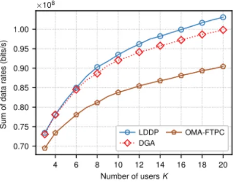
4 6 8 10 12 14 16 18 20 Number of users K 0.70 0.75 0.80 0.85 0.90 0.95 1.00 S u m o f d a ta ra te s (b it s /s ) ×108 LDDP DGA OMA-FTPC
Fig. 2. Sum of data rates vs. different number of users, M = 2
4 6 8 10 12 14 16 18 20 Number of users K 0.70 0.75 0.80 0.85 0.90 0.95 1.00 1.05 S u m o f d a ta ra te s (b it s /s ) ×108 LDDP DGA OMA-FTPC
Fig. 3. Sum of data rates vs. different number of users, M = 3
4 6 8 10 12 14 16 18 20 Number of users K 1.00% 2.00% 3.00% 4.00% 5.00% P e rf o rm a n c e lo s s DGA DPGA DIWA NOMA-SIWA-FTPC
Fig. 4. Performance loss vs. different number of users, M = 2
4 6 8 10 12 14 16 18 20 Number of users K 0.00% 0.25% 0.50% 0.75% 1.00% 1.25% 1.50% 1.75% P e rf o rm a n c e lo s s DGA DPGA DIWA NOMA-SIWA-FTPC
2 3 4 5 6 Number of multiplexed users M 8.48 8.50 8.52 8.54 8.56 S u m o f d a ta ra te s (b it s /s ) ×107 LDDP DGA DPGA DIWA NOMA-SIWA-FTPC
Fig. 6. Sum of data rates vs. different number of multiplexed users
three-step method and the performance in OMA system given by OMA-FTPC. Since projected gradient descent algorithm (Algorithm 1) achieves the optimal solution to power control problem (5), in Fig. 2 and Fig. 3, we choose to compare its sum-rate performance applied in the three-step algorithm (i.e., DGA according to our aforementioned definition) to that of LDDP and OMA-FTPC with different number of users. The number of multiplexed users M of Fig. 2 and Fig. 3 is set to 2 and 3, respectively. This setting is based on an implementation point of view, i.e., reducing the receiver complexity and error propagation due to SIC [40].
In Fig. 2, it can be seen that the sum of data rates of each scheme increases with the number of users K. For any given
K, LDDP has the best performance among the three schemes.
Nevertheless, DGA achieves comparable sum of data rates to that of LDDP, see for example, when K = 20 and M = 2, the proposed DGA has a performance loss of only 3.14% when compared with LDDP. In addition, OMA-FTPC has the worst system performance among all. Similar conclusions can be drawn from Fig. 3. It is worth mentioning that the proposed scheme becomes more efficient with the increasing of M . For example, when K = 20 and M = 3, the performance loss of DGA when compared to LDDP is reduced to 1.71%.
In Fig. 4 and Fig. 5, we compare the sum of data rates performance of the three-step scheme under DGA, DPGA, DIWA, and NOMA-SIWA-FTPC. The x-axis indicates the number of users, while the y-axis represents the sum-rate performance loss compared to that of LDDP, which is defined as follows:
Rsum(LLDP )− Rsum
Rsum(LLDP )
, (45)
where Rsum(LLDP ) and Rsum refer to the solutions of LDDP and the three-step algorithm, respectively.
Fig. 4 shows the performance loss versus different number of users K of the four proposed schemes, where M = 2. It can be seen that, for fixed K, DGA has the smallest performance loss among these four schemes. Meanwhile, DIWA has a similar performance to that of DPGA. In addition, for any given K, NOMA-SIWA-FTPC has the largest performance loss among all.
Fig. 5 represents the performance loss of our proposed resource allocation strategies when compared with LDDP where the number of multiplexed users is assumed to be 3. The similar conclusions can be achieved to the scenario where 2 users are multiplexed on each subcarrier (Fig. 4), which are
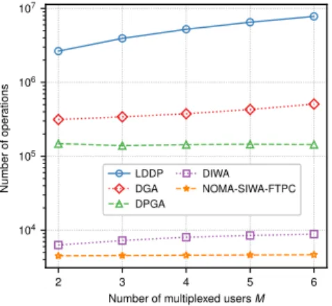
4 6 8 10 12 14 16 18 20 Number of users K 102 103 104 105 106 107 108 N u m b e r o f o p e ra ti o n s LDDP DGA DPGA DIWA NOMA-SIWA-FTPC OMA-FTPC
Fig. 7. Number of operations vs. different number of users, M = 2
4 6 8 10 12 14 16 18 20 Number of users K 102 103 104 105 106 107 108 109 N u m b e r o f o p e ra ti o n s LDDP DGA DPGA DIWA NOMA-SIWA-FTPC OMA-FTPC
Fig. 8. Number of operations vs. different number of users, M = 3
omitted here.
Fig. 6 depicts the sum of data rates of LDDP and our proposed resource allocation algorithms versus the number of multiplexed users M , in which the number of users K is assumed to be 6. It can be seen that with the increasing of M , the performance gap between LDDP and our proposed schemes decreases. For example, when M = 4, the proposed DGA and SIWA have almost the same performance to that of LDDP, i.e., a performance loss of approximately 0.0016% and 0.0074%, respectively, while DPGA stagnates at 0.036% and NOMA-SIWA-FTPC has a performance loss of 0.37%.
C. Number of Operations
Fig. 7 to Fig. 9 show the number of operations required by the different schemes. For each scheme, we count the number of additions, multiplications, and comparisons used, which reflects the time complexity, as an estimation.
In Fig. 7 and Fig. 8, the number of multiplexed users M is fixed to 2 and 3, respectively. We see that except OMA-FTPC, the number of operations for each scheme increases with the increasing number of users, K. For any given K, DGA has the highest computational complexity among the proposed algorithms (DGA, DPGA, DIWA, NOMA-SIWA-FTPC). OMA-FTPC requires the fewest operations of all. In addition, the proposed DIWA uses approximately the same number of operations as NOMA-SIWA-FTPC and slightly more operations than OMA-FTPC but much less operations
2 3 4 5 6 Number of multiplexed users M 104 105 106 10 N u m b e r o f o p e ra ti o n s LDDP DGA DPGA DIWA NOMA-SIWA-FTPC
Fig. 9. Number of operations vs. different number of multiplexed users
5 10 15 20 Number of users K 0.80 0.85 0.90 0.95 1.00 1.05 S u m o f d a ta ra te s (b it s /s ) ×108 LDDP, J = 200 LDDP, J = 10K LDDP, J = 50 LDDP, J = 20 LDDP, J = 10 DGA
Fig. 10. Sum of data rates for different values of J , M = 3
than DPGA and DGA. In any case, all of the proposed schemes are much more time efficient than LDDP especially when the number of users is large. For example, when K = 20 and M = 2, the number of operations required by DIWA, DPGA and DGA is less than 0.1%, 0.2%, and 0.27% of that required by LDDP, respectively. Besides, when K = 20 and
M = 3, the needed operations of DIWA, DPGA and DGA
is around 0.01%, 0.07%, and 0.1% of that needed by LDDP, respectively.
Fig. 9 compares the number of operations required under different number of multiplexed users M with fixed number of users K = 6. We can see that for any given M , the number of operations of LDDP is the highest of all. In addition, with the increasing of M , the computational complexity of LDDP has the fastest growth rate among all the schemes.
D. Impact of the Power Levels J on LDDP’s Performance
We show in this subsection how the sum-rate and com-plexity of LDDP depends on the number of power levels
J and the system’s parameters. We present in Fig. 10 and
Fig. 11 the sum-rate and number of operations of LDDP under different number of power levels J = 10, 20, 50, 200 and 10K, and compare them to the performance of DGA. As expected from [25], when J increases, the sum-rate of LDDP increases until reaching the optimal, while the computational complexity increases in O(CN M KJ2). The number of power levels considered here is always greater than 10, otherwise
5 10 15 20 Number of users K 105 106 107 108 N u m b e r o f o p e ra ti o n s LDDP, J = 200 LDDP, J = 10K LDDP, J = 50 LDDP, J = 20 LDDP, J = 10 DGA
Fig. 11. Number of operations for different values of J , M = 3
LDDP would not have enough discrete power steps to serve all N = 10 subcarriers.
We observe in Fig. 10 that LDDP’s sum-rate for J = 200 and J = 10K are very close, i.e. they have less than 0.01% of difference for any number of users. Hence, LDDP’s sum-rate does not improve significantly by further increasing J over 10K. Furthermore, the sum-rate is reduced significantly as J decreases. This justifies the choice of LDDP with 10 power steps per user, i.e. J = 10K, as a benchmark near-optimal scheme in our simulations. Note that this value only holds for the system’s parameters described in Table II. We discuss below how J can be set in other systems depending on N , K and M .
As the number of resource increases (subcarriers N , users
K, M , etc.), J should also increase in order to achieve similar
gain in the joint subcarrier and power allocation. The idea is that each allocated user should have enough power steps to optimize the allocation of their individual power budget ¯pk among the subcarriers in LDDP. Given that the number of allocated user is at most min{K, MN}, we choose empirically
J = O(min{K, MN}), which achieves good performance by
simulation. For example, we choose J = 10K in Fig. 10, since K < M N = 30.
In Fig. 11, all LDDP schemes have higher complexity than DGA. Among these schemes, only LDDP with J = 50, 200, 10K achieve better sum-rate performance than DGA. The performance gains compared to DGA, for K = 20, are re-spectively 1.04% and 1.74% for J = 50 and J = 10K = 200, while the increase in complexity are approximately 100 and 1000 folds. Moreover, DGA outperforms both LDDP with
J = 10 and J = 20 in terms of higher sum-rate and lower
complexity. For K = 20, the performance loss of LDDP with
J = 10 and J = 20 compared to DGA are respectively 3.20%
and 1.54%.
In summary, DGA has close to the best LDDP’s sum-rate, while requiring less computational complexity. The latter statement can be explained by comparing the asymptotic complexity of LDDP iteration O(N M KJ2) and DGA it-eration O(N K2). As discussed previously, we can assume
J = O(min{K, MN}). If K ≤ MN (which is the case
considered in our simulations), LDDP iteration’s complexity can be written as O(N M K3). In this case, DGA requires M K times less operations than LDDP, which explains the results
4 6 8 10 12 14 16 18 20 Number of users K 0.2 0.3 0.4 0.5 0.6 0.7 0.8 J a in ’s fa ir n e s s
DGA proportional power constraints DGA equal power constraints
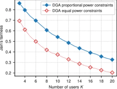
Fig. 12. Fairness index vs. different number of users, M = 2
4 6 8 10 12 14 16 18 20 Number of users K 0.75 0.80 0.85 0.90 0.95 1.00 S u m o f d a ta ra te s (b it s /s ) ×108
DGA proportional power constraints DGA equal power constraints
Fig. 13. Sum of data rates vs. different number of users, M = 2
shown in Fig. 7, 8, 9 and Fig. 11. Otherwise if K > M N , then LDDP iteration’s complexity becomes O(N3M3K). This
complexity is in practice higher than DGA’s iteration complex-ity. Indeed, let’s consider a 3GPP-LTE use case [44] with a bandwidth of 10 MHz divided in N = 50 resource blocks, and let M = 2, DGA remains advantageous in terms of computational complexity as long as K < N2M3, i.e. up to 20, 000 connected users.
E. Fairness Performance
As stated in Section II, the fairness among users can be obtained via adjusting the power constraint of individual user. We adopt Jain’s fairness index [45] to show this performance, which is defined as (
∑K k=1Rk)2
K∑K k=1R2k
. Fig. 12 depicts the fairness performance of the proposed scheme1 under different user
power constraint strategies where the number of multiplexed user on each subcarrier is set to 2. Specifically, under DGA equal power constraints, each user has the same maximum power budget, i.e., ¯pk = Ptotal/K, where k∈ K. Meanwhile, in DGA proportional power constraints, the power budget of user k, ¯pk, is given as follows:
¯ pk= (∑n∈Ngn k)−1 ∑ j∈K( ∑ n∈Ng n j)−1 Ptotal, k∈ K. (46) From Fig. 12 we see that, given the number of users, DGA under proportional power constraints has higher fairness index than that of DGA with equal power constraint. For example,
1For expression simplicity, we choose DGA as an example to demonstrate
the fairness performance. Similar conclusions can be obtained for the other proposed resource allocation schemes.
4 8 12 16 20 Number of users K 0.1 0.2 0.3 0.4 0.5 0.6 0.7 0.8 0.9 1.0 J a in ’s fa ir n e s s LDDP
DGA proportional power constraints DGA equal power constraints
Fig. 14. Fairness index over a scheduling frame, M = 2
4 8 12 16 20 Number of users K 0.70 0.75 0.80 0.85 0.90 0.95 1.00 S u m o f d a ta ra te s (b it s /s ) ×108 LDDP
DGA proportional power constraints DGA equal power constraints
Fig. 15. Sum of data rates over a scheduling frame, M = 2
when K = 20, DGA with proportional power constraints improves Jain’s fairness index by 60% when compared to that of equal power constraint scheme.
Fig. 13 is applied to illustrate the sum rate performance of DGA under different power constraint methods where two users are multiplexed on each subcarrier. For each value of K, DGA under equal power budget has better sum rate performance than DGA with proportional power constraints since the latter scheme assigns more power to users with weak channel conditions, resulting in sum rate performance degradation, e.g., when K = 20, DGA with proportional power budget has 7.3% sum rate loss when compared to that of equal power budget.
F. Fairness Performance over a Scheduling Frame
In this subsection, we compare the fairness performance of DGA with proportional power constraint to LDDP with weighting factor proposed in [25]. In the same way as in [25], we consider a scheduling frame of T = 20 times slots. The channel state information is collected at the beginning of the frame. Let Rk(t) be user k’s achievable data rate at time slot
t∈ {1, . . . , T }. We define user k’s average rate prior to time
slot t as follows: ¯ Rk(t) = ( 1− 1 T ) ¯ Rk(t− 1) + 1 TRk(t). (47)
At each time t, LDDP is applied to optimize the weighted sum-rate ∑kwk(t)Rk(t), where the weight wk(t) of each user k