Série Scientifique
Scientific Series
99s-12
Using Employee Level
Data in a Firm Level
Econometric Study
Jacques Mairesse, Nathalie Greenan
Montréal Mars 1999
CIRANO
Le CIRANO est un organisme sans but lucratif constitué en vertu de la Loi des compagnies du Québec. Le financement de son infrastructure et de ses activités de recherche provient des cotisations de ses organisations-membres, d=une subvention d=infrastructure du ministère de l=Industrie, du Commerce, de la Science et de la Technologie, de même que des subventions et mandats obtenus par ses équipes de recherche. La Série Scientifique est la réalisation d=une des missions que s=est données le CIRANO, soit de développer l=analyse scientifique des organisations et des comportements stratégiques.
CIRANO is a private non-profit organization incorporated under the Québec Companies Act. Its infrastructure and research activities are funded through fees paid by member organizations, an infrastructure grant from the Ministère de l=Industrie, du Commerce, de la Science et de la Technologie, and grants and research mandates obtained by its research teams. The Scientific Series fulfils one of the missions of CIRANO: to develop the scientific analysis of organizations and strategic behaviour.
Les organisations-partenaires / The Partner Organizations $École des Hautes Études Commerciales
$École Polytechnique $Université Concordia $Université de Montréal $Université du Québec à Montréal $Université Laval
$Université McGill $MEQ
$MICST
$Alcan Aluminium Ltée $Banque Nationale du Canada $Bell Canada
$Développement des ressources humaines Canada (DRHC) $Egis
$Fédération des caisses populaires Desjardins de Montréal et de l=Ouest-du-Québec $Hydro-Québec
$Imasco $Industrie Canada $Microcell Labs inc.
$Raymond Chabot Grant Thornton $Téléglobe Canada
$Ville de Montréal
© 1999 Jacques Mairesse et Nathalie Greenan. Tous droits réservés. All rights reserved. Reproduction partielle permise avec citation du document source, incluant la notice ©.
Short sections may be quoted without explicit permission, provided that full credit, including © notice, is given to the source.
ISSN 1198-8177
Ce document est publié dans l=intention de rendre accessibles les résultats préliminaires de la recherche effectuée au CIRANO, afin de susciter des échanges et des suggestions. Les idées et les opinions émises sont sous l=unique responsabilité des auteurs, et ne représentent pas nécessairement les positions du CIRANO ou de ses partenaires.
This paper presents preliminary research carried out at CIRANO and aims to encourage discussion and comment. The observations and viewpoints expressed are the sole responsibility of the authors. They do not necessarily represent positions of CIRANO or its partners.
Using Employee Level Data
in a Firm Level Econometric Study
*
Jacques Mairesse
H, Nathalie Greenan
IRésumé / Abstract
* Corresponding Author: Jacques Mairesse, INSEE–CREST, 15 boulevard Gabriel Peri, 92245 Malakoff
Cedex, France. e-mail: [email protected]
We are grateful to Zvi Griliches for discussion and for referring us to Fuller's 1987 book, and to Bruno Crepon, Bronwyn Hall and a referee for useful comments. We are also thankful to the Statistical Office of the Ministère du travail and to INSEE for providing us with the employee survey and firm data bases which are being matched. The first author has also benefitted from the hospitality of CIRANO and IFS (London) while revising the paper.
† INSEE–CREST (Paris) and NBER (Cambridge) ‡ Centre d'étude de l'emploi (Noisy-le-Grand)
Dans cet article, nous mettons en avant et argumentons l'idée suivant laquelle les études économétriques sur les entreprises peuvent être efficacement et substantiellement enrichies à l'aide d'informations obtenues aupres de leurs employés, même si seuls quelques-uns par entreprise, deux ou trois par exemple, sont interrogés. Alors même que les variables mesurées à partir des réponses d'un très petit nombre d'employés par entreprise sont sujettes à d'importantes erreurs d'échantillonnage, elles peuvent être utilement incorporées dans un modèle économétrique spécifié au niveau de l'entreprise. Dans une première partie de l'article, nous montrons, pour un modèle de régression linéaire, que les biais d'estimation sur les paramètres d'intérêt qui proviennent de telles erreurs d'échantillonnage, peuvent être corrigés, si on dispose au minimum d'un sous-échantillon (suffisamment grand) d'entreprises où on a pu interroger, au moins, deux employés choisis au hasard. Dans la deuxième partie de l'article, nous considérons, à titre d'exemple, l'estimation de la relation entre le salaire moyen des entreprises (connu directement à partir de leurs données comptables) et la proportion de leurs employés de sexe féminin, telle qu'elle peut être elle-même estimée à partir du sexe de un, deux ou trois salariés choisis au hasard par entreprise. En guise de test, nous comparons les estimations établies sur cette base avec celles obtenues sur la base de la « vraie » proportion d'employés de sexe féminin (c'est à dire la proportion pour tous les employés), que nous pouvons connaitre aussi, par ailleurs, directement auprès des entreprises. Cette analyse est effectuée sur deux échantillons appariés « entreprises-salariés », relatifs à environ 2500 entreprises, en 1987 et 1993, pour l'industrie et les services en France, entreprises où un, deux et trois employés ont été interrogés pour respectivement 75 %, 15 % et 10 % d'entre elles.
In this paper, we make the general point that econometric studies of the firm can be effectively and substantially enriched by using information collected from employees, even if only a few of them are surveyed per firm. Though variables measured on the basis of the answers of very few employees per firm are
subject to very important sampling errors, they can be usefully included in a model specified at the firm level. In the first part of the paper, we show that in estimating parameters of interest in a regression model of the firm, the biases arising from the sampling errors in the employee based variables can be assessed, as long as we have a large enough sub-sample of firms with at least two or with more (randomly chosen) surveyed employees. As an illustration in the second part of the paper, we consider the estimation of the relationship between the firm average wage (directly obtained from the firm accounts) and estimates of the proportion of female workers based on the gender of one, two or three surveyed employees per firm. As a test, we compare the estimates that we find in this way with those using the "true" proportion of female workers (i.e., based on all the employees), which we could also directly obtain at the firm level from a firm survey. The analysis is performed on two linked employer-employee samples of about 2500 firms in the French manufacturing and services industries in 1987 and 1993, with one, two or three surveyed employees per firm (for respectively 75%, 15% and 10% of the firms).
Mots Clés : Données appariées entreprises-salariés, modèles à erreurs sur les variables, pseudo-panels, écarts salariaux hommes-femmes. Keywords : Linked employer-employee data, errors in variables,
pseudo-panel, wage gender differentials JEL : O33
1
1. Introduction
One of the main reasons explaining the rapid development of micro-econometric analyses over the last twenty years, and in particular the rise of panel data econometrics, is a negative one: the discontent with the small number of observations in annual (or even quarterly) aggregate data, the high degree of collinearity of macro-variables, and hence the poor precision of estimates and lack of power of statistical tests. Over the years, however, applied econometricians have become increasingly aware that large sample sizes are not enough, even if crucial for the use of some of the more recent sophisticated techniques. They have discovered (or rediscovered) that the quality of the measurement of the variables is an important factor, but also that the sheer existence or availability of certain variables is often an even more critical concern, setting drastic limits on the questions that can be considered and the ways in which they can be investigated. To push away such limits and go beyond what can be done with the more traditional sources of information, such as the firm accounts, population census or consumption and employment surveys, empirical economists are tending to put more efforts in conceiving and constructing new data bases of their own, or in helping official statistical offices to do so. A prominent example of such promising evolution is the recent very rapid development of employee-employer matched data. Labor economists are the driving force in this construction, trying mainly to complement the available information on the individual characteristics and wages of workers, with information on the firms and professional environment in which they work. What we propose here is in a sense the dual attitude. In this paper, we make the general point that using information collected from employees can effectively and substantially enrich econometric studies of the firm. More specifically, we try to make the case that this is so even if only very few employees are surveyed per firm, provided they are randomly chosen in the firm. Though variables measured on the basis of very few employees per firm are subject to very important sampling errors, they can be usefully included in a model specified at the firm level.
The variables that can be estimated on the basis of the answers of the employees surveyed in the firm may be of very different types. They may be quantitative and continuous, as we assume in the errors in variables regression framework presented in this paper. But very frequently they will also be in the nature of a proportion based on the employee ’yes’ or ’no’ answer to a qualitative question, as in the application considered in the paper, or more
2
generally in the nature of a vector of proportions based on the employee assignment to given categories. They may correspond to some objective and simple enough characteristics, such as the age of the interviewed employee, or the number of years of job experience, or the sex, or the fact that he or she uses a computer at work, etc.. But they may also be related to more subjective features, possibly concerning the firm itself as a whole that will be defined from employee’s answers to a set of questions. Examples of such features range from the autonomy at work and on the job satisfaction of employees to the managerial ability of executives, the organizational flexibility of the firm or its social climate, etc.. Variables of this sort raise problematic definitional issues but they could be of particular interest in many analyses of firm behavior and performance; being difficult, both conceptually and practically, to comprehend and measure directly at the firm level, they have to be constructed from employee surveys, and one will have to analyze them in an error in variables framework similar to the one presented here.
In the second section of the paper, we show that in estimating parameters of interest in a regression model of the firm, the biases arising from the sampling errors in the employee based variables can be assessed, as long as we have a large enough sub-sample of firms with at least two or with more (randomly chosen) surveyed employees.
As an illustrative exercise in the third section of the paper, we consider the estimation of the relationship between the firm average wage (directly obtained from the firm accounts), and estimates of the proportion of female workers based on the gender of one, two or three surveyed employees per firm. For the sake of our demonstration, we also compare the estimates that we find in this way with those using the "true" proportion of female workers, (i.e., based on all the employees), which we could also directly obtain at the firm level from a firm survey. The analysis is performed on two linked employer-employee samples of about 2500 firms in the French manufacturing and services industries in 1987 and 1993, with one, two or three surveyed employees per firm, for respectively 75%, 15% and 10% of the firms.
In the conclusion, we stress again the usefulness of the method in showing that it can also be applied in the context of firm panel data, and end with a few words of advice on how to proceed in matching an employee survey to firm data.
3
2. Assessing the biases from using employee level variables in
the estimation of a firm level model
2.1 - A simple sampling errors in variables model
We consider the following simple regression model specified at the firm level: yi = α xi* + εi
for i = 1 to N, where i is the subscript for the i th firm in the sample of N firms considered, where yi is "explained" by xi* and α is the parameter of
interest. As usual εi denotes the disturbance term in the regression,
summarizing all sources of "errors", which we assume to be uncorrelated with xi*.1 However, unlike the dependent variable yi , the explanatory variable xi* is
not known at the firm level, either simply because it is "unobserved" or more deeply because it should be thought of as an "unobservable" latent variable: that is either a variable which is not recorded in the firm information available for the analysis, but could be in principle measured and included in future investigation, or a variable which is too costly or too problematic, or both, to define and directly measure at the firm level.
The "true variable" xi* can however be estimated or proxied by the firm level
empirical average xi of an employee survey based variable. If there is ni
surveyed employees in the i th firm and if h denotes the h th surveyed employee among the ni surveyed employees, we have
xi = ( h ni =
∑
1 xih ) / niwhere the variable xih directly corresponds to the answer of the surveyed
employee h in the firm i to an appropriate question or can be constructed from his or her answers to a relevant set of questions, and where the summation is over all the ni surveyed employees in firm i.
2
As we already stress in the
1
We also assume that ε is i.i.d., with E(εi) = 0 and Var(εi) = σε , and we delete the constant in
the regression for simplification without real loss of generality.
2
For simplicity and since our model of interest is specified at the firm level, we use the notation xi rather than the usual notation xi. (where the dot subscript indicates over which index the mean
of xih is computed). Note also that we simply use xi rather than the more precise xi or xi (with the
overbar or the overhat reminding that it is an estimate over the random sample of the ni surveyed
4
introduction, the scope of firm level variables x which can be constructed from employee level variables is extremely large; evidently, however, all firm variables do not fall in this category. In particular it should clear that we do not need to assume that this is the case for the dependent variable y (or for other variables than x in the equation), although it will be in our application in the next section.3
Depending on the number ni of surveyed employees per firm, the observed xi
is more or less affected by sampling errors, and using it to approximate the "true" xi* in the model will cause the ordinary least squares estimator of α to
be more or less severely biased. It is easy to see that we are in a classical case of random errors in variables, but fortunately in a case where we can estimate the error variance and hence compute a corrected least squares estimator, which will be consistent.
Assuming first that the ni surveyed employees are randomly drawn among all
the employees of firm i, then xi is a consistent (and unbiased) estimate of the
"true" xi *
, and its variance is decreasing with ni . This assumption will
evidently be fulfilled by construction, in the case where the employee data set is obtained by choosing at random the surveyed employees in each of the firm of the firm sample to be considered. But it is also fulfilled in the more usual case where the employee and the firm data sets to be linked are independently constructed, and where the persons surveyed in the employee sample are randomly chosen in the total population or labor force. This is the case of our application in the next section.4
3
In our application all the firm variables can be viewed as employee variables aggregates, y being the log of the average firm wage per employee (not though the average log wage), x the proportion of female employees and the control variables z the proportions of employees according to three types of skills (or occupations). In fact the wage equation we estimate, although we consider it at the firm level, can be simply viewed as resulting of the agregation of underlying employee level wage equations (see for example Haegeland and Klette in this volume for an explicit derivation). However, this of course does not need to be. We could have considered for example a productivity equation, where the production function is directly defined as a firm (or plant) level relationship and where the productivity variable measured by output or value added per employee or the capital variable by gross book values or insurance values of fixed assets per employee cannot be really considered as employee level agregates (see again Haegeland and Klette in this volume, who estimate gender, education and experience effects for both wage and productivity equations at the plant level, or Greenan and Mairesse, 1996, who do the same at the firm level for computer use impacts).
4
Note that in this case the number of surveyed employee per firm ni will tend to be larger with
5
Assuming further that the individual answers xih of the surveyed employees in
firm i are independently distributed, the variance of xi is in fact just that of xih
divided by ni .5 More precisely, we can write:
xih = xi* + eih
with:
E(xih|i) = xi* , or E(eih|i) = 0 , and Var(xih|i) = Var(eih|i) = σi2
and hence:
xi = xi* + ei
with:
E(xi|i) = xi *
, or E(ei|i) = 0 , and Var(xi|i) = Var(ei|i) = σi 2
/ ni
where eih is the sampling error on xih of variance σi2, and where ei is the
sampling error on xi of variance σi2 / ni , that is by definition:
ei = ( h ni =
∑
1eih ) / ni , and σi2 = Var(xih|i ) = E[(
h ni =
∑
1 (xi h -xi )2 / (ni - 1)) |i]It is important to note that σi 2
cannot be estimated for ni = 1. Note also that
when needs be, in what follows, we will simply assume that σi2 is independent
of the xi’s and equal for all firms (i.e., σi2 = σ2).6
Considering next that the sample of firms itself arises at random from an underlying (large) population of firms, we can see that the sampling errors ei’s
are uncorrelated across firms with the true values of the xi’s. More precisely,
we can write:
E(ei ) = E[E(ei|i)] = 0 , and Cov(ei xi * ) = E(ei xi * ) = E[E(ei xi *| i)] = 0 and hence:
5 This will be the case if x is a continuously distributed variable as we assumed in this section.
For a discrete variable, this will also be the case if in principle the surveyed employees are randomly drawn in the firm with remise, or if in practice the total number of employees in this firm is not too small. This is true for our application in the next section, where we consider a sample of firms with twenty or more employees. This should also be true, however, for firms of about 10 employees. For firms of a smaller size, one will have to make appropriate corrections in deriving the variance of xi from that of xih .
6
This assumption can be relaxed in different ways. It is not made in our application in the next section, where xi is the estimated mean pi of a binomial variable B(pi*; ni ) and where σi2 is thus
6
E(xi ) = E(xi*) , and Var(xi ) = Var(xi*) + Var(ei )
where Var(xi ) and Var(ei ) are respectively the (across firms) variance of the
estimated xi’s and that of the sampling errors ei’s, and where Var(xi*) is the
corresponding "true" variance. Note that in the usual terminology of the analysis of the variance, Var(xi ), Var(ei ) and Var(xi*) are simply the
"between firm" variance of the "firm-employee" variables xih , eih and xih*
respectively.7
Considering finally the approximate equation where one uses the estimated xi
instead of the "true" ones xi *
, we have:
yi = α xi + vi with vi = εi - α ei
and see that we are in the pure classical textbook case of a random uncorrelated errors in variables model.
2.2 - Correcting the least squares estimator
We know (and can easily verify) that the ordinary least squares (OLS) estimator
α
ˆ
of the parameter of interest α, in the approximate equation with the measured xi’s, is biased downward in proportion to λ, where λ is the shareof the sampling error variance of the xi's in their measured variance, or
equivalently (1- λ) is the share of the true variance in the measured variance. More precisely, we have:
plim(
α
ˆ
) = Cov(xi yi ) / Var(xi ) = (1- λ) αwith
λ = Var(ei ) / Var(xi ) = Var(ei ) / [Var(xi * ) + Var(ei )] or (1- λ) = Var(xi * ) / Var(xi ) = Var(xi * ) / [Var(xi * ) + Var(ei )
The important point here is that as long as we have at least a (large enough) sub-sample with more than one employee surveyed per firm, we can estimate
7
Note also that while expectations or variances, such as E(xi|i) and Var(xi|i), are only taken
over the random sample of surveyed employees in firm i , expectations and variances like E(zi )
and Var(zi ) are also taken over the (random) sample of firms. Again for the sake of easiness and
in the absence of ambiguity in the present context, we do not use the more precise notations Ei(zi)
7
the error and true variances, and hence we can simply obtain a consistent estimate of α.
Consider first a sub-sample with a constant number n of surveyed employees per firm (ni = n), we can write:
Var(ei ) = E[Var(ei|i)] + Var[E(ei|i)] = E[Var(ei|i)] = E(σi 2
)/ n = σ2/n and
λ = σ2 / [n Var(xi )] = σ2 / [n Var(xi* ) + σ2 ]
Note that σ2 (equal σi2 ) and Var(xi ) can be respectively viewed as the
sub-sample "within firm" (across employee) variance and the sub-sub-sample "between firm" variance of the individual employee variable xih .8
It is clear from these formulas that the relative bias λ decreases with n. For example, if we suppose that Var(xi
*
) = σ2 , we have λ equals one half, one third or one fourth for the sub-samples with respectively one, two or three surveyed employees. If indeed we consider separately such sub-samples, as we shall do in our application in the next section, we should be able to check that the biased least squares estimates of our parameter of interest tend to be greater (in absolute value) in sub-samples with two surveyed employees than in those with only one, and in those with three surveyed employees than in those with two.9 Although these formulas apply for all n (including n=1), it must be remembered that σ2 can only be estimated in the sub-samples with n larger than one.
Considering next the full sample, we can immediately generalize the above formulas by combining them for all the sub-samples with two or more surveyed employees per firm. This amounts to simply taking for σ2 the overall within firm (across employee) variance and for n the weighted harmonic mean of the numbers of surveyed employees per firm, for all the firms with more than one surveyed employee.
8 Note that the expression n Var(x
i ) =n Var(xi* ) + σ2 can also be seen as the between -within
decomposition of the total variance in the analysis of variance model xih = xi* + eih .
9 Note that one could in principle retrieve consistent estimates of λ and α from such relations
between the OLS estimated α and the observed variances of the measured x‘s for the different sub-samples with a constant number of surveyed employees per firm, that is just using the fact that of being able to identify these sub-samples. It is likely, however, that these estimates will be much more inaccurate than the estimates we considered here, which are also using the within firm across employees information in these sub-samples to estimate σ2 , and hence λ.
8
More precisely, let us suppose that the full sample is made of S sub-samples with different numbers of surveyed employees per firm, the sth sub-sample consisting of the Ns firms with s surveyed employees per firm, the weighted
harmonic mean n is such as:
(1/n) = s S =
∑
2 Πs (1/ns) with Πs = Ns / [ s S =∑
2 Ns ]where Πs is the proportion of firms with s more than one surveyed employees
among all the firms with more than one surveyed employees.
Using now this value for n , the previous formulas apply, and we can write: Var(ei ) = (σ2 / n)
and
Var(xi* ) = Var(xi ) - Var(ei)
where σ2 and Var(xi), that we can also denote σw2 and σb2 from now on, are
respectively the overall (across employee) within firm and overall between firm variances of the individual employee variable xih.
Finally one obtains a consistent corrected least squares (CLS) estimator
α
~
of the parameter of interest α by substituting in the formula of the OLS estimatorα
ˆ
the estimated true variance for the measured one, that is:α
~
= [Vˆ
ar(xi* )]-1 [
Cˆ
ov(xi yi )]or
α
~
= [Vˆ
ar(xi ) -
Vˆ
ar(ei )]-1 [Cˆ
ov(xi yi )] = [sb2 - (sw2 / n)]-1 [Cˆ
ov(xi yi )]Applying this corrected estimator is in practice simple enough. To do so, we only need to obtain a consistent estimate of the error variance, and hence of the true variance of the xi’s. For this we can rely on estimating the (across
employee) within firm variance σw2 , which in turn is possible if we have at
9 2.3 - Remarks and extension
It is worthwhile to make a number of remarks on the above corrected least squares (CLS) estimator, and in particular that it easily generalizes to the case of the multivariate linear regression.
1) It is interesting first to note that the usual t-ratio test of significance of α, based on the ordinary least squares estimate
α
ˆ
and its estimated standard error, remains valid. Actually under the null hypothesis ofα = 0 , whatever the sampling errors, the OLS estimate
α
ˆ
is unbiased (i.e., E(α) = 0), and the distribution of the t-ratio is unaffected (following a Student’s t distribution in a small sample if the error in the equation is itself normal). Thus even if one has to use a variable which happens to be only based on the answers of one interviewed employee per firm, one can in principle find out whether this variable is significant or not as an explanatory variable.2) In the same vein, it is always possible to use an employee based variable as the right hand side variable to be explained in a firm level regression. This simply amounts to adding another source of (uncorrelated) error to the regression, and this is not per se a cause of bias of the OLS estimator, but will affect its precision, and possibly quite severely so.
3) One has to be aware, however, that in small samples the corrected estimator (as defined) is not always a proper estimator. This will be the case if the estimated error variance
Vˆ
ar(ei ) happens to be larger than the observedvariance
Vˆ
ar(xi ) , implying that a non positive estimateVˆ
ar(xi*) of the truevariance. Fuller (1987) proposes a partial adjusment technique to take care of this case, but it remains in practise much preferable when the estimated error variance is not a very large fraction of the observed variance.10
4) This last remark raises the problem of the precision of the corrected estimator
α
~
as compared to that of the OLS estimatorα
ˆ
. In terms of its formula, the corrected estimator can simply be viewed as an OLS estimator performed on the true equation, where one would be using the true10
Note that one must have in fact the following condition, which is more restrictive than
Vˆ
ar(ei ) <Vˆ
ar(xi ) :Vˆ
ar(εi ) =Vˆ
ar(yi -α
~
xi ) positive, that is10
variance Var(xi*) of the xi’s ( and since we have Cov(xi yi ) = Cov(xi*yi )). One
might thus expect the standard error of
α
~
to be larger than that of the corresponding (biased) least square estimateα
ˆ
because of its smaller denominator, equal to [Var(xi*)]1/2 instead of [Var(xi )]1/2 , and thereforesmaller by a factor of (1-λ )1/2.
This is in fact too simplistic. It is better, but also not quite right, to view the corrected estimator as an instrumental variable estimator where one would be using the true xi’s (if one knew them!) to instrument the measured xi’s (since
we also have Var(xi*) = Cov(xi*xi )). Thus another reason of why the standard
error of
α
~
is larger than that of its least squares counterpartα
ˆ
, is a larger estimated numerator (equal toVˆ
ar(vi ), the estimated variance of vi , theerror in the estimated equation, which by definition is minimum at the least squares estimation). Yet another reason will be the fact that the error variance Var(ei ) is not exactly known but is estimated with varying precision.
5) Actually the derivation of the standard error of the corrected estimator
α
~
is not too easy; and one has to use large sample theory to obtain its limiting distribution. The formula for the asymptotic variance ofα
~
(assuming normality of the sampling error ei and the error in the equation εi )is the following when the error variance
Vˆ
ar(ei ) is exactly (very precisely)known:
Vˆ
ar(α
~
) = (N-1)-1 [Vˆ
ar(xi*)]-2 [Vˆ
ar(xi )Vˆ
ar(vi ) +α
~
2Vˆ
ar(ei )Vˆ
ar(ei )]where the first term (N-1)-1 [
Vˆ
ar(xi*)]-2 [Vˆ
ar(xi )Vˆ
ar(vi )] is that of theinstrumental variable estimator as just suggested. When the error variance is estimated, the formula includes an additional third term (n)-1(N-1)-1 [
Vˆ
ar(xi*)]-2 [2α
~
2Vˆ
ar(ei )Vˆ
ar(ei )] , which decreases in proportion to n ,the average number of surveyed employee per firm (and can be neglected relatively to the other terms for large n ).11
11
The formula for a known error variance is the one given in Fuller 1987, theorem 1.2.1. See theorem .2.2.1 for a more general formula in the multiple regression case and when the error variance-covariance matrix is estimated in a situation as ours (that is independently from the variance-covariance matrix of the xi’s , but with a precision increasing with the size N of the
11
6) The results so far directly generalize to the multivariate linear regression model. This is the usual extension in the case of a regression with only one employee survey based variable xi and a number of firm level
measured variables zi . If we just want to focus on the coefficient of the
employee based variable x, we can rely on the so-called Frisch-Waugh procedure. That is first compute the residuals from the least squares projections of y (to be explained) and of x on the z (including the constant or a set of industry dummies), and then consider the simple regression between these residuals. We are back to the previous one explanatory variable specification, and the main change in the above formulas amounts to taking the partial or net variances of x and y, remaining unexplained by z, and the corresponding net covariance. One can see in particular that the relative bias λ can be much larger; it is now equal to the share of the unchanged error variance to the net observed variance of the xi’s, and is thus equal to the
previous λ in the equation without the additional control variables z, divided by (1-Rxz2), where Rxz2 is the multiple correlation coefficient of the regression
of x on the z.
7) The extension to the multivariate regression where there are several employee variables x is also straightforward. In practice one has first to compute an estimated variance-covariance matrix of the sampling errors in the (across employee) within firm dimension as before, and hence compute by difference with the observed variance-covariance matrix of the xi’s an estimate
of the true variance-covariance matrix; then one has simply to substitute the estimated true matrix for the observed one (in the overall variance-covariance matrix of the xi’s and z’s) to obtain a consistent corrected least squares
estimator of all the regression parameters.12.
8) Until now, we have assumed that σi2 = Var(xih|i) is independent of
the xi’s ; this is not true, however, in our application in the next section, where
the underlying process xih = pih is one of a zero-one binomial variable of
observed mean pi , with true mean pi* and variance σi2 = pi* (1-pi* ) for a given
firm i.13 Looking at this case of a binomial variable, we can see that in fact the
12
Note that in principle non-linear terms in the employee based x variables can be included in the regression. One must be must be aware, however, that non-linear errors in variables models raise important additional difficulties. See Chapter 3 in Fuller 1987; see also the note by Griliches and Ringstad, 1970.
13 Note that the problem is the same for a multinomial variable defined over a given set of
categories, corresponding to the extension from one binomial variable to a vector of interrelated binomial variables (i.e., one for each category).
12
only difference with what precedes is in the expressions of the error and true variances. We can write as before for the given firm i:
pi = pi*+ ei
with
E(pi |i) = pi* or E(ei |i) = 0
and
Var(pi|i) = Var(pi*|i) + Var(ei|i) = Var(pi*) + σi2/ni = Var(pi*) + pi*(1-pi*)/ni
from which we can directly derive that for the full sample of firms: Var(pi ) = Var(pi*) + Var(ei ) = Var(pi*) + E[pi*(1-pi*)/ni ]
or
Var(pi ) = Var(pi*) + [p*(1-p*) - Var(pi*)]/n = (n-1)Var(pi*)/n + p*(1-p*) /n
where p* denotes the full sample true mean, and where n is now defined as the weighted harmonic mean of the number of surveyed employees per firm for the full sample (and not only for the sub-samples with more than one surveyed employee as before). If there is only one surveyed employee per firm for all the firms in the sample, we see, as could be expected, that n=1 and Var(pi ) =
p*(1-p*), and hence the true variance Var(pi*) cannot be estimated. However, if
we have at least a sub-sample with more than one surveyed employee, n is larger than one and the true variance can simply be expressed as:
Var(pi* ) = [nVar(pi ) -p* (1-p* )] / (n-1)
and thus be consistently estimated on the basis of the full sample empirical variance
Vˆ
ar(pi ) and empirical meanp
(and the value of n).1414 We also verify, as before in the continuous variable case, that the difference between the
observed and true variances (i.e., the sampling errors variance) decreases in inverse proportion to n, when n increases.
13
3. Looking at the relation between the firm average wage and
the proportion of female employees
3.1 Variables, sample and sub-samples
Mainly as an illustration of our formal analysis, we consider the estimation of the relationship between the firm average wage (directly measured at the firm level from its current accounts) and the proportion of female employees which we can obtain at the firm level by matching an employee survey to the firm data bases maintained by the French statistical office INSEE. The survey is "l'enquête sur les Techniques et l'Organisation du Travail", known as TOTTO, which has been conducted in 1987 and in 1993, by the French "Ministère du Travail". TOTTO concerns a sample of individuals who have been working during the year, randomly drawn from the French labor force.15 TOTTO is a rich source of knowledge on the organisation of work and use of new technologies in the firm. It provides in particular unique information on computer use at work, which we have already matched to firm information in Greenan-Mairesse (1996), in an attempt to assess computer impacts on firm productivity.
We start here from the same matched samples as in this previous study, but for our present purpose we prefer to focus on the regressions of the firm average wage on the proportion of female workers, for which we expect moderately to strongly negative coefficients, depending on whether we (roughly) control for skill composition or we do not. The main reason for the choice of this example is that we can also know the average proportion of female employees among all the firm employees from a regular firm survey, "l'Enquête sur la Structure des Emplois"(ESE). The obvious interest is of course in allowing us to compare the estimates using the proportion MFEM of female workers in the firm, as estimated on the basis of the gender of the very few interviewed employees per firm in TOTTO, and the true proportion PFEM, or if not exactly true much more accurate proportion, as known by ESE. Also, we will be able to regress MFEM on PFEM, and thus directly verify whether a number
15 TOTTO is conducted as an occasional supplement to the regular survey on employment
"L'Enquête Emploi", which gives a selection probability of 1/1000 to each person in the French labor force, that is a sample of about 20 000. TOTTO proper concerns all the respondents who have been working during the year.
14
of implications of the classical random (non correlated) errors in variables framework, as developed in this paper, are indeed verified.
We linked the ESE firm surveys for 1987 and 1993 to the INSEE firm data sets, providing the usual accounting data from which we constructed the firm average wage variable LW (in logs) considered here.16 The ESE firm survey also allowed us to obtain the variables of the general skill composition of labor in the firm, which we use for controls in our firm wage regressions. We have estimated all the regressions with and without including the three skill variables PCA, PCP and PEA. These are defined respectively as the proportions in the firm total number of employees of the managers and executives in "administrative" occupations ("admistrateurs"), of the managers and executives in "productive" occupations ("ingénieurs"), and of the employees in admistrative subordinate positions or white-collars ("employés"). The remaining category, that of the blue-collars ("ouvriers"), is the left out category in the regressions; its proportion PEP adds up to 100% with PCA, PCP and PEA and is still the largest in many industries and overall. Quite obviously the main restriction on our final sample size results from the need to match the employee and firm data files. This we did by first tracing the SIREN identification number of the firm on the basis of its name and address as declared by the interviewed employees in TOTTO, and then using the SIREN to do the matching with the firm files. At both stages, important losses occur in the numbers of interviewed employees and firms that can in fact be linked. In the first stage this is in particular the case of self-employed persons; in the second one, this is mainly true for the interviewed employees working in the smaller firms. For that last reason, we excluded from our samples the firms with a total of less than 20 employees.17 In total, if we consider the population of the French firms of 20 and more employees in the Manufacturing and Services industries, any strong (non random) selectivity in the sample construction seems rather unlikely; we can be fairly confident that we obtain two random samples of firms in 1987 and 1993, and more importantly we can maintain that the interviewed employees are taken at random within these
16
These data sets come from SUSE ("Système Unifié de Statistiques d'Entreprises"), which combines the information of the firm annual surveys ("Enquêtes Annuelles d'Entreprises, EAE") and the firm fiscal declarations ("Déclarations de Bénéfices Industriels et Commerciaux, BIC").
17 We have also excluded public enterprises and-non profit organizations, and we have not
considered the Building, Construction, Energy, Transportation and Telecommunications industries, because of their specific features and/or because of the relatively small number of private firms concerned.
15
firms. Note in that respect that the probability that the individuals surveyed in TOTTO (since they are randomly drawn) would be employed in a given firm is increasing with its size; and indeed the median sizes of the firms in our sub-samples with one, two and three interviewed employees are respectively about 120, 330 and 730 employees. In all our regressions, we include three size dummies (two in addition to the constant), as well as seven industry dummies (six and the constant).
In the end, we have two samples of respectively 2563 and 2213 firms in 1987 and 1993, each consisting of three sub-samples of about respectively 75 percent of firms with only one interviewed employee, 15 percent with two, and the remaining 10 percent with three.18 To simplify matters, we have in fact abstracted from sub-samples with more interviewed employees per firm, by keeping only three interviewed employees chosen at random in the firms where there were four or more. To fully control for the actual differences between sub-samples (in size and industry composition and otherwise), and ascertain that the differences between the sub-samples estimates arise from the different number of interviewed employees, we have also considered what we call "restricted sub-samples" with one or two interviewed employees. These are constructed from the sub-samples with three interviewed employees by keeping only one or two of them at random, and similarly from the sub-samples with two interviewed by keeping only one of them at random.
The Table in the Appendix gives the average and standard deviations of the log wage LW, and of the estimated and true female proportion variables MFEM and PFEM, for the full samples, sub-samples with one, two or three interviewed employees (sub-samples 1,2 and 3 with respectively NS=1, 2 or 3), and the corresponding restricted sub-samples with one or two interviewed employees (sub-sample 2 with NS=1 and sub-sample 3 with NS=1 or 2). We see that the average wage is (in average) about the same across all sub-samples, increasing by nearly 30 percent in absolute terms between 1987 and 1993.19 Our estimated and true proportions of female workers MFEM and PFEM are also about the same across all different sub-samples, and stayed
18
Because of the new match with the ESE survey, the size of these samples is about 10% smaller (in number of firms) than that of our previous samples in Greenan and Mairesse, 1996.
19 Note that our average wage variable is really the average labor cost by employee for the firm,
including social security and other employee related charges paid by the firm. It amounts at the geometric mean (or roughly the median) to about 150 000 FF in 1987 and 200 000 FF in 1993 (or roughly 30 000 and 40 000 US $).
16
about 35 to 40 percent in the two years. But mainly we verify that the averages of the two variables are, as expected, very close, within 2 or 3 percent. We can also see, as expected too, that the standard deviations of the error-ridden MFEM are much larger than that of the true PFEM, from roughly the double in the sub-samples with one interviewed employee to 50 percent larger for those with three. Likewise we see that the standard deviations of MFEM are decreasing when we go from the sub-samples with one interviewed employee to the ones with two, and again, but less so, when we go from the ones with two to the ones with three.20 Much of what we find in what follows can in fact be traced back to these simple observations.
3.2 The ordinary least squares estimates
The ordinary least squares estimates of the gender coefficients in our firm average log wage regressions are given in Table 1, both for the estimated proportions MFEM of female workers and for the true proportions PFEM, and with and without controlling for skill composition differences. On the whole, the estimates agree remarkably well with what we expect.
First, nearly all of our estimates are significantly negative, but much smaller when we control for skill composition. The only non significant estimates we find are in fact obtained for the restricted sub-samples (of a relatively small size) with one interviewed employee per firm, when using the estimated MFEM (i.e., 0 or 1 on the basis of the gender of this interviewed employee). Second, the estimates using the estimated proportions MFEM are quite low relatively to the ones based on the true proportions PFEM, confirming that indeed they are severely biased downward due to sampling errors. For the full sample, for which these estimates are much more precise, the order of magnitude of the biases is roughly about 75 percent, which is what we could expect from the fact that the standard deviation of MFEM is twice that of PFEM.
Third, the estimates based on MFEM tend, as also expected, to increase when we go from the restricted sub-samples with one interviewed employee to the
20
One can also note that these standard deviations decrease by a factor of about (1.7)1/2 between the sub-samples with one and two interviewed employees, and of about (2.2)1/2 between those
with two and three. This is less than (2)1/2 and (3)1/2 which will the values to be found if the
differences in MFEM across firms only reflected sampling errors. There is thus room left for systematic true variance in MFEM: see Table 2 below.
Table 1: Ordinary Least Squares estimates of the coefficients of the estimated and true female proportions
MFEM PFEM MFEM PFEM
Without Controls for Skills With Controls for Skills
LW on 87 93 87 93 87 93 87 93 -0,14 -0,12 -0,48 -0,48 -0,09 -0,08 -0,39 -0,40 FULL SAMPLE (0.01) (0.01) (0.03) (0.03) (0.01) (0.01) (0.02) (0.02) -0,13 -0,12 -0,45 -0,47 -0,08 -0,09 -0,39 -0,41 SUBSAMPLE 1 NS = 1 (0.02) (0.02) (0.03) (0.03) (0.01) (0.01) (0.03) (0.03) -0,14 -0,04 -0,51 -0,49 -0,11 -0,01 -0,39 -0,37 NS = 1 (0.03) (0.04) (0.06) (0.08) (0.03) (0.03) (0.06) (0.06) -0,21 -0,11 idem idem -0,14 -0,05 idem idem
SUBSAMPLE 2 NS = 2 (0.04) (0.05) " " (0.04) (0.03) " " -0,08 -0,11 -0,63 -0,63 -0,03 -0,06 -0,36 -0,42 NS = 1 (0.03) (0.04) (0.08) (0.10) (0.02) (0.03) (0.06) (0.08) -0,14 -0,18 idem idem -0,06 -0,08 idem idem
NS = 2
(0.04) (0.05) " " (0.03) (0.04) " " -0,14 -0,21 idem idem -0,08 -0,10 idem idem
SUBSAMPLE 3
NS = 3
(0.05) (0.08) " " (0.03) (0.04) " "
MFEM: estimated female proportion; PFEM: "true" female proportion; and LW: log of the firm average wage All regressions include industry and size dummies.
The regressions in the two last columns also control for skill composition differences as measured by: PCA, PCP and PEA.
The number of firms N is: in the Full Sample: N=2563 in 1987 and N=2213 in 1993; in the First Subsample (with one interviewd employee): N=1882 in 1987 and N=1667 in 1993; in the Second Subsample (with two interviewd employees): N=363 in 1987 and N=314 in 1993; in the Third Subsample (with three intervied employees): N=318 in 1987 and N=232 in 1993.
idem means unchanged: PFEM being the true variable, the OLS estimates do not vary with the number of interviewed employees, for a given subsample.
18
corresponding ones with two and with three interviewed employees. This evidence, however, is rather weak because of the lack of precision of the estimates on the sub-samples with two and three interviewed employees, due to their relatively small size.21
3.3 The corrected least squares estimates
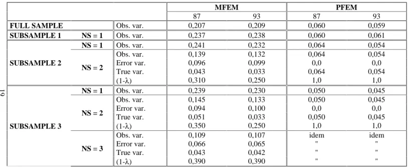
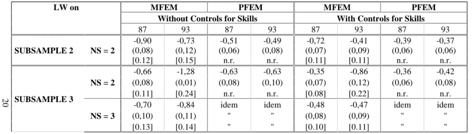
We show in Table 2 the estimates of the sampling error variances and true variances of the estimated proportion MFEM of female employees in the firm, for the sub-samples with two or three interviewed employees where we can compute them. Table 2 also gives the estimates of the observed variances of MFEM and the ratios (1- λ) of the true variances to the observed ones for these samples, as well as the observed variances of MFEM for the sub-samples with only one interviewed employee. For comparison, it also reports the observed variances of PFEM, which should not differ much from the true variances since PFEM can be taken as the true measure of the proportion of female workers in the firm, or at the least a very accurate measure compared to MFEM. In Table 3 we present the corrected least squares estimates of the gender coefficients in the firm wage regressions for the sub-samples with two or three interviewed employees, which are based on the estimates of the sampling error variances and true variances of MFEM given in Table 2. For an easy comparison, we also show the similar OLS estimates using PFEM already given in Table 1.
From Table 2 we see that the estimated error variances amount to the major part of the observed variances of MFEM, but with an order of magnitude of about 2/3 smaller in the sub-samples with three interviewed employees than in the ones with two, which is precisely what we expect. In contrast, but also as
21 In our previous study (Greenan and Mairesse, 1996), the similar evidence concerning our
estimates of the impact coefficients of computer use on the firm productivity (and average wage) is stronger. One reason is that we constructed our sub-samples with one and two interviewed employees differently, by taking the firms with exactly one or two interviewed employees (as we do here), but also taking the firms with more interviewed employees and keeping one or two at random among them. The consequence is that the size of these sub-samples (and the corresponding restricted sub-samples) is larger. In particular the size of the sub-samples with two interviewed employees is about double, and hence the precision of the estimates on these sub-samples is appreciably better. The drawback, however, is that the sub-sub-samples with different number of interviewed employees so defined overlap, and the estimates on them are not independent anymore. With our present definition, the sub-sample estimates are independent and can be combined easily.
Table 2: Observed variance, estimated error and true variances, and estimated true variance ratio (1-lambda) for the estimated
female proportion and observed variance of the true female proportion.
MFEM PFEM
87 93 87 93
FULL SAMPLE Obs. var. 0,207 0,209 0,060 0,059
SUBSAMPLE 1 NS = 1 Obs. var. 0,237 0,238 0,060 0,061
NS = 1 Obs. var. 0,241 0,232 0,064 0,054 Obs. var. 0,139 0,132 0,064 0,054 Error var. 0,096 0,099 0,0 0,0 True var. 0,043 0,033 0,064 0,054 SUBSAMPLE 2 NS = 2 (1-λ) 0,310 0,250 1,0 1,0 NS = 1 Obs. var. 0,239 0,230 0,050 0,045 Obs. var. 0,145 0,133 0,050 0,045 Error var. 0,094 0,100 0,0 0,0 True var. 0,051 0,033 0,050 0,045 NS = 2 (1-λ) 0,350 0,250 1,0 1,0 Obs. var. 0,109 0,107 idem idem Error var. 0,066 0,065 " " True var. 0,043 0,042 " "
SUBSAMPLE 3
NS = 3
(1-λ) 0,390 0,390 " "
MFEM: estimated female proportion; PFEM: "true" female proportion.
See Table 1 for the number of firms N in the full sample and the three subsamples in 1987 and 1993.
idem means unchanged: PFEM being the true variable, the observed and true variances are identical for a given subsample.
Table 3: Corrected Least Squares estimates of the coefficients of the estimated female proportion and Ordinary Least Squares
estimates of the coefficients of the true female proportions
MFEM PFEM MFEM PFEM
Without Controls for Skills With Controls for Skills
LW on 87 93 87 93 87 93 87 93 -0,90 -0,73 -0,51 -0,49 -0,72 -0,41 -0,39 -0,37 (0,08) (0,12) (0,06) (0,08) (0,07) (0,09) (0,06) (0,06) SUBSAMPLE 2 NS = 2 [0.12] [0.15] n.r. n.r. [0.11] [0.11] n.r. n.r. -0,66 -1,28 -0,63 -0,63 -0,35 -0,86 -0,36 -0,42 (0,08) (0,01) (0,08) (0,10) (0,07) (0,12) (0,06) (0,08) NS = 2 [0.11] [0.24] n.r. n.r. [0.08] [0.22] n.r. n.r. -0,70 -0,84 idem idem -0,48 -0,47 idem idem (0,10) (0,11) " " (0,08) (0,09) " "
SUBSAMPLE 3
NS = 3
[0.13] [0.14] " " [0.10] [0.11] " "
MFEM: estimated female proportion; PFEM: "true" female proportion; and LW: log of the firm average wage The first set of regressions (first four columns) include industry and size dummies as in Table 1.
The second set of regressions (last four columns) also control for skill composition differences (measured by: PCA, PCP and PEA), as in Table 1.
The standard errors shown in parentheses and in brackets are respectively the OLS and IV standard errors; both are underestimated for the corrected estimates with MFEM; the latter are not relevant ("n.r.") for the OLS estimates for PFEM.
idem means unchanged: PFEM being the true variable, the OLS estimates do not vary with the number of interviewed employees (for a given subsample) and do not need to be corrected.
See Table 1 for the numbers of firms N in the three subsamples in 1987 and 1993.
21
expected, the estimated true variances for these two sets of sub-samples fall, at the second decimal place, in a same range of values: from 0.04 to 0.05 in1987 and 0.03 to 0.04 in 1993. These values agree at least very roughly with the observed variances of PFEM, which is again what we hope. If anything, however, we find a rather clear tendency for them to be smaller, with specially large differences for the sub-samples with two interviewed employees (where the estimated true variance of MFEM compared to the observed variance of PFEM is of about 0.04 as against 0.06 in 1987, and 0.03 as against 0.05 in 1993). One can view that as an indication that PFEM is not really a perfect "true" measure and is in fact also affected by some significant random errors of measurement, much smaller of course than the sampling errors in MFEM.22 One can also suspect that such differences may well be very largely accounted by the relative lack of precision of our estimates of the true variances of MFEM. Indeed, considering that the true variance estimates are obtained as the differences between the (independent) estimates of two variances, and given that in the present application these are actually based on fairly small sub-samples (of about 300 firms), one cannot hope for very precise results. Compared to the corresponding OLS estimates in Table 1, the estimates in Table 3 correcting for the downward biases from sampling errors are indeed much larger (in absolute values), as they should be. They are in fact larger by a higher factor than the (1-λ)-1 that can be computed from Table 2. This magnification occurs because we control for industry and size dummies in our first set of regressions, and also for skill composition in the second set (and what matters are the net variances conditioned on the control variables, as indicated in sub-section 2.3.6).23 While the discrepancies between the OLS
22
Following this interpretation, the ratio λ of the error variance to the true variance would be roughly of an order of magnitude in the range of 20% for PFEM as compared to 80%, 70% or 60% for MFEM depending on the sub-samples (with respectively 1, 2 or 3 number of surveyed employee per firm). Although PFEM is in principle a most simple variable to define and measure, it is in fact very plausible that it is indeed affected by to some degree by errors of measurement, because of specific difficulties in the implementation of the ESE. However, a "noise to signal" ratio λ of 20% seems quite high. The values for λ that we found for our computer use indicator in Greenan and Mairesse, 1986, are in the same range as the ones we obtain here for MFEM.
23
This magnification of the sampling errors reflects an order of magnitude of the R2 of the auxiliary regressions of MFEM on the control variables which remains relatively modest (in a range of about 0.15 to 0.20 including only the industry and size dummies, and about 0.20 to 0.25 including also the skill variables). Such magnification will be much more pronounced in an application in which the employee based variables will be strongly correlated with the other explanatory variables.
22
estimates with MFEM and those with PFEM are very important and significant, the corrected estimates using MFEM come much closer, on the whole, to the ones based on PFEM. Actually if one takes into account the large standard errors shown in Table 3 for these estimates, and if one also keeps in mind that the two sets of standard errors computed for corrected estimates with MFEM are in fact both underestimated (as explained in sub-section 2.3.4), most of the differences between them do not appear statistically significant (at the 5% conventional level of confidence). But again, despite such large standard errors, one may find some evidence in the numbers that the corrected estimates with MFEM are somewhat higher than those with PFEM. These differences of course reflect the ones we just noted in the estimated true variances of MFEM and observed variances of PFEM, and are consistent with the existence of some sizeable errors of measurement in PFEM.
Our corrected estimates of wage gender differentials are quite large on the whole but consistent with other comparable estimates in the literature. Taking them at their face value (with an average estimate of –0.4 with skill controls and one of –0.8 without), and considering for example a cross-sectional difference of 20% in the firm proportion of female employees (that is about the true between firm dispersion [(Var(pi*)]1/2that we find), they amount to
accounting for about a quarter of the observed cross-sectional dispersion in the firm average wage to about half, with and without controlling for the firm skill composition.
3.4 A direct check of the sampling errors in variables framework
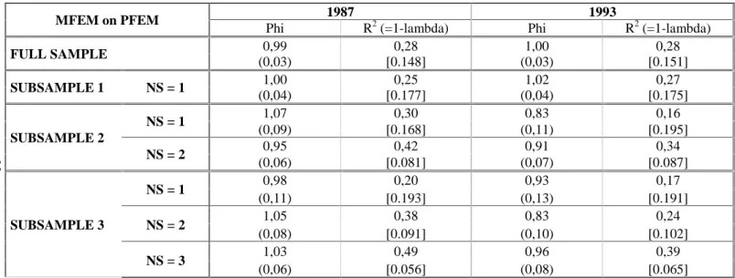
In this illustrative application where we have both the sampling error-ridden employee-based variable and the true firm level variable (or at least a rather good measure of it), we can in fact directly regress the former on the latter. We thus can check whether in such regressions the slope coefficients ϕ are indeed about equal to one as expected. If this is the case, the regression correlation coefficients R2 will give us new estimates of the ratios (1- λ) of the true variances to the measured ones, or equivalently the regression mean square errors (MSE) will give us new estimates of the sampling error
Table 4: Regressions of estimated female proportion on true female proportion:
slope coefficient Phi and R2 (=true variance ration (1-lambda) if Phi=1)
1987 1993
MFEM on PFEM
Phi R2 (=1-lambda) Phi R2 (=1-lambda) 0,99 0,28 1,00 0,28 FULL SAMPLE (0,03) [0.148] (0,03) [0.151] 1,00 0,25 1,02 0,27 SUBSAMPLE 1 NS = 1 (0,04) [0.177] (0,04) [0.175] 1,07 0,30 0,83 0,16 NS = 1 (0,09) [0.168] (0,11) [0.195] 0,95 0,42 0,91 0,34 SUBSAMPLE 2 NS = 2 (0,06) [0.081] (0,07) [0.087] 0,98 0,20 0,93 0,17 NS = 1 (0,11) [0.193] (0,13) [0.191] 1,05 0,38 0,83 0,24 NS = 2 (0,08) [0.091] (0,10) [0.102] 1,03 0,49 0,96 0,39 SUBSAMPLE 3 NS = 3 (0,06) [0.056] (0,08) [0.065]
MFEM: estimated female proportion; PFEM: "true" female proportion.
The regressions do not include industry and size dummies and do not control for skill composition; they differ only slightly from the regressions with industry and size dummies and skill composition variables
Standard errors are shown in ( ) and mean square errors (MSE) in [ ]. For other footnotes see Table 1.
24
variances. 24 We can then verify whether these estimates of (1- λ) and of the error variances are about equal to the ones independently computed on the basis of the (across employee) within firm variance of the employee based variable.
Our estimates of the slope and correlation coefficients ϕ and R2 in the regressions of MFEM on PFEM are shown in Table 4 for the full sample and the different sub-samples. What we see is clearly what we expected. The estimated slope coefficients are not significantly different from one. The R2 agree roughly, on the whole, with the corresponding estimates of (1- λ) in Table 2. They tend, however, to be higher, which again points in the direction of a modicum of random errors in PFEM: respectively 0.42 as against 0.31, and 0.34 as against 0.25 for the sub-samples with two interviewed employees in 1987 and 1993; and similarly 0.49 as against 0.39, and 0.39 as against 0.39 in the sub-samples with three surveyed employees.25
4. Conclusion
We hope to have convincingly shown in this paper that information collected from employees can be a great help in overcoming some of the major data difficulties increasingly encountered in firm econometric analyses, whether simply due to the unavailability of an easy measured variable or more deeply related to intrinsic problems in defining the relevant variables. We have also tried to convey the optimistic idea that this can be done by only surveying a few randomly chosen employees per firm, and would be very worthwhile even at the limit when one has only sub-samples with two or three surveyed employees, as in our illustrative application. We have also explained that the method to be followed, in the usual case of a linear regression model, is easy enough to implement, consisting of an application of the classical errors in
24 Note that if the OLS estimated ϕ are about equal to one, the estimated slope coefficients in the
reverse regressions of the true variable on the observed one are the regression R2 (and therefore less than one).
25
Note that, although they reflect the same evidence, the corresponding differences in terms of the regression MSE and of the estimated error variances seem more pronounced; they are the following: 0.08 as against 0.04, and 0.09 as against 0.03 for the sub-samples with two interviewed employees in 1987 and 1993; and similarly 0.06 as against 0.04 in the sub-samples with three surveyed employees in both 1987 and 1993.
25
variables framework, when one can obtain an independent estimate of the error variance-covariance matrices.26
Our framework and method, as we have presented and illustrated them here, can be in fact extended or generalized in various other contexts. We have considered them in particular in the case of a cross-sectional analysis of firms, but they can be similarly applied to a panel data analysis. In a panel data application we will not need that the surveyed employees be the same (or even be the same number) for the same firm in the different years of the panel (as long as being randomly chosen each year). The real problem will be in fact the basic one of the magnification of random errors of measurement in variables, and in the present instance the sampling errors in the employee-based variables, when one typically turns to within firm or differencing transformations in an attempt to control for unobserved correlated firm effects.27
We have also considered that the employee based variable (xi) is a mean
variable and estimated as such (as the firm average of the individual xih for the
surveyed employees in the firm), but in principle this variable could also be for example a variance or any given quantile and estimated accordingly (by the firm variance and quantiles of the xih). Here also the problem will be the
magnitude of the sampling error variance (involving for example in the case of a variance the within firm fourth moment of xih).
Our framework can be extended as well in contexts where the units of observation can be different from that of the employee and the firm as considered here. Indeed it has been already used in such contexts. One which is now well known in practice is that of so called pseudo-panel, where the units are "cohorts" defined by some common characteristics (like age, sex and occupation). In this case all the aggregate variables measured for the observed
26 Besides the application of our framework in this paper and previously in Greenan and
Mairesse, 1996, the only application which is to our knowledge quite comparable is that by Cockburn and Griliches, 1988. In their firm level investigation of the stock market’s valuation of R&D and patenting activities, the two authors try to take advantage of error-ridden indicators of appropriability at a detailed industry level (not the firm level), which are based on the answers of the surveyed firms by industry (not the surveyed employees by firm) in the "Yale survey on industrial R&D". They find, however, contrary to us, that in many cases their estimates of the true variance of these indicators are about zero (with estimated error variance being as large as the observed variance conditional on the other variables in the analysis), implying that these indicators do not bring new information beyond that already captured by the other variables.
27
For a recent exposition of the problem in the context of the estimation of a production function, see Griliches and Mairesse, 1998.
26
cohorts are error-ridden estimates of the true values for the full cohorts; and an errors in variables approach like the one considered here can be implemented to correct for the problem when of importance (i.e., when the number observations within cohort is small).28
In fact both our approach and the pseudo-panel approach for correcting errors in variables biases go back to a much earlier literature on either using repeated observations on the error-ridden variables in the equation of interest, or in grouping observations and estimating the equation on the group means.29 These two methods are technically equivalent, but they differ in terms of the requirement they put on the data, and in terms of exact interpretation of the estimated equation. Both can be applied the context of a cross-section, a single time-series or a panel.30 The originality of our approach like that of pseudo-panels is not really in the technique but in its potential domains of application. In recent years the development of pseudo-panels has been fruitful in providing new sources of data and in extending the possibilities of investigation in consumer or labor economics in particular; we hope that our approach will have a similar success in allowing for the construction and use of more comprehensive data sets in econometric studies of the firm.
28
See Deaton, 1985, for an original exposition of the method, and Verbeek, 1996, for a survey. For an interesting related application to an analysis of wage differentials in which in particular the authors extend the method to wage quantiles estimated on cells by age, education, sex and race, see Card and Lemieux, 1996.
29
See Tukey, 1951, and Madansky, 1959, for using repeated observations in an errors in variables model and Malinvaud (chapter 10), 1970, for grouping observations.
30 One of the advantage of a panel with repeated observations for the error-ridden variables, as
we just suggested above, or a pseudo-panel with group observations is of course in allowing to directly control for unobserved correlated fixed effects and therefore in helping to correct for both errors in variables and omitted variables biases.
27
References
CARD, David and LEMIEUX, Thomas "Wage Dispersion, Returns to Skill, and Black-White Wage Differentials", Journal of Econometrics, 74, (1996): 319-361.
DEATON, Angus "Panel Data from Time-Series of Cross-Sections", Journal of Econometrics, 30, (1985): 109-126.
COCKBURN, Ian and GRILICHES Zvi "Industry Effects and Appropriability Measures in the Stock Market’s Valuation of R&D and Patents, The American Economic Review, 78(2), 1988: 419-423. For more details, see Appendix A, "Sampling Errors in the Appropriability Measures", in NBER Working Paper 2465 (December 1987).
FULLER, Wayne A. "Measurement Error Models", John Wiley & Sons, New York, 1987.
GREENAN, Nathalie and MAIRESSE, Jacques (1996) "Computers and Productivity in France: Some Evidence", NBER Working Paper 5836. Forthcoming in Information Technology and the Productivity Paradox, edited by Paul A. David and Edward W. Steinmuller, London, Harwood Academic Publishers, (1999): 141-167.
GRILICHES, Zvi and RINGSTAD, Vidar "Errors in the Variables Bias in Nonlinear Contexts", Econometrica, 38, (1970): 368-370.
GRILICHES, Zvi and MAIRESSE, Jacques "Production Functions: The Search for Identification", in Econometrics and Economic Theory in the 20th Century: The Ragnar Frish Centennial Symposium, edited by Steinar Ström, Cambridge University Press, 1998.
HAEGELAND, Torbjorn and KLETTE, Tor Jacob "Do Higher Wages Reflect Higher Productivity? Education, Gender and Experience Premiums in a Matched Plant-Worker Data", in The Creation and Analysis of Employer-Employee Matched Data, edited by John D. Haltiwanger, Julia Lane, James Spletzer, Jules Theeuwes and Kenneth C. Troske, Amsterdam, North Holland, 1999.
MADANSKY A. "The Fitting of Straight Lines When Both Variables Are Subject to Error ", Journal of the American Statistical Association, (1959): 173-205.
28
MALINVAUD Edmond, Statistical Methods of Econometrics, 2d ed., Amsterdam, North-Holland, 1970.
TUKEY J. W. "Components in Regression", Biometrics, (1951): 33-70. VERBEEK Marno "Pseudo Panel Data" in The Econometrics of Panel Data,
edited by Matyas Laszlo and Sevestre Patrick, Boston, Kluwer Academic Publishers,1996.