Modeling protein evolution using secondary structures

(1)

Modeling protein evolution using secondary

structures

By

Zia Mohaddes

Bioinformatics Program

Faculty of Graduate Studies

Thesis submitted to the Faculty of Graduate Studies for obtaining the degree of MSc in Bioinformatics

August, 2010

© Zia Mohaddes, 2010

Université de Montréal Faculty of Graduate Studies

(2)

Faculty of Graduate Studies

This thesis is entitled:

Modeling protein evolution using secondary structures

Presented by: Zia Mohaddes

Evaluated by a jury composed of the following people:

Dr. Nadia El-Mabrouk, Chairperson Dr. Sylvie Hamel, Research Supervisor Dr. Andreea-Ruxandra Schmitzer, Co-Director

(3)

Abstract

Protein evolution is an important field of research in bioinformatics and catalyzes the requirement of finding alignment tools that can be used to reliably and accurately model the evolution of a protein family. TM-Align (Zhang and Skolnick, 2005) is considered to be the ideal tool for such a task, in terms of both speed and accuracy. Therefore in this study, TM-Align has been used as a point of reference to facilitate the detection of other alignment tools that are able to accurately model protein evolution. In parallel, we expand the existing protein secondary structure explorer tool, Helix Explorer (Marrakchi, 2006), so that it can also be used as a tool to model protein evolution.

Keywords: Protein evolution, tools, comparison of tools, sequence based alignments, and structure based alignments.

(4)

Résumé

L’évolution des protéines est un domaine important de la recherche en bioinformatique et catalyse l'intérêt de trouver des outils d'alignement qui peuvent être utilisés de manière fiable et modéliser avec précision l'évolution d'une famille de protéines. TM-Align (Zhang and Skolnick, 2005) est considéré comme l'outil idéal pour une telle tâche, en termes de rapidité et de précision. Par conséquent, dans cette étude, TM-Align a été utilisé comme point de référence pour faciliter la détection des autres outils d'alignement qui sont en mesure de préciser l'évolution des protéines. En parallèle, nous avons élargi l'actuel outil d'exploration de structures secondaires de protéines, Helix Explorer (Marrakchi, 2006), afin qu'il puisse également être utilisé comme un outil pour la modélisation de l'évolution des protéines.

Mots-clés : L’évolution des protéines, des outils, comparaison des outils, des alignements de séquences, des alignements de la structure.

(5)

List of Tables

Table 2.1. Structural alignment tools...…….….…..27

Table 3.1. Three types of correlation between protein families...69

Table 3.2. Protein families used by HE database...69

(8)

viii

List of Figures

Figure 1.1. Amino acid structure ……..………...…….….…..5

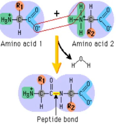
Figure 1.2. Formation of peptide bonds ………...…….….…..6

Figure 1.3. Amino acids ……….……...…….….…..6

Figure 1.4. Different levels of protein structures……...…….….…..8

Figure 1.5. Polypeptide chain torsion angles...…….….…..9

Figure 1.6. The alpha helix...…….….…..9

Figure 1.7. An example of a pleated beta sheet...…….….…..10

Figure 1.8. Anti-parallel and parallel beta sheets...…….……11

Figure1.9. Phylogenetic trees of chemokines and chemokine receptors...13

Figure 1.10. Protein-protein interactions and the evolutionary rate...15

Figure 1.11. Multiple sequence alignment...17

Figure 1.12. Pairwise structural comparison...19

Figure 1.13. RMSD...20

Figure 1.14. Abl tyrosine kinase and human p38 serine kinase...21

Figure 1.15. Structural patterns of two globins molecules...23

Figure 1.16. Correlation coefficient for protein families...24

Figure 2.1. Structural representation of DALI...27

Figure 2.2. Schematic view of DALI algorithm...28

Figure 2.3. Secondary structure elements as vectors...29

Figure 2.4. Alignment of secondary structure vectors...30

Figure 2.5. A similarity matrix using AFP...32

Figure 2.6. Superposition of two protein structures...34

Figure 2.7. STRAP...35

Figure 2.8. Low order value optimization problem...36

Figure 3.1. Common phylogenetic tree terminology...38

Figure 3.2. Construction of a phylogenetic tree...40

Figure 3.3. Correlation coefficients for the Small Kunitz……...47

Figure 3.4. Correlation coefficient for the Serpins family...47

(9)

ix

Figure 3.6. Correlation coefficient for the calmoduline-like family...49

Figure 3.7. Correlation coefficient for the Fe-mn-Superoxide-dismutase family...50

Figure 3.8. Correlation coefficient for the TIM family...50

Figure 3.9. Comparison between the structure-based and sequence-based phylogenetic

trees...52

Figure 4.1. The secondary structure search view within Helix Explorer. ...55

Figure 4.2. The Helix Explorer neighbour view...56

Figure 4.3. Distance measures used in the Helix explorer ...57

Figure 4.4. Angle betweenhelices………...57

Figure 4.5. Secondary structure properties ...58

Figure 4.6. Architecture of helix explorer...59

Figure 4.7. Detection of correspondence between the helices...62

Figure 4.8. The comparison between the HE and structure-based phylogenetic

trees...63

(10)

x

Acknowledgement

First and foremost I would like to thank my supervisor, Sylvie Hamel, for been extremely supportive, understanding and approachable throughout my study and for giving me the privilege to be her student. I would love to also thank my co-director, Andreea Schmitzer for her ongoing support and encouragement.

I would like thank the responsible of the Bioinformatics courses, Marie Pageau, Gertraud Burger, Hervé Philippe and Nicolas Lartillot for giving me the opportunity to take part in their courses. I would like to also thank everyone in lbit lab for creating a very comfortable and friendly ambiance.

At last, not least, I would like to thank my mother for believing in me and for giving me all the supports I needed throughout my study. Also I would like to thank my best friend, Eli, who provided me the motivation and support that I needed to move to Montreal and to continue my master.

(11)

xi

Abbreviations

DNA Deoxyribonucleic Acid

RNA Ribonucleic Acid

HTML HyperText Markup Language

mmCIF MacroMolecular Crystallographic Information File

NCBI National Center for Biotechnology Information

OpenMMS Open MacroMolecular Structures

PDB Protein Data Bank

PDBj Protein Data Bank Japan

PDBML Protein Data Bank Markup Language

(12)

2

Introduction

Protein comparison has been used extensively in bioinformatics on topics ranging from protein structure modeling to protein evolution. Several alignment tools, including but not limited to, DALI (Holm and Sanderand, 1993), CE (Shindyalov and Bourne, 1998b), Lovoalign

(Martínez et al., 2007b), LOCK2 (Singh and Brutlag, 1997), and TM-Align (Zhang and Skolnick, 2005) have been developed, all of which incorporate different structural alignment algorithms. These alignment tools aim to compare structures quickly and accurately, in order to facilitate modeling of the protein structure and overcome other bioinformatics obstacles. There are several steps involved in the comparison of protein (Eidhammer et al., 2004). First, a specific

characteristic (or feature) such as the distance between secondary structures is identified upon which the comparisons will be made. Next, an appropriate algorithm is selected, and used to detect the optimal alignment. Finally, the alignment is validated using different criteria to

measure the accuracy and quality of the given alignment as discussed further in the article written by Hitomi Hasegawa and Liisa Holm (Hasegawa and Holm, 2009).

A number of methods for comparing protein alignment tools have been developed and tested, the result of which is that TM-Align is considered to be faster and more accurate than other alignment tools due primarily to its optimal TM-score function. TM-Align performs a pairwise structural alignment using a dynamic programming algorithm and TM-score rotation matrix (Zhang and Skolnick, 2005; Teichert et al., 2007; Madhusudhan et al., 2009).

Protein evolution is an important field of study that addresses questions of how proteins evolve and change over a period of time. Protein evolution has diverse applications in

bioinformatics, such as, probing the method by which two binding proteins co-evolve through complementary changes in each other (Goh et al., 2000); improving homology modeling techniques, which involves modeling the 3D structure of a specific protein sequence (Pál et al., 2006) and helping us understand the relationship between the evolutionary distance and number of protein-protein interactions of a protein (Fraser et al., 2003; Martínez et al., 2007a). The importance of using 3D information in modeling the evolution of proteins has been emphasized in multiple articles due to the fact that structures of proteins are more conserved than protein

(13)

3 sequences (Lesk and Chotia, 1980; Chothia and Lesk, 1986; Holm and Sander, 1997; Bromham and Leys, 2005).

In fact, we agree that the choice of the alignment tool does affect the accuracy of the modeling of the evolution of a given protein family, and as a result this project intends to achieve three goals. Firstly, we are hoping to objectively determine the alignment tool most suited to the task of accurately modeling protein evolution when used in concert with TM-Align as a point of reference, due to its proven accuracy and speed. This will be accomplished by computing the distance between the phylogenetic trees resulting from each of the alignment tools chosen for comparison: CE, Lovoalign and LOCK2. Secondly, the performance of each of the alignment tools will be tested by applying them to protein families that have poor correlation between structure-based and sequence-based phylogenetic trees. This will be done by comparing the phylogenetic trees obtained from each of the four alignment tools (TM-Align, CE, Lovoalign and LOCK2) with the phylogenetic trees obtained by PhyML, which is a fast and accurate algorithm to estimate large phylogenetic trees (Guindon and Gascuel, 2003). The motivation for this idea comes from the PALI database study (Balaji et al., 2001). Finally we will aim to determine if the HE database can be used as a tool for modeling the evolution of proteins using secondary structures.

In Chapter 1, I will provide a brief introduction to proteins including their structure and composition. In Section 1.2, the different levels of structures of protein structures, such as alpha helices, beta sheets and turns, are discussed. The concept and importance of protein evolution, as well as the methods used to infer it, including structured-based and sequence-based methods, are discussed in Section 1.3.

The six different structural comparison tools chosen for comparison in this paper will be introduced in Chapter2. These are: DALI (2.1.1)1_{, LOCK (2.1.2), CE (2.1.3), TM-align (2.1.4),} STRAP (2.1.5) and Lovoalign (2.1.6), as well as the scoring function and algorithms used by each of these tools.

(14)

4 In Chapter 3, the techniques that can be used to compare the previously described

structural alignment tools will be presented and discussed. Section 3.1, will provide an

introduction to phylogenetic tree inference and comparison, while Section 3.2 will introduce the various protein databases that are used to extract the necessary data. In Section 3.3, I will describe the accepted techniques used to compare and validate the alignment tools and Section 3.4 will detail the phylogenetic-based method that I have implemented in order to compare the different structural alignment tools. Finally, in Section 3.5, I will present the results obtained from these comparisons, and provide relevant discussions and conclusions.

The Helix Explorer (HE), a web-based tool that has been designed to centralize

secondary-structure-based information aimed at facilitating Protein Data Bank (PDB) querying, will be introduced in Chapter 4. In Section 4.1, I will discuss the development and initial

functionalities of HE. Additional functionalities that have since been added to HE will be outlined in Section 4.2, and the algorithm developed that provided us with the ability to model protein evolution, will be presented and discussed. Finally, in Section 4.3 I will discuss the results, of the comparison between the phylogenetic trees obtained using HE and the ones obtained using the four alignment tools, and suggested future improvements.

Finally, Chapter 5 presents a summary conclusion and discussion of the entire thesis.

(15)

5

Chapter 1. Protein Structures and Evolution

In this chapter, an introduction to proteins is provided, along with a description of their composition. I will then describe the different levels of structures (primary, secondary, tertiary and quaternary) for a given protein in Section 1.2. In Section 1.3, the concept and importance of protein evolution will be discussed, as well as the methods used to infer the protein evolution (such as structured-based and sequence-based methods). The information in this chapter is strongly inspired by “Introduction to Protein Structure” (Branden and Tooze, 1998).

1.1 Introduction to Proteins

The word protein is derived from the Greek word “proteios”, which means 'primary of the first rank’. Proteins, polymers of amino acids, are created through a process termed ‘translation’. Twenty natural different amino acids are commonly found in different proteins. Among these amino acids, a similar structure is conserved: with the exception of proline, they all have a hydrogen atom (H), an amino group (NH2), and a carboxyl group (COOH), all of which are attached to a central atom (Cα), as shown in Figure 1.1. However, what makes these amino acids unique is the R-group, commonly referred to as the “side chain”, attached to the central Cα. Each of the twenty natural amino acids has a different R-group, which is specified by its genetic code.

Figure 1.1. Amino acid structure, consisting of hydrogen atom (H), an amino group (NH2), a carboxyl

group (COOH) and a central carbon atom (Cα) (Moniz, 2007).

(16)

6 As shown in Figure 1.2, individual amino acids are joined together via peptide bonds through a condensation reaction between the carboxylic group of one amino acid and the amino group of the second, a process that releases one water (H2O) molecule. As additional amino acids are linked together, this process repeats, elongating the chain. However, in each amino acid chain, two amino acids will remain intact: the amino group of the first amino acid and the carboxyl group of the last amino acid, highlighted in green and blue in Figure 1.2.

Figure 1.2.Formation of peptide bonds by condensation reaction between the carboxylic group and amino group (Pearson, 2009).

(17)

7 As mentioned previously, there are twenty different standard amino acids, shown in Figure 1.3, that are used to synthesize proteins and other biomolecules. These amino acids can be divided into three different classes, according to the biochemical nature of their side chain. These classes are as follows:

a) Amino acids with strictly non polar chains: includes Glycine (G), Alanine (A), Valine (V), Leucine (L), Isoleucine (I), Phenylalanine (F), Proline (P), and Methionine (M).

b) Amino acids with charged polar side chains: chains can be either positively or negatively charged. Includes Asparatic acid (D), Glutamic acid (E), Lysine (K), and Arginine (R).

c) Amino acids with uncharged polar side chains: includes Serin (S), Threonine (T), Asparagine (N), Glutamine (Q), Tyrosine (Y), Cysteine (C), Tryptophan (W) and Histidine (H).

With the exception of glycine, which has two hydrogen atoms attached to the central Cα, each of the remaining nineteen amino acids is a chiral molecule, since each has four chemically different groups attached to Cα. Glycine residues are usually considered to be the most flexible amino acid, and are able to integrate easily into both hydrophobic and hydrophilic environments, due specifically to their single hydrogen atom side chains.

1.2 Proteins and their Structures

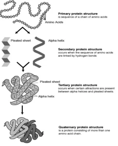
Any given protein has four levels of structure as shown in Figure 1.4. These are: the primary structure, which is a linear chain of amino acids; the secondary structure, which consists of highly regular structures defined locally; the tertiary structure, which is formed through attractions between secondary structures; and, finally, the quaternary structure, which is composed of more than one polypeptide chain. Due to the fact that some of the structural software used in this project incorporate secondary structure information, the different types of secondary structures will now be described in more detail.

(18)

8

Figure 1.4. The different levels of protein structures: primary, secondary, tertiary and quaternary (Huskey, accessed 2010)2_{(Huskey, 2010).}

There are three types of secondary structures found in proteins: the alpha helix (Section 1.2.1), the beta sheet (Section 1.2.2) and the turns (Section 1.2.3).

1.2.1 Alpha Helices

Alpha helices, important elements of secondary protein structures, were firstly described by Linus Pauling at the California Institute of Technology during the 1990s (Pauling, 1996).

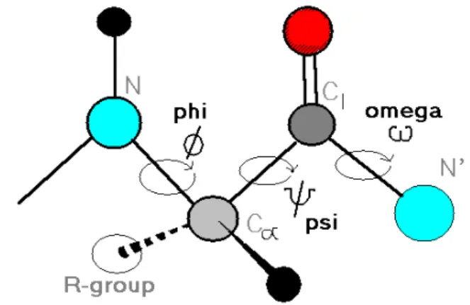
An alpha helix occurs when a chain of consecutive amino acids, formed through peptide bonds, all have their phi (φ) and psi angle (Ψ) in the range between -60o_{and -50}o_{, as shown in} Figure 1.5. In addition, both phi and psi angles can be visualized using the Ramachandran map

(19)

9 (Ramachandran and Sasisekharan, 1968). Since most of the residues in a helix are bonded in this manner, the helix is usually a rigid structure with very little internal space (Maccallum, 1997). Within an alpha helix, there are typically 3.6 residues per turn, and hydrogen bonding between the CO and NH groups of residues i and i+4 causes the formation of a right handed coil, as shown in Figure 1.6. Different variations of the alpha helix, such as the Pi helix and the 310 helix are created when i+5 or i+4 residues form hydrogen bonds with the residue i. The average length of an alpha helix, typically measured in globular proteins, averages ten residues and corresponds to three turns.

Figure 1.5. The three repeating torsion angles in the polypeptide chain are called phi (φ), psi (Ψ) and omega (ω). Black circles represent hydrogen atoms, grey circles represent carbon atoms, blue circles represent nitrogen atoms and red circles represent oxygen atoms (Wampler, 1996).

Figure 1.6. The alpha helix is one of the major elements of secondary structure in proteins. The O and N atoms are linked together by hydrogen bonds in the main chain (Hameroff, 1987).

(20)

10

1.2.2 Beta Sheets

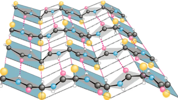
The beta sheet is another major structural element of globular proteins and is, in fact, a combination of several different regions of a polypeptide chain, called beta strands. Beta strands are typically made up of five to ten amino acids, all of which have their backbones in a fully extended conformation. In this formation, their side chains alternate directions, pointing upward, then downward, and so on. The beta strands must run parallel to each other so that a hydrogen bond can form between the N-H group in the backbone of one strand and the C=O group in the backbone of another strand. The beta sheet, more complex structures composed of these strands, are usually “pleated”, meaning that their Cα is slightly above or below the plane of the beta sheet, as shown in Figure 1.7.

Figure 1.7. An example of a pleated beta sheet where the oxygen (O) atoms are in purple, nitrogen (N) atoms in blue, hydrogen (H) atoms in white, Cα atoms in black, and side chains in orange (Preston, 2009).

Beta sheets can be structured in two very different ways, as parallel beta sheets or as anti-parallel beta sheets, as shown in Figure 1.8. In Parallel beta sheets, the amino acids of adjacent beta strands are coordinate in the same biochemical direction, meaning that the amino terminal and carboxyl terminal of each strand are adjacent. In anti-parallel configuration, individual beta strands alternate in direction, and the amino terminal of one strand is adjacent to the carboxyl terminal of the strand on either side.

(21)

11 The two different forms are distinguished by their specific patterns of hydrogen-bonding. Anti-parallel beta sheets have narrowly spaced hydrogen bond pairs alternating with widely spaced pairs while parallel beta sheets have evenly spaced hydrogen bonds (Keates, 1988).

Figure 1.8. Anti-parallel and parallel beta sheets, distinguished by different amino to carboxyl terminal

alignment and hydrogen-bonding pattern (Keates, 1988).

1.2.3 Turns

The two different secondary structure elements previously discussed, alpha helices and beta sheets, are usually connected in a globular protein by an irregularly shaped loop region called a turn. Loop regions, unlike other secondary structures, are usually found at the surface of the protein and as a result often form hydrogen bonds with nearby water molecules. Turns are typically rich in charged and polar hydrophilic residues, a feature that makes their presence easier to detect using prediction algorithms, unlike the other two secondary structures, which are usually embedded below the surface level of the protein, and lack the charged residues characteristic of turns.

(22)

12

1.3 Protein Evolution

1.3.1 Importance of studying protein evolution and protein structure

Protein evolution is a branch of biological study that focuses on the processes and mechanisms through which proteins change over time, while also addressing the question of why proteins evolve at different rates. Studying protein evolution also contributes to the reconstruction of past events that have given rise to the large variety of proteins in existence today (Doolittle, 1981).

Understanding the causes of observed variations in the evolutionary rate of proteins is essential for diverse and numerous fields, including molecular evolution, comparative genomics, and structural biology. The evolutionary rate of proteins can also be used to highlight the

importance of genetic drift and selection, as well as facilitate the identification of selective forces from genomic data. Analyzing protein evolution provides a unique method for understanding complex issues such as the evolution of speciation, due to rapid genetic evolution (Webster et al., 2003). Finally, it facilitates the discovery of functionally important sites used in protein design, peptides involved in genetic diseases, drug targets, and protein interaction partners.

The importance and benefits of studying protein evolution are well displayed through a number of studies, including protein-protein binding studies (Goh et al., 2000), homology modeling (Pál et al., 2006) , and the quantification of protein-protein interactions (Fraser et al., 2003).

1.3.1.1 Protein evolution in protein-interaction partners

Protein-protein binding plays an important role in both metabolic and signaling pathways. A pair of binding proteins must co-evolve, such that any divergent changes in one partner are complemented at the surface of the other, in order to maintain their mutual functioning. Unfortunately, using the results obtained from biochemical does not currently allow us to fully understand these interactions. Therefore, to gain a better understanding of the co-evolution of binding proteins, such as receptors and ligands, the available evolutionary information must be considered.

(23)

13

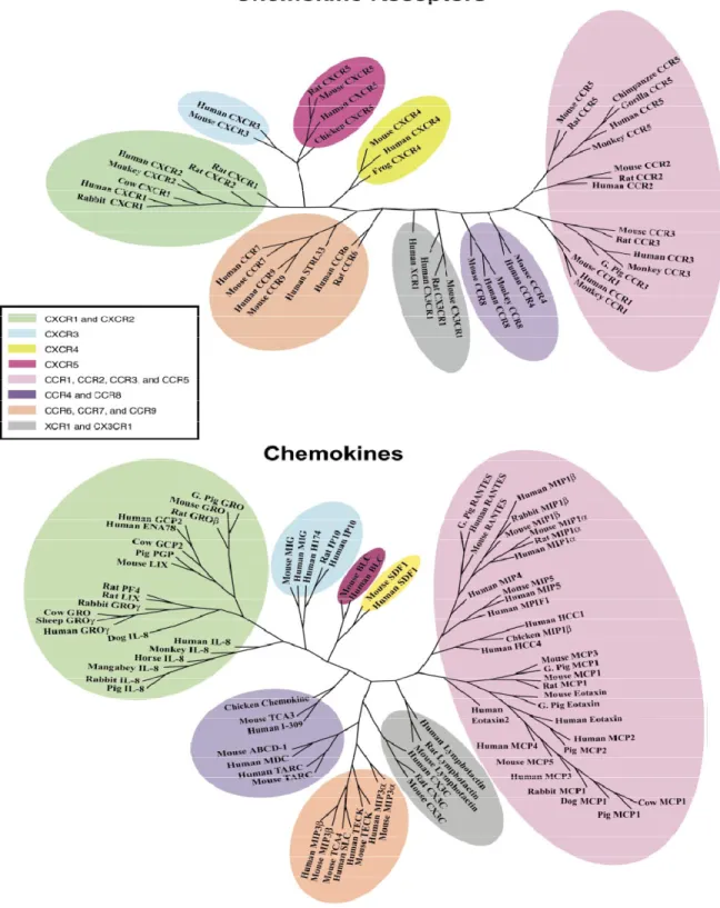
Figure 1.9. Phylogenetic trees of chemokines and chemokine receptors, where groupings among both families are shown by colored clusters. The diagrams are colored by their clustering patterns to show similar groupings among the chemokines and the receptors to which they bind (Goh et al., 2000).

(24)

14 Evolutionary information of proteins can be obtained using statistical comparisons

between the phylogenetic trees of protein families that interact with one another. For example, the phylogenetic trees of two chemokines families (a chemokine ligand and a chemokine G-protein coupled receptor) are shown in Figure 1.9. The colored clusters show the similar groupings between the two families. Using the two phylogenetic trees, corresponding to each of the chemokine proteins (receptor and ligand), one is able to calculate the correlation coefficient, which is a quantifiable measure of their co-evolution. Further mathematical analysis of chemokine protein co-evolution can be found in a study conducted by Goh et al. (Goh et al., 2000).

1.3.1.2 Protein evolution in homology modeling

An understanding of the mechanisms and pressures that caused a protein to evolve into a different protein will improve homology modeling, also known as comparative modeling, by identifying evolutionarily related proteins. Homology modeling techniques consist of modeling the 3D structure of a specific protein sequence by comparing its homologous protein, which is a protein sharing a common ancestor, with a known 3D structure (Pál et al., 2006). There are several steps required in homology modeling. First, a homologous (evolutionary related) protein must be identified. Next, the sequence of an unknown protein structure is aligned against the chosen, known, homologous structure. Once aligned, the information in the alignment will be used to construct and indentify the structurally conserved and variable regions represented by a series of coordinates. Finally, the determined structure is assessed and validated experimentally using free web-based software package called “what check”3_.

1.3.1.3 Correlation between the evolutionary rate of proteins and the number of protein-protein interactions

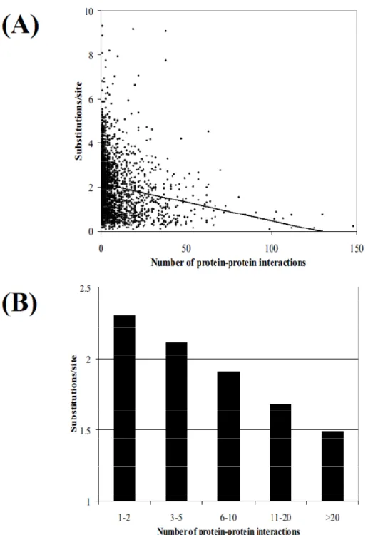
It has been shown through several studies that there is a highly significant negative correlation between the number of protein-protein interactions, in which a protein is involved, and the evolutionary divergence of this protein as shown in Figure 1.10 (Fraser et al., 2003). This correlation indicates that an increase in the number of protein–protein interactions will cause the rate of evolution of a protein to slow down due to structural constraints that must be maintained

3 _{‘What-check’ package contains a list of software used to validate the determined structures in}

(25)

15 to preserve all the interactions. It is important to note that this correlation can only be identified when using a large and complete set of protein-protein interaction data, as in the case of S.

Cerevisiae. Therefore this correlation cannot be generalized in other kingdoms of life, due to the

lack of complete set of protein-protein interaction data from other organisms.

Figure 1.10. The relationship between the number of protein-protein interactions and the evolutionary rate between S. Cerevisae and S. Pombe is shown. A) The relationship between the number of protein-protein

(26)

16

interactions and the evolutionary rate for all interaction data. B) The average evolutionary rates of genes categorized by their number of protein-protein interactions (Fraser et al., 2003; Martínez et al., 2007b).

In conclusion, there are many fields of study and situations that demonstrate the

importance of protein evolution. In all cases, either structural or sequential information is used in order to infer protein evolution. However, the question that remains is when to use either

sequence or structural information to compare distantly-related proteins in preference to the other, and why. One of the goals of this project is to answer this question by comparing the results obtained from selected structure-based and sequence-based protein comparison tools.

1.3.2 Comparison of sequence-based and structure-based inference of protein

evolution

This section will provide an overview of sequence-based and structure-based protein comparisons methods, as well as describe different studies in which the structure-based alignment is preferred.

1.3.2.1 Protein alignment using sequence information

Sequence alignment is a method used to identify regions of similarity that may be a consequence of functional, structural, or evolutionary relationships. In fact, the degree of similarity between amino acids at a given position indicates approximately how conserved this region is among different proteins. A pair of amino acids, one taken from each protein, is considered to be the smallest unit of comparison in sequence alignment.

Dynamic programming is widely used when performing sequence alignment. Every column in an alignment between two sequences represent an edit operation that can either be the replacement of an amino acid by another, the insertion or deletion of an amino acid or the

identity; for example the amino acid in a given position stay the same between the two sequences. Each edit operation has an associated cost, and the algorithm must detect the alignment that uses the edit operations with lowest cost (Needleman and Wunsch, 1970; Eddy, 2004).The alignment can then be read and considered as a way to transform one sequence into another. It should be noted that a distinction between the aim (which is finding the optimal solution), the cost, and the algorithm to maintain the cost should be always made.

(27)

17 Tools such as dotlet allow for pairwise sequence alignments (Junier and Pagni, 2000), while other tools, known as Multiple Sequence Alignment (MSA) tools, are able to produce alignment between multiple proteins. MSA tools are usually more computationally expensive and complex due to the greater alignment requirements. Results produced through MSA tools, such as those shown in Figure 1.11, provide information for each column of the alignment on the

mutations that occurred at one given site throughout the evolution of that protein.

Figure 1.11. Amino acid alignment of Connexin26 in different species (Dai et al., 2009)

Multiple sequence alignment tools incorporate different algorithms depending on the tool. ClustalW, the MSA tool used to produce the results shown in Figure 1.11, makes use of a

progressive alignment technique, which begins by aligning the two closest sequences to get an optimal alignment and then add the other sequences one by one in order to obtain the final multiple alignment (Thompson et al., 2002). Another MSA tool, muscle, uses iterative methods (Edgar, 2004), while hmmer uses a hidden markov model (Durbin et al., 2004). In this project, I will use ClustalW, an MSA tool using a progressive algorithm, (Thompson et al., 2002), and one of the most popular programs available for conducting MSA. Progressive algorithm consists of three steps: a) performing a pairwise alignment of all of the sequences; b) creating a phylogenetic tree using the obtained alignment scores; c) using phylogenetic relationships in the resulting tree to guide the sequential alignment of the sequences using a dynamic programming algorithm.

(28)

18 It is important to note that the quality of sequence alignments is unknown when there is a low sequence identity among the proteins. In such cases, the quality can be determined by comparing the obtained sequence alignment against an alternative protein alignment method, called structural alignment (Sauder et al., 2000), which is the subject of the rest of this chapter.

1.3.2.2 Proteins alignments using structural information

Since the discovery of the first proteins, the comparison of protein structures has been considered an extremely important task in structural and evolutionary biology. Establishing a correspondence between the residues of two protein structures is crucial in computational structural biology. Moreover, superimposition of similar protein structures and generation of structure-based sequence alignments will facilitate understanding of the evolutionary and thermodynamic constraints on a given fold, improve protein predictions, contribute to information about both individual proteins and protein structures, as well as help in the identification of homologous residues (Vesterstrom and Taylor, 2006; Hasegawa and Holm, 2009). Structural comparison is considered to be very efficient in providing information about common ancestry when dealing with homologous proteins, in identifying common sub-structures when dealing with non-homologous proteins, and in classifying proteins (Illergård et al., 2009).

The most natural way of comparing two objects, each represented by a collection of elements, is to determine the correspondences between them. This correspondence, or structural alignment, is usually based on the Euclidean distance of their central Cα atoms. Generally, the pairwise structural comparison of proteins can be divided into four major steps:

1) First, specific features are extracted, such as protein 3D coordinates, physiochemical properties of residues, sequential order of residues along the back bone, distance between two amino acids, and structural arrangement of secondary structures.

2) The extracted features are then used by comparison algorithms to detect a

correspondence or equivalence between two proteins based on certain constraints. These algorithms are explained further in Section 2.2 (Hasegawa and Holm, 2009).

(29)

19 system or threshold. There are different scoring schemes available, depending on

whether the structural representation is 3D, 2D (i.e. distance matrix or contact maps), or 1D (i.e. structural profile). A detailed list of these scoring schemes, according to their representation, can be found in a paper by Hasegawa and Holm (Hasegawa and Holm, 2009).

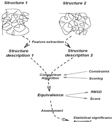
4) Finally, different evaluation tests are carried out to further measure the accuracy and quality of the alignments, as well as the ability of the alignment score to distinguish between homologous and unrelated proteins (Eidhammer et al., 1999; Eidhammer et al., 2004; Hasegawa and Holm, 2009). These properties will be discussed in more detail in Section 3.2. The schematic overview of these major steps is presented in Figure 1.12.

Figure 1.12. Pairwise structural comparison framework which includes: 1) feature extraction, 2) comparison algorithm 3) scoring schemes, and 4) assessment and validation (Eidhammer et al., 1999).

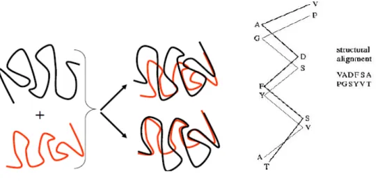
Despite the lack of a universally acknowledged definition of what constitutes structural similarity, there is a strong tradition of visualizing structural alignments by least square

(30)

20 procedure involves the superposition of the 3D structure of one protein onto the 3D structure of a second protein domain such that all the atoms fit together as closely as possible. The average spatial superposition detects a correspondence between the residues, based on the 3D structures of proteins, by identifying the highest number of atoms aligned with lowest Root Mean Square Deviation (RMSD) for the two given proteins, as shown in Figure 1.13. RMSD is the sum of the distances between residues in proteins A and B at position i divided by the total number of amino acid residues, as described by the following formula:

RMSD (A, B) = 2 1

/

1 N

N

d(a

,

b

_i

)

i= i

∑

However, RMSD has a number of pitfalls. First of all, identical RMSD in two different structural alignments (superposition) doesn’t necessarily suggest the same structural divergence, since they may not have the same number of “topologically equivalent Cα atoms”. Additionally, optimal alignment doesn’t always guarantee the minimal RMSD. And finally, significance of RMSD is size dependant.

To overcome these issues, some structural alignment algorithms, which will be explained in Section 2.1, have proposed different structural metrics that incorporate the size of the proteins, as well as the number of equivalent Cα atoms, into the RMSD measure. Structural distance metric (SDM), which is utilized by the structural alignment program STAMP (Russel and Barton, 1992), is an example of an algorithm featuring such improvements.

Figure 1.13. Given two protein structures, the goal is to find a transformation that superposes the two structures such that the RMSD is minimized. RMSD is the sum of the distances between residue a in the protein A at position i, and residue b in the protein B at position i divided by the number of residues (N).

(31)

21 The two protein alignment techniques, sequence-based and structure-based, have been described in Sections 1.3.2.1 and 1.3.2.2 respectively. The next section will describe which of these techniques can be applied when inferring protein evolution.

1.3.2.3 Inferring protein evolution using structural information

Evolution has produced homologous proteins whose sequences of amino acids have diverged significantly, but which have also maintained very similar structures. A popular example is the comparison of mouse abelson cytoplasmic tyrosine kinase to human p38 serine kinase as shown in Figure 1.14. Although they only have 28% sequence similarity, they have managed to maintain a common 3D structure.

Figure 1.14. Structural comparison between two kinase proteins: mouse Abl tyrosine kinase and human p38 serine kinase. Purple indicates alpha helices and yellow beta sheets in both proteins (Thorne, 2007).

Evolutionary changes usually occur in populations due to replacement, short deletions, and insertions of single amino acid residues. The extent of such changes, or perturbations, to a 3D structure will largely depend on the type and location of the evolutionary sequence changes. For example, some sequence mutations will cause the structure to alter, whereas others, which preserve the physicochemical properties of the protein, will have no impact on the structure. While it has been shown that most sequence mutations will be structurally conservative, the challenge is to map the evolutionary changes at the sequence level to the resultant protein structural perturbations (Illergård et al., 2009). This correspondence can help emphasize the advantage of structural comparison over the sequence comparison when dealing with divergent evolution, which has been discussed in various papers (Lesk and Chotia, 1980; Holm and Sander, 1997; Bromham and Leys, 2005).

(32)

22 There are a number of studies that demonstrate the importance of 3D comparison over the more traditional sequence comparison when dealing with distantly evolved proteins. In the following subsections, three of these studies (Lesk and Chotia, 1980; Holm and Sander, 1997; Balaji and Srinivasan, 2007), are explained, where the last sections is more emphasized since part of my project is based on it.

Analysis of conservation patterns in 3D and identification of new enzymes families

An interesting example is the identification of ten new enzyme families based on the similarity of the architecture of three known enzymes (urease, phosphotriesterase, and adenosine deaminase). The similarity of these three enzymes was detected based solely on a structural comparison that provided evidence of their distant evolutionary relationship. It is worth

mentioning that the importance of this similarity was previously unnoticed in traditional sequence comparisons(Holm and Sander, 1997). Additional details on how a structural comparison is conducted has been provided in Section 1.3.2.2.

Structural comparison of globins molecules

Similar research was conducted in which nine globin molecules were compared in order to answer the question of how different amino acid sequences maintain similar 3D structures. Figure 1.15 shows the comparison between two of these globins molecules, which have diverged widely in terms of their amino acid sequence, but have retained very similar secondary and tertiary structures. Both of these proteins have eight helices, which assemble in a common pattern. The variations in the geometrical arrangement of helices, which are produced by mutation and cause structural shift, in both globins molecules are interdependent in order to maintain similar function (Lesk and Chotia, 1980).

(33)

23

Figure 1.15. Structural patterns of two globins molecules are shown: a) the human deoxyhemoglobin; b) chiromus erythrocruorin molecules. The cylinders represent the helices in the globins molecules(Lesk and Chotia, 1980).

Correlation between sequence-based phylogenetic trees and structured-based phylogenetic tree

The final study relevant to this section, which the idea of comparing structure-based phylogentic trees was inspired from, presents an assessment conducted using 3D structure to model the evolution of homologous proteins (Balaji and Srinivasan, 2007). Using a dataset of 108 protein domain families of known structures, as well a series of constructed phylogenetic trees, a comparison of structural and sequence dissimilarities among pairs of proteins was made.

To conduct this comparison, a protein structural database called Protein ALIgnment Database (PALI), which contained structure-based and sequence-based distance matrices, as well as structure-based and sequence-based phylogenetic trees, was utilized. In order to align two proteins, a structural alignment tool called STructural AlignMent Program (STAMP) (Russel and Barton, 1992) was used. The result of this alignment was used to compute the Structural Distance Metric (SDM), which measures the extent of structural divergence, as well as the SEquence Distance Metric (SEDM) which quantifies the dissimilarity at the level of each amino acid sequence. These distances are placed into two different matrices: a structure-based and

(34)

sequence-24 based distance matrix, respectively. A clustering algorithm, such as the Neighbour Joining

Algorithm (NJ; explained further in Chapter 3) uses these matrices to generate the corresponding phylogenetic trees. Finally, as a measure of similarity between sequence-based and structure-based phylogenetic trees, a correlation coefficient is considered, where 1 indicates a perfect correspondence and 0 indicates no correlation.

Figure 1.16. Histogram depicting the distribution of the number of occurrences for every 0.1 interval of correlation coefficient for all 108 protein families considered in the analysis (Balaji and Srinivasan, 2007).

Comparison between the phylogenetic trees results in three different types of correlation coefficient distributions, which are based on the SEDM and SDM of all 108 families, as shown in Figure 1.16: a) families with good correlation (correlation coefficient > 0.6) between sequence

High Correlation

Intermediate Correlation Poor Correlation

(35)

25 based and structure-based phylogenetic trees; b) families with intermediate correlation

(correlation coefficient greater than or equal to 0.2 but less than 0.6); c) families with poor correlation (correlation coefficient < 0.2).

It was found that the correlation between the structure-based dissimilarity measures and the sequence-based dissimilarity measures was intermediate to high if sequence similarity among the homologous proteins was approximately 30% or greater. For protein families with low sequence similarity among the protein members, the correlation coefficient between the

sequence-based and structure-based dissimilarities was poor. This was due to domain movements for the multi-domain proteins and high flexibility in the case of small proteins.

Based on the three experiments outlined above, it can be concluded that protein evolution is best modeled using 3D structure when there is a low sequence similarity amongst the

homologous proteins.

Since protein structures are more conserved than sequences, it is logical to state that protein structures should be used to model the evolution of divergently related proteins. Structural comparison can be considered as a powerful “telescope”, enabling us to look back on earlier evolutionary history, as well as a more sensitive method than sequence comparison in determining protein function (Kolodny and Linial, 2004).

(36)

26

Chapter 2. Protein Structural Alignment

In the previous chapter, I have described the secondary structures present in proteins, the evolution of proteins, sequence-based and structure-based alignment techniques, and how protein evolution can be inferred through sequence and structural comparison. In this chapter, I will introduce six different structural comparison tools DALI, LOCK, CE, TM-align, STRAP, and Lovoalign as well as the algorithm and scoring system used by each of them.

2.1 Structural alignment tools

First, it is important to note that there is currently no universally accepted optimal way to align two structures. Choosing the right alignment tool or method depends largely on the question being asked. For example, is the goal to discover evolutionary relationships or structural

relationships? Do we need to compare a single structure against the entire database, or two structures to each other? Do we need to compare the whole structure (global similarity) or only some parts (domains) of the proteins (local similarity)? The different programs considered in this chapter each possess unique strength and weaknesses, depending on the type of questions being asked (Sierk and Kleywegt, 2004).

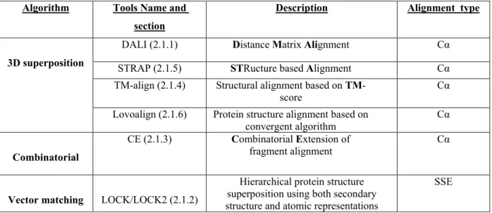
Table 2.1. A summary of the most used tools with a brief description and the type of alignment.

Algorithm Tools Name and section

Description Alignment type

3D superposition

DALI (2.1.1) Distance Matrix Alignment Cα STRAP (2.1.5) STRucture based Alignment Cα TM-align (2.1.4) Structural alignment based on

TM-score

Cα Lovoalign (2.1.6) Protein structure alignment based on

convergent algorithm Cα

Combinatorial

CE (2.1.3) Combinatorial Extension of

fragment alignment Cα

Vector matching LOCK/LOCK2 (2.1.2)

Hierarchical protein structure superposition using both secondary structure and atomic representations

(37)

27 Different structural alignment tools utilize different algorithms to measure the structural similarity between two proteins (Eidhammer et al., 1999). For example, STAMP (Russel and Barton, 1992), STRAP (Gille and Frommel, 2001) and DALI (Ropodi, 2003) use the least square superposition algorithm which requires an educated guess concerning the rigid-body

transformation. LOCK2, on the other hand, uses graph or vector matching algorithms (Shapiro and Brutlag, 2004). As evident by its name, CE makes use of the combinatorial extension (CE) algorithm (Shindyalov and Bourne, 1998a), while a dynamic programming alignment algorithm is used by TM-align (Zhang and Skolnick, 2005) and LOCK2 (Shapiro and Brutlag, 2004). Finally, Lovoalign uses a low order value optimization algorithm (Martínez et al., 2007b). The types of algorithms used are not limited to the above examples; rather, these examples are meant to portray the diversity of applied algorithms within structural alignment tools.

The name of each of these structural alignment tools along with their corresponding algorithm and the alignment type (Secondary structure element (SSE) or 3D structure (Cα)) are summarized in Table 2.1. I will now describe each of these tools in more details in the following sections.

2.1.1 DALI Structural alignment

The DALI algorithm was developed to achieve optimal pairwise alignment of protein structures. It assigns a one-to-one equivalence between the residues, based on the idea that similar 3D structures have similar intra-molecular distances. Each protein is represented as a 2D matrix of intra-molecular distances between Cα atoms, as shown in Figure 2.1a and 2.1b.

a) Protein A b) Distance matrix for protein A

Figure 2.1. Structural representation of DALI a) A graphical representation of the intra-molecular

distances between the Cα atoms of protein A; b) Intra-molecular distance matrix for protein A (Can, 2007).

1 2 3 4

(38)

28 DALI algorithm can be explained by comparing two topologically different proteins (P1 and P2), each composed of a three stranded beta-sheet. Thus, we have strands a, b, c for P1, and strands and a’, b’, c’ for P2. The goal of this algorithm is to construct a distance matrix given the protein 3D structure and then detects the common patterns between the distance matrices as shown in Figure 2.2.

Firstly, the two sub-matrices, belonging to strand pairs (a-b) for P1 and strand pairs (a’-b’) for P2, are compared to match their common patterns, as shown in Figure 2.2, a and b. Next, the alignments obtained from comparing fragment pairs (a,b)-(a’,b’)and (b,c)-(b’,c’) will be merged into a larger alignment, called a ‘seed’, consisting of strands (a,b,c)-(a’,b’,c’), as shown in Figure 2.2c. Finally, a Monte Carlo algorithm, in combination with a branch-and-bound and/or neighbour walk algorithm, is utilized to optimize the similarity scores, obtained from the seed alignment by either accepting or rejecting basic moves (insertion or deletion), and to build up the full alignment (Holm and Sanderand, 1993).

Figure 2.2. Schematic view of DALI algorithm; Step1 involves the comparison of two sub-matrices by matching their common patterns (a) and b)). Step2 consists of merging the alignments, obtained from the sub-matrix comparison, into a larger alignment called a seed (c). Step3 involves optimization of the alignment scores, using a Monte-Carlo algorithm, by applying either deletion or insertion moves (d) (Holm and Sanderand, 1993).

d) Monte-Carlo optimization c) Merging the two alignments a) Comparing fragments

(a,b) vs (a’,b’)

b) Comparing fragments (b,c) vs ( b`, c`)

(39)

29

2.1.2 LOCK algorithm: Hierarchical protein structure superposition using both

secondary structure and atomic representation

The following section is largely inspired by an article written by Singh and Brutlag (Singh and Brutlag, 1997). The LOCK algorithm is based on a hierarchy of structural

representation, ranging from the secondary structure level to the atomic level. This algorithm deals first with secondary structures, such as helices and strands, and then proceeds to atomic coordinate comparison. Secondary structures are processed first because they provide most of the stability and functionality of a protein, and as a result are more conserved than atoms during the evolution of a protein. The LOCK algorithm can be divided into two parts. Firstly, the alpha helices and beta strands are represented as vectors, as shown in Figure 2.3. The distance between two given vectors is computed by averaging the distances between the corresponding start, middle, and end points of the vectors. The angle is computed by taking the inverse cosine of the dot product of the two vectors.

Figure 2.3. Representing secondary structure elements as vectors (Singh and Brutlag, 1997).

These comparisons are made possible through the use of a set of seven scoring functions (S1 – S7 in Figure 2.4). Five of these scoring functions are orientation independent and two of these scoring functions are orientation dependent, based on distances and angles between the vectors. In fact, orientation independent score is based on the comparison of internal angles and distances between helices or beta sheets of each of the two proteins (i.e. comparing the angle between vector i and k in protein A to the angle between vector p and r in protein B). Conversely, orientation dependant scoring is based on comparing the individual vector distances and angles of each protein with the other protein (i.e. comparing the orientation of vectors i in protein A to the vector p in protein B), as shown in Figure 2.4. A dynamic programming algorithm is then used to

(40)

30 detect the best local alignment of the two sets of vectors which consist of finding the longest set of optimally matched pairs.

Figure 2.4. Alignment of secondary structure vectors (for proteins A and B) based on seven scoring functions (Singh and Brutlag, 1997).

The second part of the algorithm uses atomic coordinates to improve the vector alignment previously obtained by minimizing the RMSD (as defined in Section 1.3.2.2) between pairs of closest atoms from the two proteins. Finally, the obtained alignments are processed further by combining both the number of well aligned atoms and the RMSD to obtain the optimal alignment, known as the core alignment.

The use of secondary structure information allows the detection of both global and local similarities, as well as rapid and efficient initial superposition of the two proteins. The

hierarchical method of detecting optimal alignments among secondary structures, and then among atomic level alignments, makes the overall algorithm more flexible and faster. A comparison between the alignment results obtained by LOCK and those obtained using DALI demonstrates that LOCK manages to detect structural similarities accurately and also that it is able to detect a few low structural similarities missed by DALI.

(41)

31 A new version of LOCK, called LOCK2, has been developed to detect distant structural similarity by placing increased emphasis on the alignment of secondary structure elements (Shapiro and Brutlag, 2004).

2.1.3 Combinatorial Extension (CE) algorithm

The following section is heavily inspired by an article written by Shindyalov and Bourne (Shindyalov and Bourne, 1998b).

Instead of using dynamic programming, which is used by LOCK, or Monte Carlo

optimization, which is used by DALI, CE uses combinatorial extension of an alignment path. The alignment path is constructed by aligning short fragments from two proteins. The generated Alignment Fragment Pairs (AFPs), eight amino acids in size, are based on the orientation of secondary structures, RMSD, residue distances, and local secondary structure distances. The AFPs are placed into a similarity matrix, and an alignment path is extended by computing the distances Dij between AFPi from protein A and AFPj from protein B for all i and j, as shown in Figure 2.5 (Mettu, 2008).

Based on the previous definitions, the optimal alignment between two protein structures A and B, of length nA and nB, respectively, is the longest continuous path, P, of AFPs in the similarity matrix.

A score is used to evaluate the statistical significance of the longest alignment path. Z-score is computed by estimating the probability of finding an alignment path of the same length, with the same number or a smaller number of gaps, when two random structures are compared.

Comparisons made between CE and DALI, have shown that structural similarities involving small proteins are usually detected solely by CE, making CE well suited to the task of detecting similarities in very short proteins. In addition, its speed and accuracy in finding an optimal structure alignment make CE an ideal choice for database scanning and detailed analysis.

(42)

32 Unfortunately, the major limitation of CE is its inability to find alignments that have different topology4_.

Figure 2.5. A similarity matrix showing the calculation of distance Dij for alignment, represented by two

AFPs (AFPi for protein A and B at position i and AFPj for protein A and B at position j). CE aligns

structures and their sequences based on internal distances within each protein, rather than on inter-protein distance (Shindyalov and Bourne, 1998b).

2.1.4 TM-Align: A protein structure alignment algorithm based on the TM-Score

The following section is heavily inspired by an article written by Zhang and Skolnick (Zhang and Skolnick, 2005).

TM-Align uses the idea of the STRUCTAL (Levitt and Gerstein, 1998) and SAL (Kihara and Skolnick, 2003) algorithms, to speed up the process of identifying best structural alignment.

(43)

33 Briefly, TM-Align uses three types of initial alignments, which are described in more detail in this section.

The first initial alignment is carried out using dynamic programming to align the secondary structures elements (SSE) of two proteins. A score of either 1 or 0 is given for an identical SSE, and a score of -1 is given as a penalty for a gap opening.

The second initial alignment is obtained by selecting the smaller of the two proteins and being compared and aligning it against different parts of the larger protein. In this way, the alignment with the best TM score (rather than RMSD) can be chosen. The TM score is defined as:

Where d0(LTarget) is the distance, Lali is considered to be the number of aligned residues, and di is the distance between the ith pair of the aligned residues. It should be noted that the TM score combines three important features: alignment quality, alignment coverage and alignment accuracy. A TM-score is also normalized such that the resulting score is not dependent on the protein’s size.

The final initial alignment is performed using a gap-opening penalty of -1 and two score matrices: the secondary structure matrix and the distance score matrix. Using the aligned residues from the three initial alignments, described above, a heuristic algorithm then incorporates an iterative procedure to rotate the protein structures according to a TM-rotation-matrix.

The advantage of using TM-score is that it places more weight on close matches than on distant matches, the result of which is that it is more sensitive to the global topology of the proteins than RMSD, as shown in the Figure 2.6. According to Figure 2.6, the structural superposition has the same topology, but the difference in the loop region creates a high difference in RMSD, while resulting TM-scores remain very similar.

(44)

34

Figure 2.6. The superposition of two protein structures (1c0fS vs. model and 1c0fs vs. 1kcqA) shown to have similar topology according the TM-score measure (TM-score =0.70 and 0.67). However a loop variation can produce a rather high difference in the RMSD (10.5 and 1.9) (Zhang and Skolnick, 2005).

According to the comparison, the TM-Align algorithm is approximately four times faster than CE, and approximately twenty times faster than the DALI algorithm and has higher accuracy and coverage than the other programs. Additional studies, besides only the one discussed here, have also verified and emphasized the speed and accuracy of TM-align (Teichert et al., 2007; Madhusudhan et al., 2009). Due to the accuracy and speed of TM-align, a further comparison of this tool against other structural alignment tools will be made in Chapter 3.

2.1.5 STRAP (structural alignment program) with user friendly viewer

The following section is inspired largely by an article presented by Gille and Frommel (Gille and Frommel, 2001). STructural Alignment Program (STRAP) is a comprehensive tool with a user friendly interface used for the generation and refinement of multiple alignments of protein sequences using 3D coordinates. The efficiency of STRAP can be largely attributed to its simple visualization of Cα atom spatial distances within the alignment, as depicted in Figure 2.7. It is important to note that STRAP can only be used to perform alignments using either TM-align or a CE alignment program, and that it doesn’t incorporate its own protein structural alignment tool.

(45)

35 There are a number of tools that perform multiple sequence alignment by incorporating 3D information.However, these tools are not built to handle a large number of sequences (more than 400 sequences), and the result is that the sequences do not fit in one screen and require awkward scrolling. STRAP was designed to address these issues and has the capacity to handle a high number of sequences, in addition to allowing the viewing of spatial distance in sequence alignments. STRAP is capable of detecting structural relationships between aligned sequences, handling high number of sequence alignments by stacking several proteins in one line, and viewing and editing alignments in several synchronized windows, all coordinated through a user-friendly protein viewer. In addition to its simple viewer, STRAP has reduced memory

consumption, stores alignment results, and is extremely fast in loading proteins.

Figure 2.7. Screen-shot of STRAP showing an alignment of the β1 subunit of the proteasome colored according to charge and secondary structure types (Gille and Frommel, 2001).

2.1.6 Lovoalign: Protein alignment as a LOVO problem

Information provided in this section is inspired in large part by a detailed article written by Andreani et al. And Martinez et al. (Andreani et al., 2003; Martínez et al., 2007b). The

(46)

36 Lovoalign tool transforms the protein alignment problem into a Low Order Value Optimization (LOVO) problem. The LOVO problem is a generalization of the classic minimax problem, which aims to maximize the scoring functions in protein alignment, and it can be defined as follows: Given a set of real functions f1(x)….fm(x), the goal is to find x such that the maximum of f1(x)….fm(x) is maximal.

Figure 2.8. Protein alignment as a low order value optimization problem (Martínez et al., 2007b).

The LOVO method can be easily applied to the task of structural alignment. As

mentioned previously, the goal of structural alignment is to find a correspondence by minimizing the RMSD between the Cα atoms through the application of transformation (translation and rotation) to one of the protein structures. Based on this definition, a function (i.e. scoring

function) of rotation and translation can be defined using the obtained correspondences, as shown in Figure 2.8. Therefore, the goal of Lovoalign is to maximize the scoring function of each individual correspondence, and the correspondence with the maximal score will be selected as the optimal alignment.

The Lovoalign can be either used on the website5_{or downloaded on a Linux-based} computer. Not only is Lovoalign fast, but it has also successfully maximized the STRUCTAL score (used by STRUCTAL alignment), as well as other distant-dependant scores. The detailed steps of the algorithm can be found in the article by Martinez et al. (Martínez et al., 2007b).

(47)

37

Chapter 3. Comparison of structural alignment tools

In the previous chapter, six different alignment tools, including their functionalities, were described. In this chapter, I will introduce the techniques that can be used to compare the

previously described structural alignment tools. In Section 3.1, I will start with the introduction to phylogenetic tree inference and comparison. In Section 3.2, I will introduce the different protein databases used to extract the necessary data. In Section 3.3, I will describe the different

techniques used to compare and validate the alignment tools. In Section 3.4, I will describe the phylogenetic based method that I have utilized to compare different structural alignment tools. Finally, in Section 3.5, I will present the results obtained, as well as the relevant discussion and conclusion.

3.1 Phylogenetic tree inference and comparison

3.1.1 Definition and purpose of phylogenetic trees

This section is strongly inspired by a book on bioinformatics written by Mount (Mount, 2004).

Phylogenetics is an area of research concerned with identifying the genetic relationships between various organisms by relying on information extracted from DNA, RNA, or protein sequences (Potter, 2008).

An evolutionary tree, also known as a phylogenetic tree, depicts the evolutionary relationships between organisms. As shown in the Figure 3.1, a group of organisms, genes, or species can be used to construct a phylogenetic tree. A phylogenetic tree is composed of several different components. The leaves of the tree represent the taxa (a group of organisms), while internal nodes (also termed ‘divergence points’) represent the hypothetical ancestor of the taxa rooted at this node. Branches (or lineages) of a phylogenetic tree connect the different nodes. Finally, the ancestral node, which can be visualized as the root, represents the ancestor of all taxa presented at the leaves of the tree. Usually, the number of sequence changes that occurred prior to the point of separation or speciation can be characterized by the length of each branch. In a

(48)

38 situation where two species have the same branch length from their respective leaf to the common ancestor, it is suggested that they have evolved at relatively the same rate.

Figure 3.1. a) A simplified tree illustrating common phylogenetic tree terminology. A phylogenetic tree usually consists of the root, branches, internal nodes and leaves. b) The corresponding unrooted tree.

A phylogenetic tree is usually binary, meaning that only two branches stem from each node. A binary tree can either be rooted or unrooted; an unrooted tree is one that makes no assumptions about the position of the root, as shown in Figure 3.1b.

3.1.2 Multiple sequence alignment used to generate phylogenetic trees

To construct a phylogenetic tree, the protein sequence must first be aligned using a multiple sequence alignment tool. Once these results are obtained, a phylogenetic analysis algorithm is utilized to infer the resulting phylogenetic tree.

In this project, a specific protocol is used to infer the phylogenetic trees. As explained in Section 1.3.2.1, ClustalW can be used to perform an MSA for a series of protein sequences, and this is what has been done in this project. Gblocks (Castresana, 2000) is then used to extract poorly aligned regions or divergent regions from the MSA obtained via ClustalW (Thompson et al., 2002), while minimizing the loss of informative sites. Finally, the factored MSA can be used

A B C D E Root TAXA Internal Nodes Branches D E B A C Unrooted tree a) b)

Modeling protein evolution using secondary structures