Chen: Statistics Canada, Family and Labour Studies Statistics, Ottawa, K1A 0T6; Phone: 1-613-951-3807
Wen-Hao.Chen@statcan.ca
Duclos: Département d’économique and CIRPÉE, Pavillon DeSève, Université Laval, Québec, Canada G1K 7P4; Phone: 1-418-656-7096; Fax: 1-418-656-7798
jyves@ecn.ulaval.ca
Cahier de recherche/Working Paper 08-36
Testing for Poverty Dominance : an Application to Canada
Wen-Hao Chen Jean-Yves Duclos
Abstract:
The paper proposes and applies statistical tests for poverty dominance that check for whether poverty comparisons can be made robustly over ranges of poverty lines and classes of poverty indices. This helps provide both normative and statistical confidence in establishing poverty rankings across distributions. The tests, which can take into account the complex sampling procedures that are typically used by statistical agencies to generate household-level surveys, are implemented using the Canadian Survey of Labour and Income Dynamics (SLID) for 1996, 1999 and 2002. Although the yearly cumulative distribution functions cross at the lower tails of the distributions, the more recent years tend to dominate earlier years for a relatively wide range of poverty lines. Failing to take into account SLID’s sampling variability (as is sometimes done) can inflate significantly one’s confidence in ranking poverty. Taking into account SLID’s complex sampling design (as has not been done before) can also decrease substantially the range of poverty lines over which a poverty ranking can be inferred.
Keywords: Stochastic dominance, empirical likelihood, Canada, income distribution
1 Introduction
Making comparisons of monetary poverty across time and space usually neces-sitates making a substantial number of important methodological choices. First, there is the choice of the nominal measure of living standards. Is it income or consumption? Is it cash income or comprehensive income (including for instance the value of the consumption of non-marketed goods and services such as leisure and public goods and services)? Is it monthly, yearly or lifetime income? Does it include the imputed value of the service from assets and durable goods, in the form of housing and car ownership for example?
Second, there is the choice of procedures to compare individual-level real liv-ing standards. These procedures are needed because individuals differ in several dimensions other than their levels of nominal income. This includes differences in household sizes and composition — traditionally taken care of by the application of equivalence scales — and temporal and spatial differences in the prices faced by individuals — usually corrected for by the use of time- and space-dependent price deflators. Third, there is the choice of the unit of poverty analysis — is it the individual, the family or the household? — as well as whether we can assume equality of welfare across the members of a same family or household.
To be sure, some consensus has emerged over the best practice for some of these choices. For instance, it is usually recognized that the measure of income should be as comprehensive as possible, and that it should also adjust as much as is feasible for differences in price levels across time and space using the value of constant commodity baskets that are representative of the consumption habits of the poor. It has also become standard normative practice to consider the individual as the fundamental unit of welfare analysis. But other issues are more difficult to resolve, at least in practice. This is the case for instance for the choice of equiv-alence scales, for which there exists a myriad of possible forms and values, and for how equally welfare is distributed within a household, since this necessitates disentangling difficult within-household allocation issues.
Comparing poverty
Once a measure of individual welfare is agreed upon, there remain at least three other important sources of methodological sensitivity for poverty measurement. The main objective of this paper is to address them.
The first source of methodological sensitivity comes from the choice of a poverty line, be it absolute (such as the official US poverty line) or relative (such
as one half of median income). Agreement on such a choice is difficult since there exist many alternatively sound normative and statistical procedures for the estimation of poverty lines. Forcing the estimation or the use of a single poverty line usually amounts to forcing a value judgement, and is therefore essentially arbitrary.
Another important source of arbitrariness comes from the choice of a poverty index. Such a poverty index is needed to aggregate the distribution of individual welfare into a single number. There exists, however, a large pool of such indices in the scientific literature, and most of them can be shown to be quite sensible on normative grounds. Again, forcing the choice of a single poverty index would amount to enforcing an essentially arbitrary value judgement.
These sources of arbitrariness might not be of practical concern if they did not matter empirically. But comparisons of poverty (across time, regions, socio-demographic groups, or policy regimes, for instance) are often empirically sensi-tive to the choice of poverty indices and poverty lines. We often find for instance that poverty is greater in one region than in another for some poverty lines, but that the opposite is true for some other lines. This can occur for example when a region exhibits larges pockets of moderate poverty, but smaller pockets of se-vere poverty, than another one. A policy that redistributes from the not-so-poor to the very poor may be deemed to reduce poverty for some “distribution-sensitive” poverty indices, but to increase it for indices that are less sensitive to the inci-dence of extreme poverty. Given again that there is rarely unanimity as to the right choice of poverty lines and poverty indices, it follows that such sensitivity can seriously undermine one’s confidence in comparing distributions or in making policy recommendations.
Poverty measurement is finally sensitive to the choice of sample used to es-timate poverty for a population of interest. This naturally suggests the applica-tion of statistical inference techniques. Although the need for these techniques is widely agreed, surprisingly little of the empirical poverty literature actually ap-plies them. The failure to do so can lead to statistically insignificant differences being presented as reliable evidence on poverty differences. The need for statis-tical inference is even greater in the context of the complex sampling procedures that are typically used by statistical agencies. These procedures indeed often lead to greater sampling variability than the simple random procedures that are usually assumed by empirical poverty analysts.
Poverty in Canada
The above discussion is all the more pertinent in Canada as there has been a long-standing debate in that country over the meaning of the term “poverty”. In fact, the term “official poverty line” never existed in Canada. Almost all Canadian poverty work has nevertheless revolved around the definition of Statistics Canada’s Low Income Cutoffs (LICOs), which was introduced in early 1970s. These cutoffs are based on a somewhat arbitrarily posited relationship between income and ne-cessities such as food, shelter and clothing. Over the years Canadian researchers have used other measures to supplement the LICOs, including the low income measures (LIM)— that emphasize relative poverty — and the recently developed market basket measure (MBM) that attempts to identify an income threshold ly-ing between the poles of subsistence and social inclusion.1 Nevertheless, none of
these other measures can be considered to be free from arbitrariness in defining poverty or low-income thresholds.
Furthermore, given the difficulty of measuring resources and of defining poverty thresholds, the issue of choosing an ethically acceptable poverty aggregation in-dex has been rarely discussed in Canada. The usual practice is to calculate the headcount ratio, often called the poverty rate, which measures the proportion of individuals below a poverty threshold. Only occasionally have other indices, such as the average poverty gap, been used in addition to the poverty rate.2
Finally, nearly all empirical poverty or low income research in Canada and elsewhere derives their statistics from survey data (in Canada, this is currently the Survey of Labour and Income Dynamics) that are drawn using a complex
and multi-stage sampling design.3 As mentioned above, complex sampling
pro-cedures often lead to greater sampling variability. Unfortunately, poverty research in Canada has been forced to overlook that issue since the key sampling design identification variables (such as stratum, primary sampling unit and secondary sampling unit) were simply not available in the datasets. This raises an important reliability issue for all of the statistical comparisons of poverty found in existing studies of poverty in Canada. Indeed, the same reliability issue certainly arises for
1See Giles (2004) and Human Resources and Social Development Canada (2006) for a detailed
discussion on LICOs, LIM and MBM measures.
2Some exceptions include Osberg (2002) and Chen (2008). They both use
distribution-sensitive indices in addition to the poverty rates and they demonstrate that poverty comparisons can differ markedly with the aggregation index chosen.
3Only a handful of poverty and low income research uses data from administrative tax records
— such as the Longitudinal Administrative Database (see, for example, Picot, Hou, and Coulombe (2007).
all other countries although it has not, to our knowledge, been investigated in any of them, at least in the context of dominance testing.
Objective of paper
To help alleviate these concerns, the paper proposes and applies a methodology that checks for whether poverty comparisons can be considered robust to the choice of poverty lines and poverty indices. This methodology is based on tests for poverty dominance of a distribution (say, A) against another (B, say). In doing this, the paper focuses on ordinal comparisons of “distributions” (“In which year or region is poverty greatest?”) as opposed to cardinal comparisons (“How much poverty is there in a particular distribution?”). An important feature of the paper is also to propose and apply statistical tests of poverty rankings and thus to make poverty comparisons robust to sampling variability. This serves to help provide statistical confidence (in addition to normative confidence) in ranking A and B.
The most obvious advantage of the paper’s methodology is that it can provide clear-cut and robust conclusions on whether poverty is larger in A or in B. This serves among other things to avoid fixation on one or only a few poverty lines, thus avoiding costly debates and investment on the identification and the estimation of poverty lines. Furthermore, such conclusions are robust over a set of poverty indices, thus removing the need to argue and agree on the selection of aggregating procedures. Because of this, robust poverty rankings are also less susceptible to distorsion and misuse by policymakers and policy analysts, and can thus generate greater public confidence.
Not all poverty comparisons made using the paper’s methodology will end up being robust over wide ranges of poverty lines and broad classes of indices. In the absence of such robustness, the paper’s methodology can nevertheless be used to provide the more limited sets of measurement assumptions over which the poverty ranking of A and B does happen to be conclusive. This can therefore help clarify and settle methodological disputes over poverty rankings. It can also serve to highlight the differences in the distributions that create ambiguity in their ranking. Again, this can provide greater transparency in poverty analysis than the use of selective poverty statistics by policymakers and policy analysts.
In some cases, however, the use of this paper’s methodology will lead to the conclusion that the poverty ranking of A and B is too sensitive, either to the choice of measurement assumptions (poverty lines, poverty indices) or to the presence of sampling variability (the statistical significance of differences in poverty being too low). The poverty orderings will then be deemed to be ambiguous. This type
of outcomes may be thought of as being “negative”. We believe this would be an incorrect assessment of the value of such results. Ambiguous results reveal that ranking poverty across A and B could perhaps still be made but only at an assignable cost in terms of normative and statistical confidence.
An important feature of this paper’s methodology is then to focus away from thinking about poverty levels towards thinking about poverty rankings. Poverty levels are intrinsically arbitrary: their value necessarily depends on the precise measurement choices that are made. Poverty levels are also subject to sampling variability: statistically speaking, we can only think in terms of ranges of poverty levels, not about their precise values. Inference on poverty rankings can be a lot more precise. Since poverty rankings essentially deal with the sign of poverty differences, and not with their precise numerical value, they can be made both normatively and statistically strong.
The rest of the paper runs as follows. Section 2.1 illustrates briefly how poverty comparisons can be sensitive to the choice of important measurement assumptions. Section 2.2 outlines how a focus on robust poverty rankings can alleviate concerns for such sensitivity, and describes techniques for checking for poverty dominance. Section 3 presents procedures for testing dominance using two alternative sets of test statistics. Section 4 illustrates the application of the paper’s methodology using Statistics Canada’s Survey of Labor and Income Dy-namics.
2 Poverty rankings
2.1 Sensitivity of poverty comparisons
2.1.1 Ordinal sensitivityWe start by illustrating why and how poverty comparisons can be sensitive to the choice of measurement assumptions. Let the FGT indices of poverty (see Foster, Greer, and Thorbecke 1984) be defined for parameter α ≥ 0 and poverty line z as
PA(z; α) = Z z 0 µ z − y z ¶α dAF (y) (1)
where FA(y) is the distribution function for distribution A.
Consider the hypothetical example of Table 1. The second, third and fourth lines in the table show the incomes of three individuals in two hypothetical dis-tributions, A and B. Thus, distribution A contains three incomes of 0.4, 1.1 and
2 respectively. The bottom 3 lines of the table show the value of the two most popular indices of poverty, the headcount P (z; 0) and the average poverty gap
P (z; 1) indices, at two alternative poverty lines, z = 0.5 and z = 1. The poverty
headcount gives the proportion of individuals in a population whose income falls underneath a poverty line. At a poverty line of 0.5, there is only one such person in poverty in distribution A, and the headcount is thus equal to 0.33 (shown on the fifth line of Table 1. The average poverty gap index is the sum of the distances (normalized by z) of the poor’s incomes from the poverty line, divided by the total number of people in the population. For instance, at a poverty line of 1, there are 2 people in poverty in B, and the sum of their distances from the poverty line is ((1-0.6)+(1-0.9))=0.5. Divided by 3, this gives 0.166 as the average poverty gap in B for a poverty line of 1 (shown on the last line of Table 1).
At a poverty line of 0.5, the headcount in A is clearly greater than in B, but this ranking is radically reversed if we consider instead the same headcount index but at a poverty line of 1. The ranking changes again if we use the same poverty line of 1 but now focus on the average poverty gap P (z; 1): PA(1; 1) = 0.2 < 0.166 = PB(1; 1). Clearly, the poverty ranking A and B can be quite sensitive to the precise choice of measurement assumptions.
2.1.2 Cardinal sensitivity
As seen above in the context of Table 1, differences in simple poverty indices can be deceptive when it comes to order distributions. They can also quantify deceptively distances between distributions even when the poverty rankings are held constant. To illustrate this, consider Table 2 with distributions A and B and a poverty line z = 1. The three FGT poverty indices P (1; α) agree that poverty has not increased in moving from A to B. But the quantitative change in poverty varies significantly with the value of α. With the poverty headcount, poverty remains the same, but the average poverty gap falls by 33% and the “squared-poverty-gap” index (P (z; α = 2)) falls by 56%.
2.2 Poverty dominance
2.2.1 Poverty rankingsA focus on robust poverty rankings can fortunately allay the above sensitivity problems. Robust poverty rankings simply order distributions; for this, estimates of cardinal differences in poverty indices are not needed. The method described
below draws from the literature on stochastic dominance. Its application to poverty comparisons is thus usually denoted as poverty dominance. Important references to that literature include Atkinson (1987), Foster and Shorrocks (1988a) and Fos-ter and Shorrocks (1988b).
Making robust ordinal comparisons of poverty involves using classes of poverty indices. It is useful to define these classes by referring to “orders of normative (or ethical) judgements”, an order being denoted as s = 1, 2, .... Whether an ordering of poverty is valid for all of the indices that are members of a class of order s is tested through poverty dominance tests, which happen to be convenient variants of well-known stochastic dominance tests also of order s. When two poverty domi-nance curves of a given order s do not intersect, all poverty indices that obey the ethical principles associated to this order s of dominance then order in the same manner the two distributions.
2.2.2 First-order dominance
We focus in this paper on first-order poverty dominance comparisons, although it is relatively straightforward also to consider high-order dominance comparisons4.
The poverty indices that are ranked by first-order poverty dominance have four properties. The first is that they should show (weakly) a fall in poverty when-ever someone’s income increases, when-everything else being the same. These poverty indices must therefore obey a property akin to that implied by the well-known
Pareto principle.
The second property deals with differences in population sizes. It forces poverty indices to be invariant to adding an exact replicate of a population to that same population, and derives from the population invariance principle.
The third property follows from an anonymity principle: everything else being the same, whether it is an individual named a rather than b that enjoys some given level of income should not affect the value of a distributive index. It also follows from this property that interchanging two income levels should not affect the value of the poverty indices.
The fourth property follows from the focus principle: for a fixed poverty line z, poverty indices are invariant to marginal changes in those incomes that are above the poverty line z.
The first-order class of poverty indices — denote it by Π1(z+) — then
re-groups all of the poverty indices P (z) that are anonymous, that are population
invariant, that show a (weak) poverty improvement following an increase in in-comes below a poverty line z, that are insensitive to increases in any income above
z, and whose poverty line z does not exceed z+.
We then have (for a proof, see for instance Foster and Shorrocks 1988a):
Theorem 1 First-order poverty dominance
PA(z) − PB(z) ≥ 0 for all P (z) ∈ Π1(z+)
if and only if FA(y) > FB(y) for all y ∈ [0, z+]. (2)
An example of an ordering provided by Theorem 1 is shown in Figure 1. Fig-ure 1 shows two poverty dominance curves, one for A and one for B. FA(y) is always larger than FB(y) at all y between 0 and z+. Hence, we can invoke Theo-rem 1 to declare poverty in A, PA(z), to be larger than poverty in B, PA(z), for all of the poverty indices P (z) in Π1(z+) and thus for any choice of poverty lines z
below z+. Note that this orders poverty across a large class of poverty indices,
in-cluding all of the FGT indices as well as virtually all of the indices that have been proposed and used in the literature. Thus, this is a powerful ordering of poverty. In fact, we could extend it up to all of the poverty indices in Π1(z++) since we
have that FA(y) − FB(y) ≥ 0 for all y between 0 and z++. Π1(z++) is also the largest set of poverty indices that all declare poverty to be larger in A than in B.
Figure 1 provides an attractive and simple-to-understand test of the ranking of poverty across distributions. We saw that since we are able to order the distribution functions FA(y) and FB(y) over the range [0, z++], we are also able to order poverty across A and B for all of the poverty indices and poverty lines consistent with Π1(z++).
Practically speaking, however, we may not be able to do this. One reason for this is that testing over the entire range of [0, z++] may be statistically too
de-manding, since it involves comparisons of poverty dominance curves over ranges where there may be too little information. A proof that it is generally impossible to test down to the lower bound of 0 is given in Davidson and Duclos (2006). The sampling distribution of a crossing point such as z++in Figure 1 is provided
in Davidson and Duclos (2000), also suggesting that statistical prudence would usually prevent us from inferring dominance up to a point that is too close to z++.
Hence, it may make more practical and statistical sense to focus on poverty dominance restricted to a domain Z = [z−, z+], say, that lies strictly inside the
wider range of [0, z++]. From a normative point of view, there are also arguments
that favor such a restriction — some of them are reviewed in Davidson and Duclos (2006). This leads to the definition of a class of restricted first-order indices,
namely, indices that use poverty lines restricted to the range Z = [z−, z+]. The
indices that are members of Π1(Z) are insensitive to changes in incomes when
these take place outside of Z: they thus behave somewhat like the headcount index outside Z, being invariant to marginal changes in income either below z− or above z+.
3 Testing for poverty dominance
We now turn to how the conditions in Theorem 1 can be tested statistically. 5
Consider again two cumulative distribution functions FA and FB. As mentioned above, distribution B is said to poverty-dominate distribution A at first order if, for all y ∈ Z, FA(y) > FB(y). Testing for such dominance using sample data, however, requires leaping over a number of hurdles.
• First, there is the possibility that population dominance curves may cross when the sample ones (denote these by ˆFA(y) and ˆFB(y)) do not.
• Second, the sample curves may be too close to allow a statistically signifi-cant ranking of the population curves.
• Third, there may be too little sample information from the tails of the dis-tributions to be able to distinguish dominance curves statistically over the entire domain Z.
• Fourth, testing for dominance involves testing differences in curves over a large (or infinite) number of points in Z.
• Fifth, the overall testing procedure should take into account the dependence of the large number of tests carried out jointly over Z.
• Sixth, we should take into account of the sampling design of the survey.
• Finally, dominance tests are always performed with finite samples, and this may give rise to concerns whenever the properties of the procedures that are used are known only asymptotically.
5A considerable empirical literature has sought to test for stochastic dominance in recent
decades. This includes inter alia Beach and Davidson (1983), Bishop, Formby, and Thistle (1992), Anderson (1996), Dardanoni and Forcina (1999), Davidson and Duclos (2000), Barrett and Donald (2003) and Linton, Maasoumi, and Whang (2005).
Until now, the most common procedure to test whether there is stochastic dominance has been to posit a null hypothesis of dominance, and then to study test statistics that may or may not lead to rejection of this hypothesis. Rejection of a null of dominance is, however, an inconclusive outcome in the sense that it fails to rank the two populations. It may thus seem preferable to posit a null of non-dominance, since, if we succeed in rejecting this null, we may legitimately infer the only other possibility, namely dominance.
This is what we do by setting up, as in Davidson and Duclos (2006), a test of a null of non-dominance against an alternative of dominance. The literature has offered until now two approaches to proceed to such a test.
1. The first approach (Kaur, Prakasa Rao, and Singh 1994 and Howes 1993)
uses the minimum over y ∈ Z of the t-ratios of the differences between the poverty dominance curves. Formally, let
tmin = min y∈Z ˆ ∆(y) ˆ σ∆(y)ˆ (3) where ˆ
∆(y) = ˆFA(y) − ˆFB(y) (4)
and where ˆσ∆(y)ˆ is the estimate of the standard error on the estimator of
∆(y). For a test size of 100c%, the decision rule is then to reject the null of non-dominance if tmin exceeds the 1 − c quantile of the standard nor-mal distribution. For instance, if we want to test the null hypothesis of the non-dominance of A by B at a level of 5%, we reject the null and infer dom-inance if and only if tmin is larger than 1.65, which is the 95% quantile of the standard normal distribution.
2. The second approach (Davidson and Duclos 2006) is based on an
empir-ical likelihood ratio statistic. The procedure first maximizes the loglikeli-hood function of the sample (or the “empirical” loglikeliloglikeli-hood function, or ELF), without constraints. Second, it maximises the ELF under the con-straint of the null of non-dominance, that is, by imposing the condition that
FA(y) = FB(y) for some y ∈ Z. The constrained maximum of the ELF
is obtained by choosing the value of y that gives the greatest value of the constrained ELF. The empirical likelihood ratio (ELR) statistic that is used is the difference between the unconstrained and the constrained ELF.
Besides providing a statistic for testing this null, the empirical likelihood ap-proach also produces a set of probabilities that can be understood as estimates of the population probabilities under the assumption of non-dominance. These prob-abilities can be used to set up a bootstrap data-generating process that lies on the frontier of the null hypothesis of non-dominance. As documented in Davidson and Duclos (2006), bootstrap tests that make use of the bootstrap data-generating process can yield more satisfactory inference than tests based on the asymptotic distributions of the statistics, such as the normal distribution used above in the first approach.
The Appendix (see page 18) provides the details of the technique in the context of a complex sampling design. As mentioned above, this is important since such design is typically used by statistical agencies, and since it can lead to greater sampling variability than under simple random design — see for instance Howes and Lanjouw (1998).
4 Illustration using Canadian data
We illustrate in this section each of the above two approaches using the Cana-dian Survey of Labour and Income Dynamics (SLID)— a longitudinal dataset that consists of two overlapping samples, each of which is followed for only six years with the last of three years of the older panel overlapping with the first three years of the newer panel. Like most survey data, the samples for SLID are drawn from a complex sampling structure based on a stratified, multi-stage design that uses probability sampling. In fact, the SLID sample is selected from the monthly Labour Force Survey (LFS) and thus shares the latter’s sample design6. Except
for the first SLID wave (1993-98), variables relating to sampling designs (strata and clusters) can be obtained by linking the SLID master file and the LFS files7.
These variables therefore enable us to account for complex sampling design in computing estimates and test statistics. We also restrict our analysis to fresh
sam-6The LFS sample is drawn from an area frame and is based on a stratified multi-stage design.
That is, within a given stratum the many clusters are first randomly organized and six or a multiple of six clusters are then usually selected within the stratum. Most of the LFS strata are 1-stage design (i.e. strata and primary sampling units). There are only a handful of 2-stage design strata (strata, primary sampling units and secondary sampling units). The LFS total sample is composed of six independent samples, called rotation groups, because each month one sixth of the sample (or one rotation group) is replaced. The SLID sample is composed of two panels. Each panel consists of two LFS rotation groups and includes roughly 17,000 households.
ples drawing from years in which a new panel started (i.e., 1996, 1999, and 2002). This is because samples that were drawn from the later years of each panel may contain a single sampling unit within a stratum due to panel attrition. This is not in conflict with the survey design, but it poses an identification problem in estimating precision.
As is standard normative practice, we consider the individual as the basic unit of poverty analysis, and assume equal sharing of disposable income between household members. That is, we divide household net income (after tax/transfer) by an equivalence scale defined as h0.5, where h is household size. All incomes
are inflation-adjusted in 2000 constant dollars. All household observations are weighted by the product of household sample weights and household size. Re-sulting household sample sizes are 14,659 for 1996, 14,274 for 1999, and 13,596 for 2002.
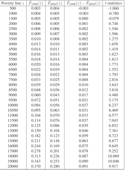
We start using samples from 1996 and 2002 to highlight some hurdles com-monly faced in the analysis of dominance, and thus to emphasize the impor-tance of proper tests for poverty dominance. Table 3 shows the estimated head-count poverty rates bFyear(z) for a grid of poverty lines that lie between $500 and
$20,000. Also note that throughout this illustration we make an arbitrary choice of a maximum possible poverty line z+ equal to $20,000 of equivalent income8.
The estimated differences bF2002(z) − bF1996(z) as well as associated t-statistics for each of these points are also presented. One immediate observation from Ta-ble 3 is that we are unaTa-ble to rank distributions F1996(z) and F2002(z) over the entire range of [$500, $20,000] because the two cumulative distribution functions cross at the lower tails of the distributions. This leads to the emphasis on restricted dominance.
The second observation is that even if we focus on restricted dominance, the estimates of the lower/upper thresholds may vary depending on how many num-bers of points in Z are included in testing differences between two curves. At a 5% significance level, Table 3 reveals poverty dominance of F2002(z) over F1996(z) over a range [$7,000, $20,000] of poverty lines. However, the range of restricted dominance becomes wider as fewer points in Z are evaluated: [$6,000, $20,000] when a grid of 20 points (at intervals of $1,000) is used, and [$4,000, $20,000] when only 10 points (at intervals of $2,000) are used. This suggests that test-ing for poverty dominance should involve testtest-ing for differences in curves over a
8Although arbitrary, the upper bound of $20,000 would seem to be sufficiently reasonably
high to encompass most of the plausible poverty lines for an adult equivalent. To put this into perspective, the commonly used Canadian Low-Income Cutoff (LICO) for an adult in a large city (population size of 500,000 and above) equivalent is about $15,353 (in 2000 dollars).
sufficiently large number of points.
Note that in Table 3 the t-statistics of the difference for each of these points examined take full account of survey design. This is done not only by using sampling weights to compute correctly the point estimates, but also by considering the stratification and the clustering of the survey design to get the standard errors right.
Stratification partitions the population into parts (or strata) that (generally) differ significantly from each other. Sampling then draws information systemat-ically from each of those parts. With stratification, no part of the sampling base goes totally unrepresented in the final sample. Because of this, information from a stratified population leads on average to more precise estimators; a failure to take into account stratification in the computation of standard errors then typi-cally overestimates them.
Clustering (or multi-stage sampling) can generate an inverse bias. Variables of interest (such as incomes) usually vary less within a cluster than between clus-ters. Ceteris paribus, clustering then reduces the informational content provided by a sample and leads to a less informative coverage of the population. Cluster-ing therefore tends to decrease the precision of estimators; failure to take it into account will generally underestimate standard errors.
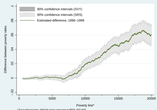
To show the inference impact of testing dominance with and without taking into account the complex survey design of the SLID data, we show differences in distribution functions for 3 pairs of years (1996 minus 2002, 1999 minus 2002, and 1996 minus 1999) in Figures 2, 3 and 4 respectively. The 90% confidence intervals of the estimated differences calculated using survey design (SVY) are designated by dark shading; the confidence intervals without taking account sur-vey design — thus assuming simple random sampling (SRS) — are marked by light shading.
Overall, the confidence intervals are generally wider with an account for sur-vey design than without. That is, ignoring the complexity of the SLID sursur-vey design will usually produce standard errors that are smaller than their real value. Those Figures also reveal however that the impact of ignoring sample design is negligible for the SLID estimators of distribution functions (and therefore for SLID poverty rates), particularly for lower values of z.
It is nevertheless important to stress that such a finding is data-dependent. For most complex surveys, the presumption (and the usual finding) is that the effect of clustering dominates by far the effect of stratification (see for instance Asselin 1984 and Howes and Lanjouw 1998); taking into account survey design often doubles the size of standard errors. That the effect of clustering is roughly undone
by the effect of stratification with the SLID is due to the very fine stratification observed in SLID (an average of around 1,000 strata per sample). Even with the SLID, the net standard error effect varies with the years and the estimators. For instance, complex survey design yields 90% confidence intervals that are visibly (although modestly) different from those obtained under the assumption of SRS for the 1999-2002 comparison (Figure 3), but SVY yields almost identical results to SRS for the 1996-1999 comparison (Figure 4).
We now perform tests of the null of non-dominance that Fearly year(z) ≤
Frecent year(z) against the alternative that Fearly year(z) > Frecent year(z) over a range of $500 (z−) to $20,000 (z+). The results are shown in Table 4 for 3 pairs
of sample years, and for both the minimum t-statistics (with and without survey design, labelled by SRS and SVY respectively) and the empirical likelihood ratio (ELR) approaches as described above. Test statistics are evaluated at each income value observed in the sample over this range. For comparison purposes, column 1 (under “Estimates”) of Table 4 also reports the “crossing” point of the two empir-ical distribution functions, without taking into account the sampling variability of those functions.
Overall, recent years poverty dominate earlier years for a wide range of poverty lines. This is consistent with macro conditions, since 1996 is at the start of a pe-riod of economic recovery that was followed until 2002 by years of expansion. Table 4 also suggests that the estimated range of dominance can vary significantly with the procedures employed. In all cases, it shows that poverty comparison without taking into account sampling variability can largely inflate the range of dominance. This is particularly true in comparing 1996 with 2002 and 1999 with 2002: restricted dominance ranges from [$1704, 20,000$] to [$6879 , 20,000$] and from [$975 , 20,000$] to [$9,562 , 20,000$] respectively SRS sampling vari-ability (under column “SRS”) is imputed to the estimates shown under column “Estimates”. Again, however, the extent to which these differences exist is nec-essarily data-dependent; here the differences are particularly strong for the 1999-2002 comparison.
With respect to tests based on the minimum t-statistics, the results of Table 4 that take full account of survey design (SVY) have larger standard errors and thus narrower ranges of dominance. For instance, we would reject the null of non-dominance of 2002 over 1996 at a 5% significance level for a range of [$6,953, $20,000] with the SVY procedure; we would do this for a range of [$6,879, $20,000] with the SRS procedure. In other words, a failure to take account of survey design results in this case in a modestly $74-wider range of poverty lines
over which we can infer dominance. Table 4 also demonstrates that the effect of ignoring survey design can be data-dependent and sensitive to the significance levels specified. Using a 5% test for a 1999-2002 comparison under SVY as op-posed to SRS decreases by more than $3,600 the range of poverty lines over which dominance can be inferred.
Next we consider test results based on empirical likelihood function (ELR) statistics. As discussed above, this procedure draws inference from bootstrap tests in which the empirical distribution function is drawn from bootstrap sam-ples through a data-generating process that satisfies the null hypothesis of non-dominance. The procedure does not use an asymptotic distribution of the statistics as required in the minimum t-statistics approach. Since the bootstrap test statis-tics that are used here are pivotal, in that their distribution does not depend on unknown parameters, the true size of the test can also be expected to converge more rapidly to the nominal size used.
However, this methodological advantage comes at some cost in terms of com-plexity. This is because, in addition to greater computational time, one needs the drawing of the bootstrap samples to follow the complex survey design of the original survey. This involves following the different procedures and stages (i.e., stratification and clustering) involved in the original sampling of the data (see Section 6.3 for a detailed procedure for applying bootstrap tests). In principle, this is of course a surmountable difficulty. We found, however, that this procedure may be more problematic for complex survey designs that contain many strata and relatively few primary sampling units within each stratum, as is the case for the SLID data9. Bootstrap samples being drawn being replacement, the probability of
drawing repeatedly the same single sampling unit within a small stratum may be relatively large. We find that this event indeed occurs often with the SLID data.
Fortunately, we saw previously (recall Figures 2, 3 and 4) that complex survey design yields confidence intervals with SLID that are close to those obtained under the assumption of simple random sampling. More usefully perhaps, we can com-pare the performance of the bootstrap ELR tests and of the minimum t-statistics under the assumption of simple random sampling with the SLID. We therefore ignore sampling design information in computing the ELR statistics.
The result is reported in the last column of each pair comparison in Table 4. In all cases, bootstrap tests were based on 399 bootstrap samples. In general, the use of ELR statistics shows a relatively modest increase in the ranges of poverty
9There are more than 1,000 strata in each single year of the SLID data we use; within a stratum,
lines over which we may reject the null of non-dominance. At a level of 5%, the bootstrap test for the 1996-2002 comparison leads to a restricted dominance range [$6,876, $20,000] that is slightly wider than the range [$6,953, $20,000] obtained with the asymptotic test (SVY) — namely, an extension of about $77 in the range of poverty lines over which 2002 can be declared to have less poverty. The range extension provided by ELR is slightly larger ($157) for the 1999-2002 comparison, but is even smaller ($17) for the 1996-1999 comparison.
5 Conclusion
Recent years have seen an increased interest in comparing poverty across space and time. Comparing poverty, however, involves making a substantial number of important and difficult methodological choices. Agreement on an official poverty line in Canada has not been possible, and the value and contribution of using poverty aggregation indices that are more ethically acceptable than the traditional headcount ratio have rarely been discussed in Canada.
In view of this, this paper proposes and applies statistical tests for poverty dominance that check for whether poverty comparisons can be made robustly over ranges of poverty lines and classes of poverty indices. The tests are also implemented for the first time in the context of the complex sampling procedures that are typically used by statistical agencies to generate household-level surveys. This helps provide both normative and statistical confidence in ranking two distri-butions in terms of poverty.
The procedures are implemented using the Canadian Survey of Labour and Income Dynamics (SLID). SLID data are drawn from a complex sampling struc-ture based on a stratified, multi-stage design that uses probability sampling. Three years are compared, 1996, 1999 and 2002.
We are unable to rank these years over the entire range of poverty lines [$500, $20,000] (in 2002 dollars) since the cumulative distribution functions cross at the lower tails of the distributions. We are, however, able to infer restricted dominance over ranges that use closer lower and upper thresholds for these ranges. Thus, dominance tests can be used to provide rankings of poverty that are valid (even) over relatively short periods of time and that are robust to the type of measurement choices that have been difficult to make in Canada.
Overall, we find that recent years in Canada poverty dominate earlier years for a relatively wide range of poverty lines. The estimated range of dominance can, however, vary significantly with the procedure that is employed. Estimates of the
critical value of poverty thresholds can depend on how many numbers of points are included in testing differences between two distribution functions; it is therefore find useful to proceed by performing the tests at each observed income point in the samples. More generally, poverty comparisons that fail (as is still often the case) to take into account sampling variability can inflate significantly one’s confidence in making dominance comparisons. This is certainly an important warning for those interested in poverty comparisons for evaluative and/or policy purposes.
Taking full account of survey design (SVY) also leads to larger standard errors and thus to narrower ranges of dominance than (wrongly) assuming simple ran-dom sampling (SRS). Given SLID’s important stratification, this latter effect is, howeverm relatively modest in Canada. But the effect of ignoring survey design can be expected to be highly data-dependent (and to be larger for other types of surveys and for other countries). We find for instance that a 5% test for a 1999-2002 comparison under SVY as opposed to SRS decreases by more than $3,600 the range of poverty lines over which poverty dominance can be inferred. This is an important result given that issues of sampling design have been given little (if any) attention until now by poverty analysts around the world.
Finally, the use of bootstrapped empirical likelihood ratio statistics leads to a relatively modest increase in the ranges of lines over which we may reject the null of non-dominance. This modest increase in power, which can arise from the fact that these bootstrapped statistics are pivotal, is again data specific and could presumably be larger if one were to use smaller-size samples or comparisons across subgroups of the population.
6 Appendix: Stochastic dominance and empirical
likelihood statistics
6.1 Empirical likelihood statistics
Sections 6.1.1 and 6.2 draw significantly from Davidson and Duclos (2006). 6.1.1 Unconstrained likelihood
Let two distributions, A and B, be characterized by their cumulative distribution functions FAand FB. As explained in the paper, distribution B poverty-dominates
A at first order if, for all y ∈ Z, FA(y) > FB(y). Suppose that we have two
NBdenote the sizes of the samples drawn from distributions A and B respectively. Let YAand YBdenote respectively the sets of (distinct) realizations in samples A and B, and let Y be the union of YA and YB. For K = A, B, let yK
t be a point in YK and wK
t be the sum of the sampling weights associated to ytK, relative to the overall sum in the sample of K. When we look at poverty among Canadian individuals in Section 4 above, these sample weights are given by the product of household sampling weights and household size. The empirical distribution functions (EDFs) of the samples can then be defined as follows. For any y ∈ Y , we have ˆ FK(y) = X yK t ∈YK wK t I(yKt ≤ y), (5)
where I(·) is an indicator function, with value 1 if the condition is true, and 0 if not. If it is the case that ˆFA(y) > ˆFB(y) for all y ∈ Z, we say that we have first-order poverty-dominance of A by B in the sample.
For a given sample, the parameters pK
t of the empirical likelihood for the sam-ple of K are the probabilities associated with each point yK
t in YK. The empirical loglikelihood function (ELF) is then the sum of the logarithms of these probabili-ties. The ELF is hence NKP
yK
t ∈YKw K
t log pKt . In the absence of constraints, the ELF is maximized by solving the problem
max pK t NK X yK t ∈YK wK t log pKt subject to X yK t ∈YK pK t = 1, (6)
for which the solution is pK
t = wKt for all t. The maximized ELF is then NK P
twtKlog wtK. With two samples, A and B, the maximized ELF is therefore
NA X yA t∈YA wtAlog wtA+ NB X yB t ∈YB wtBlog wBt . (7)
The null hypothesis we wish to consider is that B does not poverty-dominate
A, that is, that there exists at least one y ∈ Z such that FA(y) ≤ FB(y). If there
is a y ∈ Z such that ˆFA(y) ≤ ˆFB(y), there is non-dominance in the samples, and, in such cases, we do not wish to reject the null of non-dominance. If there is dominance in the samples, then the constrained estimates must be different from the unconstrained ones, and the empirical loglikelihood maximized under the constraints of the null is smaller than the unconstrained maximum value.
6.1.2 Constrained likelihood
In order to maximise the ELF under the constraint of the null, we begin by com-puting the maximum where, for a given y ∈ Z, we impose the condition that
FA(y) = FB(y). We then choose for the constrained maximum that value of y
that gives the greatest value of the constrained ELF.
For given y, the constraint we wish to impose can be written as X yA t ∈YA pA tI(ytA≤ y) = X yB s∈YB pB sI(ysB ≤ y). (8)
The maximisation problem can thus be stated as follows: max pA t,pBt X yA t ∈YA NAwtAlog pAt + X yB t ∈YB NBwtBlog pBt (9) subject to X yA t ∈YA pAt = 1, X yB t ∈YB pBt = 1, X yA t ∈YA pAt I(ytA≤ y) = X yB t ∈YB pBt I(ytB ≤ y).(10) Letting NA+ NB = N, NK(y) = P
tNKwKt I(ytK ≤ y) and MK(y) = NK −
NK(y), the probabilities that solve this problem can be written as
pA t = NAwA t I(yAt ≤ y) ν + NAwA t (1 − I(ytA≤ y)) λ (11) and pB t = NBwB t I(ytB ≤ y) N − ν + NBwB t (1 − I(yBt ≤ y)) N − λ (12) with ν = NNA(z) NA(z) + NB(z) (13) and λ = NMA(z) MA(z) + MB(z). (14)
We may use this to express the value of the constrained ELF as P
tNAwtAlog(NAwtA) + P
sNBwBs log(NBwBs)
−NA(z) log ν − MA(z) log λ − NB(z) log(N − ν) − MB(z) log(N − λ). (15) Twice the difference between the unconstrained maximum in (7) and the con-strained maximum in (15) is an empirical likelihood ratio (ELR) statistic at z.
We now see how to use the probabilities in (11) and (12) in order to test the hypothesis of non-dominance.
6.2 Testing restricted dominance with simple random sampling
To test for restricted dominance, a natural way to proceed, in cases in which there is dominance in the sample, is to seek an interval [ˆz−, ˆz+] over which one canreject the hypothesis
max
z∈[ˆz−,ˆz+]FB(z) − FA(z) ≥ 0. (16)
As the notation indicates, ˆz− and ˆz+ are random, being estimated from the
sample.
We have at our disposal two test statistics to test the null hypothesis that dis-tribution B does not dominate disdis-tribution A, the ELR statistic given by (6) and (13) and the t-ratio tmin statistic given by (3). Again, it is only when there is dominance in the sample that there is any possible reason to reject the null of non-dominance. Then the minimum t statistic (which will be positive if there is dominance in the sample) can be found by minimizing t(y) over Z – this gives ˜y
and t(˜y). There is no loss of generality in restricting the search for the maximizing y to the intersection of Y and Z since t(y) is constant between sorted elements of
Y TZ.
Since the EDFs are the distributions defined by the probabilities that solve the problem of the unconstrained maximisation of the empirical loglikelihood func-tion, they define the unconstrained maximum of that function. The constrained empirical likelihood estimates of the CDFs of the two distributions can be written as ˜ FK(z) = X yK t ∈YK pK t I(yKt ≤ z), (17)
K = A, B, where the probabilities pK
t are given by in (11) and (12) with y = ˜y. The distributions ˜FA and ˜FB are on the frontier of the null hypothesis of non-dominance, and they represent those distributions contained in the null hypothesis that are closest to the unrestricted EDFs by the criterion of the empirical likeli-hood.
The minimum over Z of the asymptotic t statistic is asymptotically pivotal for the null hypothesis that the distributions A and B lie on the frontier of non-dominance of A by B. This means that we can use the bootstrap to perform tests that should benefit from asymptotic refinements in finite samples – see Beran (1988). On this frontier, the empirical likelihood ratio statistic is asymptotically pivotal, by which it is meant that they have the same asymptotic distribution for all configurations of the population distributions that lie on the frontier.
6.3 Test for poverty dominance with complex survey design
The following outlines a procedure for the use of the above tmin and empirical likelihood statistics with samples drawn using stratification and multi-stage sam-pling. Such a survey design was followed by Statistics Canada for the Canadian SLID data used in this paper.1. We first set a value for z−and z+; this defines Z.
2. We then compute the asymptotic t-ratio statistic of the difference FA(z) −
FB(z) in the distribution functions of two populations at each value of Z that is observed in the samples. This is done taking into the sampling design (stratification and clustering) of the survey – see for instance Chapter 16 and Section 16.5 in Duclos and Araar (2006).
3. We then find the point ˜y at which this t-ratio is minimized. Denote by t0the
value of this t-ratio.
4. We then compute the probabilities pA
t and pBt using (11) and (12) at y = ˜y.
5. We then bootstrap β samples from the two distributions now defined by
these probabilities pA
t and pBt . Each of these β samples is a combination of two samples, one drawn with replacement from A and the other drawn with replacement from B. In drawing such bootstrap samples, we follow the sampling design of the original surveying process. For this, we must therefore take into account the clustering (the different levels of sampling) and stratification of the surveys.
Say:
• that our survey of A contains SAstrata, s = 1, ..., SA;
• that, within a stratum s, a number CA
s of primary sampling units have been drawn, with the set of such primary sampling units being given by cA
s;
• that within each primary sampling unit c1 in the set cA
s, a number of final sampling units CA
s,c1 has been drawn, with the set of such final sampling units being given by cA
s,c1.
Denote by πA
s,u the relative probability of primary sampling unit u being drawn from the set of all of the primary sampling units that belong to stra-tum s; this is given by
πA s,u= P t∈cA s,up A t P t∈cA s p A t , u ∈ cA s. (18) Similarly, define πA
s,c1,u as the relative probability of final sampling unit u
being drawn from the set of all of the final sampling units that belong to the primary sampling unit c1 of stratum s:
πA s,c1,u = pA u P t∈cA s,c1p A t , u ∈ cA s,c1. (19)
6. For each of b = 1, ..., β, the bootstrap process then consists of two steps:
(a) from each stratum s, select randomly CA
s primary sampling units with replacement from the original sample A, each with probability πA
s,u;
(b) from each primary sampling unit c1 selected above, select randomly
CA
s,c1 final sampling units with replacement from the set of final sam-pling units cA
s,c1, each with probability πs,c1,uA . Repeat the process for all β samples.
7. For each bootstrap b, calculate the minimum t-statistic as in points 2 and 3 on page 22 above, but using as weights those that correspond to the empir-ical likelihood probabilities of being selected in the sample, namely, those given by the πK of (18) and (19).
8. Once this has been done for B bootstraps, compute the proportion of the
B minimum t-statistics that exceed t0. If this proportion is below a
reason-able significance level (say 5%), then reject the null of non-dominance and accept the alternative hypothesis of dominance.
Table 1: Sensitivity of poverty comparisons to choice of poverty indices and poverty lines
Distribution A Distribution B First individual’s income 0.4 0.6 Second individual’s income 1.1 0.9 Third individual’s income 2 2
P (0.5; 0) 0.33 0
P (1; 0) 0.33 0.66
P (1; 1) 0.2 0.166
Table 2: Sensitivity of differences in poverty to choice of indices Individuals Indices
Distributions First Second P (1; α = 0) P (1; α = 1) P (1; α = 2)
A 0.25 2 0.5 0.375 0.28125
B 0.5 2 0.5 0.25 0.125
Table 3: Difference between poverty incidence curves for 1996 and 2002 for var-ious income-based poverty lines. Incomes are equivalent incomes; squared-root household size is used as equivalence scale. t-statistics take full account of survey
design.
Poverty line z Fˆ1996(z) Fˆ2002(z) Fˆ1996(z) − ˆF2002(z) t-statistics
500 0.003 0.004 -0.001 -1.060 1000 0.004 0.005 -0.001 -0.780 1500 0.005 0.005 0.000 -0.079 2000 0.006 0.005 0.001 0.748 2500 0.008 0.006 0.002 1.546 3000 0.009 0.007 0.002 1.506 3500 0.010 0.008 0.002 1.275 4000 0.013 0.010 0.003 1.658 4500 0.014 0.011 0.002 1.419 5000 0.016 0.013 0.003 1.623 5500 0.018 0.014 0.004 1.813 6000 0.020 0.016 0.004 1.773 6500 0.022 0.019 0.004 1.552 7000 0.026 0.022 0.004 1.793 7500 0.033 0.025 0.008 2.816 8000 0.039 0.029 0.010 3.643 8500 0.048 0.036 0.012 3.818 9000 0.060 0.043 0.017 4.480 9500 0.072 0.051 0.021 5.175 10000 0.084 0.056 0.027 6.237 10500 0.095 0.063 0.031 6.469 11000 0.104 0.070 0.033 6.577 11500 0.114 0.076 0.037 7.043 12000 0.125 0.086 0.039 6.852 13000 0.150 0.104 0.046 7.361 14000 0.182 0.123 0.059 8.723 15000 0.211 0.148 0.063 8.677 16000 0.244 0.169 0.075 9.645 17000 0.278 0.201 0.078 9.252 18000 0.313 0.226 0.087 10.069 19000 0.343 0.253 0.090 10.046 20000 0.370 0.280 0.091 9.917
T able 4: Ranges (in $) of dominance of columns ov er ro ws. Incomes are equi valent incomes. Squared-root house-hold size is used as equi valence scale. T ests at 5% significance le vel. T esting procedures are based on simple comparisons of sample estimates (Estimates), on t-statistics assuming simple random sampling design (SRS), on t-statistics taking full account of surv ey design (SVY), and on empirical lik elihood ratio statistics assuming simple random sampling when dra wing bootstrap samples (ELR). 1999 2002 Estimates SRS SVY ELR Estimates SRS SVY ELR 1996 7,041 8,288 8,288 8,271 1,704 6,879 6,953 6,584 20,000 20,000 20,000 20,000 20,000 20,000 20,000 20,000 1999 975 9,562 13,179 8,441 20,000 20,000 20,000 20,000
Figure 1: First-order po verty dominance
F(y)
y
F (y)
F (y)
B Az
+z
++z
-Figure 2: Differences in distribution functions, 1996 minus 2002, with 90% con-fidence intervals, with (SVY) and without (SRS) taking account of survey design
in the computation of the standard errors
−.02 0 .02 .04 .06 .08 .1
Difference between poverty rates
0 5000 10000 15000 20000
Poverty line* 90% confidence intervals (SVY) 90% confidence intervals (SRS) Estimated difference, 1996−2002
Figure 3: Differences in distribution functions, 1999 minus 2002, with 90% con-fidence intervals, with (SVY) and without (SRS) taking account of survey design
in the computation of the standard errors
−.02 0 .02 .04 .06 .08 .1
Difference between poverty rates
0 5000 10000 15000 20000
Poverty line* 90% confidence intervals (SVY) 90% confidence intervals (SRS) Estimated difference, 1999−2002
Figure 4: Differences in distribution functions, 1996 minus 1999, with 90% con-fidence intervals, with (SVY) and without (SRS) taking account of survey design
in the computation of the standard errors
−.02 0 .02 .04 .06 .08 .1
Difference between poverty rates
0 5000 10000 15000 20000
Poverty line* 90% confidence intervals (SVY) 90% confidence intervals (SRS) Estimated difference, 1996−1999
References
ANDERSON, G. (1996): “Nonparametric Tests of Stochastic Dominance in
Income Distributions,” Econometrica, 64, 1183–93.
ASSELIN, L.-M. (1984): Techniques de sondage avec applications à
l’Afrique, Centre canadien d’études et de coopération internationale,
CECI/Gaëtan Morin.
ATKINSON, A. (1987): “On the Measurement of Poverty,” Econometrica,
55, 749 –764.
BARRETT, G. AND S. DONALD (2003): “Consistent Tests for Stochastic
Dominance,” Econometrica, 71, 71–104.
BEACH, C. AND R. DAVIDSON (1983): “Distribution-Free Statistical
In-ference with Lorenz Curves and Income Shares,” Review of Economic
Studies, 50, 723–35.
BERAN, R. (1988): “Prepivoting test statistics: A bootstrap view of
asymp-totic refinements,” Journal of the American Statistical Association, 83, 687–697.
BISHOP, J., J. FORMBY, AND P. THISTLE (1992): “Convergence of the
South and Non-South Income Distributions, 1969-1979,” American
Eco-nomic Review, 82, 262–72.
CHEN, W.-H. (2008): “Comparing Low Income of Canada’s
Re-gions: A Stochastic Dominance Approach,” Catalogue No.
75F0002MIE2008006-No. 6, Statistics Canada, Ottawa.
DARDANONI, V. AND A. FORCINA (1999): “Inference for Lorenz Curve
Orderings,” Econometrics Journal, 2, 49–75.
DAVIDSON, R. AND J.-Y. DUCLOS (2000): “Statistical Inference for
Stochastic Dominance and for the Measurement of Poverty and Inequal-ity,” Econometrica, 68, 1435–64.
——— (2006): “Testing for Restricted Stochastic Dominance,” Working Paper 06-09, CIRPEE.
DUCLOS, J.-Y. AND A. ARAAR (2006): Poverty and Equity
Measure-ment, Policy, and Estimation with DAD, Berlin and Ottawa: Springer
FOSTER, J., J. GREER, ANDE. THORBECKE (1984): “A Class of
Decom-posable Poverty Measures,” Econometrica, 52, 761–776.
FOSTER, J.ANDA. SHORROCKS(1988a): “Poverty Orderings,”
Economet-rica, 56, 173–177.
——— (1988b): “Poverty Orderings and Welfare Dominance,” Social
Choice Welfare, 5, 179–98.
GILES, P. (2004): “Low Income Measurement in Canada,” Catalogue No.
75F0002MIE2004011-No. 11, Statistics Canada, Ottawa.
HOWES, S. (1993): “Restricted Stochastic Dominance: A Feasible
Ap-proach to Distributional Analysis,” Tech. rep., STICERD.
HOWES, S. AND J. LANJOUW (1998): “Does Sample Design Matter for
Poverty Rate Comparisons?” Review of Income and Wealth, 44, 99–109.
HUMAN RESOURCES AND SOCIAL DEVELOPMENT CANADA (2006):
“Low Income in Canada: 2000-2002 using the Market Basket Measure,” Tech. Rep. SP-628-05-06E, Ottawa.
KAUR, A., B. L. S. PRAKASA RAO, AND H. SINGH (1994): “Testing for
Second-Order Stochastic Dominance of Two Distributions,”
Economet-ric Theory, 10, 849–66.
LINTON, O., E. MAASOUMI,ANDY.-J. WHANG(2005): “Consistent
Test-ing for Stochastic Dominance under General SamplTest-ing Schemes,”
Re-view of Economic Studies, 732, 735–765.
OSBERG, L. (2002): “Trends in poverty: The UK in international
perspec-tive – how rates mislead and intensity matters,” Working Paper 2002-10, Institute for Social and Economic Research, University of Essex, Colch-ester.
PICOT, G., F. HOU, AND S. COULOMBE (2007): “Chronic Low Income
and Low-income Dynamics among Recent Immigrants,” Catalogue No. 11F0019MIE2007294-No. 294, Statistics Canada, Ottawa.