Testing Optimal Punishment Mechanisms Under Price Regulation: the Case of the Retail Market for Gasoline

Texte intégral

(1)2003s-57. Testing Optimal Punishment Mechanisms Under Price Regulation: the Case of the Retail Market for Gasoline Robert Gagné, Simon van Norden, Bruno Versaevel. Série Scientifique Scientific Series. Montréal Septembre 2003. © 2003 Robert Gagné, Simon van Norden, Bruno Versaevel. Tous droits réservés. All rights reserved. Reproduction partielle permise avec citation du document source, incluant la notice ©. Short sections may be quoted without explicit permission, if full credit, including © notice, is given to the source..

(2) CIRANO Le CIRANO est un organisme sans but lucratif constitué en vertu de la Loi des compagnies du Québec. Le financement de son infrastructure et de ses activités de recherche provient des cotisations de ses organisationsmembres, d’une subvention d’infrastructure du ministère de la Recherche, de la Science et de la Technologie, de même que des subventions et mandats obtenus par ses équipes de recherche. CIRANO is a private non-profit organization incorporated under the Québec Companies Act. Its infrastructure and research activities are funded through fees paid by member organizations, an infrastructure grant from the Ministère de la Recherche, de la Science et de la Technologie, and grants and research mandates obtained by its research teams. Les organisations-partenaires / The Partner Organizations P ARTENAIRE MAJEUR . Ministère du développement économique et régional [MDER] P ARTENAIRES . Alcan inc. . Axa Canada . Banque du Canada . Banque Laurentienne du Canada . Banque Nationale du Canada . Banque de Montréal . Banque Royale du Canada . Bell Canada . Bombardier . Bourse de Montréal . Développement des ressources humaines Canada [DRHC] . Fédération des caisses Desjardins du Québec . Gaz Métropolitain . Hydro-Québec . Industrie Canada . Ministère des Finances [MF] . Pratt & Whitney Canada Inc. . Raymond Chabot Grant Thornton . Ville de Montréal . École Polytechnique de Montréal . HEC Montréal . Université Concordia . Université de Montréal . Université du Québec à Montréal . Université Laval . Université McGill ASSOCIÉ À : . Institut de Finance Mathématique de Montréal (IFM2 ) . Laboratoires universitaires Bell Canada . Réseau de calcul et de modélisation mathématique [RCM2 ] . Réseau de centres d’excellence MITACS (Les mathématiques des technologies de l’information et des systèmes complexes) Les cahiers de la série scientifique (CS) visent à rendre accessibles des résultats de recherche effectuée au CIRANO afin de susciter échanges et commentaires. Ces cahiers sont écrits dans le style des publications scientifiques. Les idées et les opinions émises sont sous l’unique responsabilité des auteurs et ne représentent pas nécessairement les positions du CIRANO ou de ses partenaires. This paper presents research carried out at CIRANO and aims at encouraging discussion and comment. The observations and viewpoints expressed are the sole responsibility of the authors. They do not necessarily represent positions of CIRANO or its partners.. ISSN 1198-8177.

(3) Testing Optimal Punishment Mechanisms Under Price Regulation: the Case of the Retail Market for Gasoline Robert Gagné,* Simon van Norden,† Bruno Versaevel‡ Résumé / Abstract Nous analysons les effets de la présence d’un prix plancher dans le marché de la vente au détail de l’essence. D’un point de vue théorique, nous supposons un modèle à la Bertrand où au départ les firmes font implicitement collusion en demandant le prix de monopole. Lorsqu’une firme dévie de cette stratégie, les firmes concurrentes modifient également leur stratégie en punissant la firme déviante par des prix plus bas (guerre de prix) avant de retourner au prix de collusion. L’introduction d’une réglementation de type prix plancher dans le marché de la vente au détail de l’essence au Québec en 1996 procure une expérience naturelle pour tester le modèle théorique. Nous utilisons un modèle de type «Markov Switching» avec deux états latents afin d’identifier simultanément les périodes de prix collusifs et de guerres de prix et d’estimer les paramètres caractérisant chacun de ces états. Les résultats montrent que l’introduction d’un prix plancher réduit l’intensité des guerres de prix mais accroît leur durée anticipée. Mots clés : réglementation des prix, jeu à la Bertrand, modèle de Markov, prix de l’essence.. We analyse the effects of a price floor on price wars in the retail market for gasoline. Our theoretical model assumes a Bertrand oligopoly supergame in which firms initially collude by charging the monopolistic price. Once firms detect a deviation from this strategy, they switch to a lower price for a punishment phase (a “price war” before returning to collusive prices. In 1996, the introduction of a price floor regulation in the Quebec retail market for gasoline serves as a natural experiment with which to test our model. We use a Markov Switching Model with two latent states to simultaneously identify the periods of price-collusion/pricewar and estimate the parameters characterizing each state. Results show that the introduction of the price floor reduces the intensity of price wars but raises their expected duration. Keywords: price regulation, oligopoly supergame, Markov switching model, gasoline prices. Codes JEL : L13, L81, C32.. *. Corresponding author. Address: Institut d’économie appliquée, HEC Montréal, 3000 chemin de la Côte-SainteCatherine, Montréal, Québec, Canada H3T 2A7. Email: robert.gagne@hec.ca. † HEC Montréal and CIRANO. ‡ EM Lyon and GATE..

(4) 1. Introduction. The behaviour of gasoline retail prices has long been and still is the object of fierce public debates. Given the importance of this product for the consumers and the apparently “suspect” behaviour of the integrated oil companies (the “majors”), many jurisdictions have regulated aspects of gasoline retailing. In some U.S. states, refiners are forbidden to operate retail outlets. Different types of price regulations are also enforced in several U.S. states and Canadian provinces. In this paper, we provide evidence of the effects of the provincial price floor regulation on the behaviour of gasoline retail prices in Montreal, the largest market in the province of Quebec.. Following a severe price war during the summer of 1996, the Quebec provincial government responded to the lobbying of independent gasoline retailers by establishing a price floor in December 1996. The floor was introduced to limit the severity of price wars which, majors according to the independent retailers, were an evidence of a predatory behaviour by the integrated. The price floor was therefore viewed as a form of market protection for independent retailers which would help to maintain a sufficient level of competition in the market. The floor is computed weekly and regionally as the sum of the wholesale (rack) price, transportation costs and taxes, and is the only type of economic regulation in the Quebec’s retail market of gasoline.. The introduction of this price regulation provides a natural experiment from which a model of price behaviour involving punishment mechanisms can be tested. From a theoretical point of view, we assume that gasoline retail prices behave according to a Bertrand oligopoly supergame in which firms initially collude by charging the monopolistic price. 1 Once firms detect a deviation from this strategy, they switch to a lower price for a punishment phase (a “price war”) before reverting to the collusive price. We compare the optimal punishment prices in two cases: 1) when the price is allowed to fall below the marginal cost (which corresponds in our case to the price floor), and 2). 1. Collusion is defined here as implicit collusion and should not be interpreted as explicit agreements or other kinds of coordination between firms in the market.. 1.

(5) when regulation prohibits pricing below marginal cost. When the level of product differentiation is relatively high, we find that optimal punishment prices are the same with or without regulation and last only one period. When the level of product differentiation is lower (which is the case for gasoline), the price floor is binding and price wars last longer.. Our model gives testable predictions about the behaviour of prices without and with regulation. In this paper, we test whether market prices behave in a manner consistent with the model. Such consistency would support a class of price models which do not assume any kind of coordination or explicit collusion between firms in the studied market.. To test our model, we use a Markov Switching Regression framework with two latent states to simultaneously identify the periods of price-collusion/price-war and estimate the parameters characterizing each state. Consistent with the model, we allow regulation to influence both the state-conditional prices and the expected duration of each state. The switching regression is then estimated on weekly data for retail gasoline prices in Montreal from 1994 to 2001.. Section 2, below, presents the Bertrand oligopoly supergame with price regulation. The empirical model and data are described in Section 3. The results are discussed in Sectio n 4, and Section 5 presents concluding remarks.. 2. Theoretical Model. In this section, we extend Lambertini and Sasaki’s (2002) model to an oligopoly setting in which identical firms in. N = {1, K , n} maximize intertemporal profits by. simultaneously and non-cooperatively choosing prices in an infinitely repeated game over. t = 1, 2, K , ∞. The discount factor δ = 1 /(1 + r ) , where r is the single period interest rate, is common to all firms. Every consumer has the same time-invariant utility function. 2.

(6) n  1 n U (q , I ) = ∑ q i −  ∑ qi2 + 2γ ∑ qi q j  + I , 2  i =1 i =1 i≠ j . which is quadratic in the consumption of q-products, with q = (q1 , K, q n ) , and linear in the consumption of the composite I-good. 2 The parameter γ ∈ (0,1) measures product substitutability as perceived by consumers. If γ → 0 , each firm has monopolistic market power, while if γ → 1 , the products are perfect substitutes. Consumers maximize utility subject to the budget constraint. ∑p q i. i. + I ≤ m , where m denotes income, p i is the. price of product i, and the price of the composite good is normalized to one. By symmetry, we have. ∑. j ≠i. q j = (n − 1)q j . The first-order condition for the optimal. consumption of product i yields a linear inverse demand function p i = 1 − q i − γ ( n − 1)q j ,. j ≠ i . The demand for product i in each period is. qi ( p) =.  (1 + γ (n − 2)) γ (n − 1)  1  1 − pi + p j , 1 + γ (n − 1)  1 −γ 1−γ . and q = (q1 , K, q n ) is such that q i ( p) ≥ 0 for product quantities to make economic sense. In this model, by “price” we actually refer to the difference between the price and a constant unit cost of production c ∈ [0,1] , so that firm i’s profit in the stage game is. p i qi , for all i. In the absence of regulation p i ≥ −c , otherwise the regulation constraint p i ≥ p R applies, where p R is a price floor. In the context of the regulated market for gasoline under scrutiny, we impose p R = 0 .. A strategy profile is a set of available prices. They include a collusive price, which yields joint profit maximization, and a punishment price, which leads to low profits for all firms. In the multi-stage game, a firm’s price strategies may vary from period to period. 2. The utility function is adapted from Häckner (2000), in which quantities q i are multiplied by a parameter a i that is a measure of the distinctive quality of each variety i. Following Lambertini and Sasaki (2002), here we exclude vertical product differentiation between firms by assuming thata i = 1 , for all i ∈ N .. 3.

(7) A price path. {p t }∞t =1. is defined as an infinite sequence of n-dimensional price vectors. charged by firms i = {1, K , n} in each period t. Now suppose that all firms charge the same high monopolistic price p H in a first period. Each firm then has an incentive to lower its own price slightly to capture a larger market share and thereby increase individual profits at every other firms’ expense. Let exactly one firm deviate from the collusive strategy in, say, period two. Then the choice of a low punishment price p L in the third period by all firms penalizes the free-rider. After one (or more) period(s) of price war, all firms may return to collusive profits by charging the high price again in all future periods. This describes a particular price path.. Henceforth, we refer to the following three definitions. A punishment mechanism is symmetric if all firms charge the same price in any given period. A symmetric punishment mechanism is an equilibrium if all firms find it profitable to charge p H whenever the price path calls for them to do so, and to charge p L whenever the price path calls for them to do so. A symmetric equilibrium punishment mechanism is optimal if all other price paths require a higher discount factor to sustain collusion.. In real-world markets, punishment mechanisms implemented over more than one period may be non-stationary. In this model, the most severe punishment prices are assumed to apply in early periods. The objective is to look for a characterization of optimal punishment mechanisms for all degrees of product differentiation and all numbers of firms in two cases : 1) when the price is allowed to fall below the marginal cost (i.e.,. p i ≥ −c ), 2) when regulation imposes a price floor equal to the marginal cost (i.e., p i ≥ p R ≡ 0 ).. ¦ Without regulation. In the absence of regulation, the price can plunge below zero in a price-war period. Consider a price path with a two-phase profile. {p L , p H },. with. p L < p H . Assume that firms initially follow the collusive path p H . After t periods of collusion, if any deviation from p H by any firm i is detected, all n firms switch to the. 4.

(8) punishment phase p L at period t + 1. After one period of punishment, if any deviation from p L by any firm in N is detected, the punishment phase restarts, otherwise all firms convert to the initial collusive path p H forever. We know from Abreu (1986) that, in order for this symmetric 1-period punishment mechanism to be an equilibrium, the incentive compatibility conditions are. π d ( p H ) − π ( p H ) ≤ δ [π ( p H ) − π ( p L )],. (1). π d ( p L ) − π ( p H ) ≤ δ [π ( p H ) − π ( p L )],. (2). where π ( p ) denotes each firm’s profit when all firms charge p, and π d ( p ) is firm i’s maximum profit from a one-shot deviation from the price p. The first condition says that the incentive for the initial deviation must be smaller than what is lost due to the punishment phase. The second condition says that the incentive to deviate from the punishment phase must be smaller than the loss incurred by prolonging the punishment by one more period. We look for an optimal punishment price p L and the threshold level of the discount factor δ (γ ) such that, if p L is prescribed and δ ≥ δ (γ ) , then firms can sustain collusion at p H . To do that, we impose conditions (1 – 2) to hold with strict equalities, then set p H = 1 / 2 (the monopolistic price) and solve the system with respect to p L and δ . 3 Because non-negativity constraints on product quantities bind over different ranges of the differentiation parameter, we find three different solutions. ( p L , δ (γ )) as a function of γ over the three intervals (0,γ ′) , [γ ′, γ ′′) , [γ ′′,1) , with. γ ′=. 3. 1+ 3 3 5 +5 and γ ′ = . n+ 3 2n + 3( 5 + 1). This follows Abreu (1986), who proves, in a more general context, that if there exists a price p L and a. δ (γ ) which satisfy the system of simultaneous conditions (1 – 2) with strict equalities, then there is no punishment price which can sustain collusion at price p H for any δ < δ (γ ) . In that sense, p L is optimal. discount factor. 5.

(9) The computation of solutions and their algebraic expressions are detailed in the appendix.. ¦ With regulation. When a price floor is introduced, a non-negativity constraint on each firm’s price applies. Consider a price path with a three-phase profile {p R , p L , p H }, with. p R ≤ p L < p H . Assume that firms initially follow the collusive path p H . After t periods of collusion, if any firm charges less than p H , all n firms switch to a l-period punishment phase p L, z at periods t + z , where z = 1,K , l , with p L , z = p R for z = 1, K , l − 1 , and th p L, l = p L in the l period. During the punishment phase, after z periods, if any deviation. from p L, z by any firm in N is detected, the punishment phase restarts from p L,1 at period. t + z + 1 . After l periods of punishment, all firms convert to the initial collusive path p H for ever. This means that the most severe feasible (i.e. constrained by regulation) punishment price applies during l − 1 periods, followed by a more lenient (and endogenously determined) punishment price in the final period. We know from Lambertini and Sasaki (2002) that in order for this symmetric l-period punishment mechanism to be an equilibrium, the incentive compatibility conditions are. π d ( p H ) − π ( p H ) ≤ δ l [π ( p H ) − π ( p L, l )] + [δ (1 − δ l ) /(1 − δ )][π ( p H ) − π ( p R )], π d ( p R ) − π ( p R ) ≤ δ l [π ( p H ) − π ( p L,l )] + δ l −1 [π ( p L ,l ) − π ( p R )],. (3) (4). These conditions generalize expressions (1 – 2) to the multiple-period case. For a given l, we look for an optimal lth-period punishment price p L,l and the corresponding threshold level of the discount factor δ (γ ) such that, if p L,l is prescribed and δ ≥ δ (γ ) , then firms can sustain collusion at p H . To do that, we proceed as above by imposing conditions (3 – 4) to hold with strict equality, then we set p H = 1 / 2 and solve the system with respect to. p L,l and δ .. 6.

(10) Denote by ( p L,1 , δ (γ )) the single-period solution (that is, l = 1 ). We find that. p L,1 > p R ≡ 0 if and only if γ < γ 1 , where the latter threshold value is such that. γ1 =. 2 < γ ′ < γ ′′ . n +1. (5). The computation of γ 1 , together with its comparison to γ ′ and γ ′′ , are detailed in the appendix. There it is shown that when the products are sufficiently close substitutes, the price floor renders the single-period punishment impracticable. Since the threshold value. γ 1 decreases when n increases, the price-floor regulation is most effective when the number of firms is high. This does not imply that collusion is not sustainable when the price floor is binding. When the toughest single-period punishment price admissible under regulation ( p R ) is not sufficiently low to make each firm indifferent between deviating from the penal phase and complying with it, the punishment can be made tougher by charging a punishment price p L, 2 in a second period. By the same token, when p L, 2 = p R is not sufficiently low deter deviation from the collusive price, the punishment can be made tougher by charging a price p L,3 in a third period. This incremental logic applies until the determination of a lth-period punishment price p L,l , and a discount factor δ , which are such that the two incentive compatibility conditions hold with equality. More precisely, if γ ≥ γ 1 and l ≥ 2 , distinct solutions ( p L,l , δ (γ )) exist as a function of γ belonging to one of the intervals [γ 1 , γ 2 ), [γ 2 , γ 3 ), K, [γ l −1 ,γ l ) , and are such that p L,1 = K = p L,l −1 = p R and p L, l ∈ [ p R , p H ] , with γ 1 < γ 2 < K < γ l and. lim l → ∞ γ l = 1 . The existence of γ 1 , as displayed in (5), leads to two related theoretical implications. First, the regulation should be ineffective (ceteris paribus) in the event of a price war when product varieties are highly differentiated, whereas the price floor should be binding in a price war when product varieties are sufficiently close substitutes. Second,. 7.

(11) the regulation can be ineffective in the event of a price war when the number of firms is sufficiently small on the relevant markets, whereas the price floor should be binding (ceteris paribus) in a price war when sellers are many. As urban retail markets for gasoline are typically characterized by highly substitutable products and a large number of outlets, this environment should enable us to test the following empirical implication: when a price war occurs, the duration of punishment should be shorter without regulation than when a price floor applies. The econometric model described in the next section enables us to test this prediction.. 3. Econometric Implementation. Data and Variables. Retail price data (Pt) have been provided by M.J. Ervin Inc., a Calgary-based firm which conducts a weekly survey on gasoline retail prices in all major Canadian markets. In each market surveyed, retail prices are collected by gasoline grade using a sample of selfservice gas stations. Whenever possible, the same stations are surveyed each week. In the Montreal market, the survey covers approximately 20 stations. For our analysis, we use the average retail price for unleaded regular gasoline computed from all stations in the Montreal survey. Our data cover the 1994-2001 period (416 weekly observations). Our analysis is limited to the price of unleaded regular gasoline as retail prices for all other grades follow unleaded regular gasoline prices exactly.. Wholesale prices (Wt) have also been provided by M.J. Ervin. Those prices are “rack” prices (excluding taxes) posted everyday at wholesale distribution outlets. As for retail prices, we used the average (unweighted) weekly wholesale price computed from posted prices. No transportation costs are considered given the proximity of the retail market to the different wholesale distribution outlets.. In our empirical analysis, we use retail margins (Mt) rather than prices in order to eliminate price effects coming from the wholesale market and thereby concentrate on. 8.

(12) retail market effects. Retail margins are computed as retail prices in week t minus wholesale prices in week t − 1 to reflect the fact that retail prices may not respond instantly to changes in wholesale prices due to the carrying of retail inventories.. Another variable included in the empirical analysis is the number of retail outlets in the market at each period (Nt). This is measured by a survey conducted every two months by Kent Marketing in the major markets in Canada. The number of retail outlets is assumed to be constant between survey dates. The number of outlets is used here as a proxy for the level of product differentiation in the market (i.e. location). As the number of outlets increases for given market size, the level of differentiation is assumed to decrease because the average distance between outlets (the main cause of differentiation in gasoline retailing) is also decreasing. This can cause products served by different outlets to be sufficiently substitutable from the viewpoint of gasoline buyers, in the sense that. γ > γ 1 , with γ 1 as in (5).. Finally, our empirical analysis includes a regulation dummy (Rt) equal to 0 until the price floor regulation was introduced during the last week of December 1996, and equal to 1 thereafter.. Table 1 presents descriptive statistics for all our variables. Figure 1 shows the evolution of retail margins over time.. Table 1 Descriptive Statistics. Variable. Mean. Minimum. Maximum. Price : Pt (¢/litre). 28.7738. 15.4000. 49.7000. Wholesale price: Wt (¢/litre). 24.3781. 13.7250. 42.8250. Margin : Mt (¢/litre). 4.4176. -6.6500. 12.5000. 1104. 951. 1293. 0.6274. 0. 1. Number of outlets : Nt (#) Regulation : Rt (0,1). 9.

(13) Figure 1. Econometric Model. To assess the relevance of the model presented in Section 2 for the behaviour of the retail gasoline margins, we need to allow for the structural relationships determining margins to vary depending on whether the industry is in a period of collusion or price war (competition). We further need to investigate how the duration of these different states may be influenced by changes in the regulatory environment. Estimation and inference is complicated by the fact that, while regulatory changes are directly observed, the presence or absence of price wars must be inferred indirectly.4 Slade (1992) addresses this using Kalman filtering methods for unobserved component models. However, those are not quite appropriate here since they are designed for unobserved variables that are 4. Of course, one could simply construct a binary variable to indicate which observations appear to correspond to price-wars, then use traditional methods (e.g. Ordinary Least Squares) separately on the two distinct subsets of observations (for example, see Borenstein (1991, 1996)). While intuitive, this approach has serious problems. First, since the separation into price war/collusion is somewhat uncertain, some observations will be misclassified. That means this approach will produce biased and inconsistent estimates of the underlying relationships. Second, standard errors for the resulting regressions will ignore the contribution of uncertainty about the sample separation, making inference unreliable as well. The approach we adopt avoids both of these problems.. 10.

(14) continuous, not dichotomous.5 Porter (1983) and Lee and Porter (1984) address this problem using regime switching techniques, which estimate the structural parameters of each pricing regime together with probability that each observation may have been produced by a price war. We use an extension of their approach, based on Hamilton (1993)’s Markov Switching Models with time-varying transition probabilities.6. As our baseline model, we estimate the following system of equations by maximum likelihood. M t = α i + ρi M t −1 + β i Rt + γ i Wt + ε t Pr(S t = i S t −1 = i ) = Φ(ϕ i + θ i Rt ). (6) (7). where Mt , Wt and Rt are defined as earlier, i = 1 for price wars and 0 otherwise, S t is the price state (1 for price wars and 0 otherwise) at time t, Φ (.) is the logit cumulative distribution function, ε t is a an i.i.d. mean-zero normally-distributed error term with a standard deviation of σ ε , and {α 0 , α1, ρ0 , ρ1 , β 0 , β1 ,γ 0 ,γ 1, ϕ0 , ϕ1 ,θ 0 ,θ1 ,σ ε } is the vector of unknown parameters to be estimated by maximum likelihood. We also consider extensions to the basic model of the general form. M t = α i + ρ i M t −1 + β i Rt + γ i Wt + η i X t + ε t. (8). Pr(S t = i S t −1 = i) = Φ (ϕi + θ i Rt + λi X t ). (9). where Xt is a vector of additional regressors (i.e. in our case the number of retail outlets in the market used as a proxy for product differentiation). We performed the usual diagnostics tests suggested by Hamilton (1996) for the fit of such models.. Since the two states in this model follow a first-order Markov chain, we can calculate the half-life of a regime (the length of time over which the probability of remaining in the 5. See Hamilton (1994) or Kim and Nelson (2001) for a discussion of the relationship between these two approaches. 6 See Filardo (1994) and Filardo and Gordon (1998).. 11.

(15) same regime has fallen to 50%) as ln 0.5/ln a where a is the probability given by equation (9). Similarly, we can calculate the expected duration of the regime (in periods) as 1/(1 − a). Furthermore, if {a0,a1} are the probabilities of remaining in regimes 0 and 1 for. one. more. period,. then. on. average. the. market. will. spend. fraction. (1 − a1)/(2 − a0 − a1) of the time in regime 0 (price collusion) and the remainder in regime 1. The sign and significance of βi determine whether the introduction of a price floor has an impact on margins either during price wars (i = 1) or collusion (i = 0). Due to the dynamic nature of the model, the long-run impact of the regulation on margins in each regime will be βi /(1 − ρ ) . The parameter θi tells us whether the price floor raises the probability of being in the same regime the following period. To determine the average margin before and after the introduction of a price floor, we therefore need to take account of the floor’s effect on average margins in each state (e.g. making price wars less intense) as well as on the average fraction of the time the market will spend in that regime (e.g. price wars last longer.) This average will be given by. α 0 + γ 0 W +η0 X 1 − Φ(ϕ1 + λ1 X ) ⋅ + 1 − ρ0 2 − Φ(ϕ 0 + λ0 X ) − Φ(ϕ1 + λ1 X ) α 1 + γ 1 W + η1 X 1 − Φ(ϕ 0 + λ0 X ) ⋅ 1 − ρ1 2 − Φ (ϕ0 + λ0 X ) − Φ(ϕ 0 + λ0 X ). (10). before introduction of the price floor and by. α 0 + β0 + γ 0 W +η0 X 1 − Φ(ϕ1 + θ 1 + λ1 X ) ⋅ + 1 − ρ0 2 − Φ(ϕ 0 + θ 0 + λ0 X ) − Φ(ϕ1 + θ 1 + λ1 X ) α 1 + β 1 + γ 1 W + η1 X 1 − Φ (ϕ1 + θ 1 + λ1 X ) ⋅ 1 − ρ1 2 − Φ (ϕ0 + θ 0 + λ0 X ) − Φ(ϕ1 + θ 1 + λ1 X ). (11). 12.

(16) after, where W is the average wholesale price and X is the vector of averages of the additional regressors (if any).7. 4. Empirical Results. The results of the estimation of equations (6) and (7) by maximum likelihood are presented in Table 2. Two different specifications are considered: without and with the wholesale price used as a regressor in the margin equation. The inclusion of the wholesale price allows us to investigate how retail margins are responding to changes in wholesale prices. Results obtained by including the number of outlets as an additional regressor in the specification (equations 8 and 9) are almost identical and the parameters associated with the number of outlets are not statistically significant at any reasonable confidence level. 8. The results are quite similar for the specifications with and without wholesale prices, but it is interesting that the parameter associated with the wholesale price is negative and significant during the collusive regimes. The reduction in margins in the face of increased costs during collusive periods is consistent with monopolistic pricing behaviour. It is likely that similar behaviour is not observed during price wars because margins cannot be reduced further.. 7. These averages should of course correspond closely to the sample average of margins before and after regulation. 8 These additional results are not presented here but can be obtained from the authors on request. Two factors may explain the absence of effect from the number of outlets: either it is a poor proxy for the level of product differentiation in the market or its observed decrease over the studied period (from 1293 in 1994 to 962 in 2001) was not sufficient to increase significantly the level of product differentiation in the market.. 13.

(17) Table 2 Parameter Estimates (Dependent variable is Mt). Parameter. αcollusion ρ collusion β collusion. γ collusion. Variable. AR(1) without wholesale price. Estimated value. Standard error. Margin Equation 4.2089* 0.3345. 4.2459*. 0.3203. Mt-1. 0.1528*. 0.0585. 0.1102. 0.0567. Rt. -0.0871. 0.2372. 0.5407. 0.3529. -0.0565*. 0.0236. constant. Estimated value. Standard error. AR(1) with wholesale price. Wt. α pw. constant. -1.2576*. 0.6428. -1.2929*. 0.6356. ρ pw. Mt-1. 0.0665. 0.1015. 0.1044. 0.0885. β pw. Rt. 4.4815*. 0.7409. 4.4222*. 0.7260. γ pw. Wt. -0.0273. 0.0449. 1.7052*. 0.2252. φcollusion θ collusion φ pw θ pw σ. Regime Selection Equation constant 1.7327* 0.2232 Rt. 0.3900. 0.4152. 0.2883. 0.3465. constant. 0.0939. 0.3831. 0.0719. 0.3764. Rt. 1.8521*. 0.5866. 1.8689*. 0.4938. Error Variance 1.8333* 0.0691. 1.8015*. 0.0676. * : Statistically significant at the 5% confidence level; “collusion” stands for collusive regime and “pw” stands for price war or competitive regime.. Diagnostic Tests. We test the fit of the above models using the score-based tests proposed by Hamilton. These tests have power against omitted serial correlation and heteroscedasticity in equation (6). They also allow for tests of omitted higher-order Markov dependence in equation (7). Since a higher-order Markov chain may be rewritten as a first-order chain with a larger number of states, the latter test also has power against omitted states.. 14.

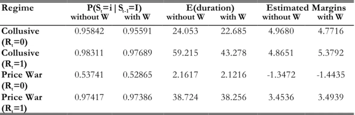
(18) Table 3 Diagnostic Tests Test for9 Serial Correlation – Collusion Regime Serial Correlation – Price War Regime ARCH Higher-order Markov Dependence – Collusion Regime Higher-order Markov Dependence – Price War Regime Joint Test. Without Wholesale Price Statistic p-value 0.42 0.517. With Wholesale Price Statistic p-value 0.03 0.868. 0.31. 0.575. 0.00. 0.982. 0.55 10.93. 0.460 0.000. 0.49 16.99. 0.485 0.000. 0.061. 0.813. 0.07. 0.797. 16.49. 0.006. 25.73. 0.000. As the results in table 3 above, the joint test finds strong evidence of misspecification in both of the specifications we report. However, this evidence appears to be entirely confined to evidence of higher-order Markov dependence in the collusive regime; the test statistics are more than ten time larger than those for any other single test, and their pvalues are the only ones below 20%.. The Effects of Regulation on Price Wars In both specifications and in both sets of equations (margin and regime selection) considered, the parameters associated with the regulation dummy (Rt) are positive and significant only during price wars. This result is consistent with the theoretical model where a price floor regulation has no effect on prices (or margins) during collusive periods since the monopoly price is assumed to be charged during those periods. However, our results show that during price war regimes, the price floor regulation increases both margins and probabilities of continuing the price war. Table 4 reports estimated regime dependent conditional probabilities (using equation 7), durations (using. 9. Each individual test statistic has an asymptotic ? 2(1) distribution under the null hypothesis of no misspecification, while the joint test is asymptotically distributed as a ?2(5) under the null.. 15.

(19) 1/(1 − q), where q is the regime dependent conditional probability) and margins (using equations 10 and 11), all computed from the estimates presented in Table 2.. Table 4 Regime Dependent Statistics Regime Collusive (Rt =0) Collusive (Rt =1) Price War (Rt =0) Price War (Rt =1). P(St =i|St-1=I). E(duration). Estimated Margins. without W. with W. without W. with W. without W. with W. 0.95842. 0.95591. 24.053. 22.685. 4.9680. 4.7716. 0.98311. 0.97689. 59.215. 43.278. 4.8651. 5.3792. 0.53741. 0.52865. 2.1617. 2.1216. -1.3472. -1.4435. 0.97417. 0.97386. 38.724. 38.256. 3.4536. 3.4939. During collusive regimes, the transition probabilities are similar before and after regulation and their estimates are robust to the inclusion/exclusion of the wholesale. However, during price war regimes, transition probabilities are significantly higher after regulation (increasing from around 0.53 to 0.97) again, regardless of the specification considered.. Regulation also increased the expected duration of both regimes, with the effect more pronounced during price wars. Before regulation, price wars lasted two weeks on average, while after regulation they last an average of 38. For comparison, collusive regimes lasted about 24 weeks before regulation versus 43 to 59 weeks after, depending on the specification used.. Results on estimated margins are fully consistent with the theory. On one hand, during collusive regimes, estimated margins are about the same magnitudes with and without a price floor regulation. On the other hand, regulation increases significantly the margins during price wars: from approximately –1.5 cents to 3.5 cents with a price floor. However, regulation did not raise price war margins to the level of collusive margins.. 16.

(20) Under regulation, price war and collusive regimes both seem to last longer but margins are significantly larger during price wars than they were without price regulation. The total effect on average margin (and therefore average price) of the price floor is therefore still ambiguous. It may be the case that the effect of the increase in margins during price wars and the effect of the increase of the duration of collusive regimes are not fully compensated by the higher prevalence of price wars under regulation.. Table 5 presents estimated unconditional probabilities of the collusive regime (this is 1 – the corresponding probability for the price war regime) as well as the unconditional expected margin. From those figures, it appears that the increase in margins during price wars has been almost exactly offset by the increase in the average duration of a price war, resulting in no significant change in the average margins in the industry. In other words, the price floor regulation had little or no effect on average margins (and therefore prices) even if margins are now higher during price wars, simply because those wars now last longer.. Table 5 Unconditional Probabilities and Margins State. Rt =0 Rt =1. P(St =collusive) without W with W. 0.91753 0.60461. 0.91447 0.53079. Estimated Margins without W with W. 4.4472 4.3070. 4.2400 4.4946. Sample Margins. 4.4205 4.4158. 5. Concluding Remarks. The application of Abreu’s optimal punishment model to a Bertrand oligopoly supergame predicts that, when products are highly substitutable and sellers are many (which is the case in the studied market), the duration of punishment should be shorter without regulation than when a price floor applies. This theoretical prediction is entirely supported by our empirical findings. The results obtained with a Markov Switching Model using data on the Montreal retail market for gasoline show that the introduction of. 17.

(21) a price floor regulation reduces the intensity of price wars but raises their expected duration.. Two important implications arise from our empirical results. First, since the introduction of a price floor has little or no effect on prices or margins, regulation provided no longterm “protection” for marginal (inefficient) firms in the form of higher prices. Because regulation reduced the intensity of price wars, the potential for large financial losses during a short period of time is reduced. However, firms are now more frequently in price wars. The net impact on the competitiveness of the retail gasoline industry is therefore ambiguous, but apparently small.. Second, given the robust support the data give to our theoretical predictions, it appears that the retail market for gasoline in Montreal is accurately described by a model without coordination or explicit collusion between firms. Absent such anti-competitive behaviour, and given the first implication above, the price-floor regulation in this market seems useless.. 18.

(22) References Abreu, Dilip J. (1986), “Extremal Equilibria of Oligopolistic Supergames”, Journal of Economic Theory 39(1), 191-225. Borenstein, Severin (1991), “Selling Costs and Switching Costs: Explaining Retail Gasoline Margins”, RAND Journal of Economics 22(3), 354-369. Borenstein, Severin and Andrea Shepard (1996), “Dynamic Pricing in Retail Gasoline Markets”, RAND Journal of Economics 27(3), 429-451. Filardo, Andrew J. (1994) “Business-Cycle Phases and Their Transitional Dynamics” Journal of Business and Economic Statistics, vol. 12, issue 3, pages 299-308. Filardo, Andrew J. and Stephen Gordon (1998) "Business Cycle Durations", Journal of Econometrics, 85 (1), 99-123. Häckner, Jonas (2000), “A Note on Price and Quantity Competition in Differentiated Oligopolies”, Journal of Economic Theory 93(2), 233-239. Hamilton, James D. (1993), “Estimation, Inference and Forecasting of Time Series Subject to Changes in Regime”. In G. S . Maddala, C. R. Rao, and H. D. Vinod, eds., Handbook of Statistics, Vol. 11, North-Holla nd. Hamilton, James D. (1994),“Time Series Analysis”, Princeton University Press, 799 p. Hamilton, James D. (1996), “Specification Testing in Markov-Switching Time-series Models”, Journal of Econometrics 70(1), 127-157. Kim, Chang-Jin and Charles R. Nelson (2001), “State-Space Models with Regime Switching: Classical and Gibbs-Sampling Approaches with Applications”, MIT Press, 1999, 297 p. Lambertini, Luca and Dan Sasaki (2002), “Non-negative Quantity Constraints and the Duration of Punishment”, Japanese Economic Review 53(1), 77-93. Lee, Lung-Fei and Robert H. Porter (1984), “Switching Regression Models With Imperfect Sample Separation Information – With An Application on Cartel Stability”, Econometrica 52(2), 391-418. Porter, Robert H. (1983), “A Study of Cartel Stability: the Joint Executive Committee, 1880-1886”, The Bell Journal of Economics 14(2), 301-314. Slade, Margaret E. (1992), “Vancouver’s Gasoline-Price Wars: An Empirical Exercise in Uncovering Supergame Strategies”, Review of Economic Studies 59(2), 257-276.. 19.

(23) Appendix. A.1 Without regulation In this section, we compute the optimal punishment price p L and the threshold level. δ (γ ) of the discount factor, for all values of γ over the range (0,1) , in the absence of regulation. For this purpose, recall that the demand for product i in each period is. qi ( p) =.  (1 + γ (n − 2)) γ (n − 1)  1  1 − pi + p j , 1 + γ (n − 1)  1 −γ 1−γ . (A.1). all i. As π i = pi qi , it follows that one-shot symmetric individual profits when all firms charge the same price p ∈ {p L , p H } are. − π ( p ) = (1 p ) p . γ (n − 1) + 1. (A.2). Negative outputs do not make economic sense. It is easy to check that q i ≥ 0 if and only if. pi ≤. 1 − γ + γ (n − 1) p j , 1 + γ (n − 2). (A.3). all i, j ∈ N , i ≠ j . These n inequalities define the set of prices for which all nonnegativity constraints in quantities are satisfied, that is a cone with apex pˆ = (1,K ,1) , as illustrated by point A in Figure A.1 (for n = 2 ).. 20.

(24) Figure A.1. (n=2) The dashed lines, which intersect at point A, represent the. q i = 0 constraints, i = 1,2 (see expressions (A.3) with a strict equality sign). The thick segments describe firm i’s best reply function Ri ( p j ) , for all p j ∈ [−c, p H ], i, j = 1,2, i ≠ j. The shaded area describes firms’ prices for which non-negativity constraints are satisfied (i.e., q i ≥ 0 ) and the regulation price is not binding (i.e., p i ≥ p R ≡ 0 ).. pj. 1. −. pH. −. γ 2 +γ −2 γ2 −2. −. pi =. 1−γ γ + pj 2 2. pi =. p i = 1 + γ (1 + p j ). −. C. γ −1 1 + pj γ γ − A. Ri ( p j ). − c≥ −1 0. γ −1 γ. −. −B. γ 2 −1 γ2 −2. 1. pi. − − −c ≥ − 1. 21.

(25) For a given price p j as charged by all n − 1 firms j in N, with j ≠ i, the specific form of firm i’s best reply function Ri ( p j ) , and consequently of the one-shot deviation profit function π id ( p j ) , depend on the status of constraints (A.3).10 There are four possible cases: a) either no constraint is binding, or b) firm i’s constraint is not binding and all other firms’ constraints are binding, or c) firm i’s constraint is binding and all other firms’ constraints are not binding, or d) all firms’ constraints are binding. The latter case is trivial, as no firm produces. We examine the former three cases in turn, as follows:. a) if no constraint is binding, firm i’s best reply function is obtained by the first-order condition for a maximum in π i ( pi , p j ) , all p j , to give. Ri ( p j ) =. 1 − γ + γ (n − 1) p j , 2(1 + γ ( n − 2 )). (A.4). and. π id ( p j ) =. (1 − γ + γ ( n − 1) p j ) 2 1 ; 4 (1 − γ )(1 + γ (n − 1)) + (1 + γ ( n − 2 )). (A.5). b) if firm i’s constraint only is not binding, the best reply in p i to all p j is obtained by setting each other firm’s output expression equal to zero, to find. Ri ( p j ) =. γ − 1 + (1 + γ (n − 2)) p j γ (n − 1). ,. (A.6). and. π id ( p j ) =. 1 [1 + γ (2 n − 3)][1 − γ − (1 + γ ( n − 2 )) p j ]( p j − 1) ; 4 γ 2 (n − 1) 2 (1 + γ (n − 1)). (A.7). 10. In this appendix, we index best reply functions and one-shot optimal deviation functions by subscripts i, j ∈ N , i ≠ j . In the main body of the paper, these subscripts were omitted whenever possible, for simplicity in the notation.. 22.

(26) c) if firm i’s constraint only is binding, the best reply in p i to all p j is simply. Ri ( p j ) = 0,. (A.8). π id ( p j ) = 0,. (A.9). and then. where i, j ∈ N , i ≠ j . We can now determinate which of the latter three particular forms of π id ( p j ) in (A.5), (A.7), or (A.9), as plugged in the system of simultaneous equations (1 – 2), leads to a solution ( p L , δ (γ )) for a given value of the differentiation parameter γ in (0,1). To see that, note that firm i’s best reply function Ri ( p j ) , as obtained in the no binding constraint case a), intersects firm i’s expression of non-negativity frontier (A.3) at point.  γ −1  ) )  < (0,0) , ( pi , p j ) =  0,  γ (n − 1)  (A.10) all i, j ∈ N , i ≠ j (see point B in Fig. A.1), and also intersects firm j’s expression of nonnegativity frontier (A.3) at point.   ( ( (γ ( 2 n − 3) + 1)(1 − γ ) (γ (3n − 5) + 2)(1 − γ ) ( pi , p j ) =  2 2 ,  (0 ,0) ,  γ ( n − 6 n + 7 ) + 2( 2γ ( n − 2) + 1) γ 2 ( n 2 − 6 n + 7 ) + 2 (2γ ( n − 2) + 1)  >  . (A.11). all i, j ∈ N , i ≠ j (see point C in Fig. A.1). Then consider firm i’s one-shot optimal deviation from p j = p H ≡ 1 / 2 . From the strict inequality in (A.10), we know that the best-reply and deviation profit functions in case c) cannot apply, as they are defined only if p j < 0 (which is strictly less than p H ). And the strict inequality in (A.11) implies that we must look for the border between cases a) and. 23.

(27) b). This is done by looking for the differentiation parameter values for which the two ( cases coincide, that is by solving the equation p j = p H for γ , all n ≥ 2 . This yields. γ′=. 1+ 3 . n+ 3. (A.12). For γ < γ ′ case a) applies, otherwise case b) applies. Now consider firm i’s one-shot optimal deviation from p j = p L < 1 / 2 . The best-reply and deviation profit functions in case b) do not lead to an admissible solution ( p L ,δ (γ )) . As p L is an endogenous variable, we need first to compute it before obtaining the border between cases a) and c), as follows. •. Assume first that case a) applies for firm i’s optimal one-shot deviation from both. p L and p H . In this case we find a solution ( p L ,δ (γ )) , which is displayed in Table # for the case n = 2 only, for clarity. 11 It is easy to check that ) ) p L ∈ ( p j , p H ) , with p j as in (A.7), and that δ (γ ) ∈ (0,1) , for all γ < γ ′ , with γ ′ as in (A.12), and for all n ≥ 2 . •. Then assume that cases a) and b) apply for firm i’s optimal one-shot deviation from p L and p H , respectively. Again we find a solution ( pL′ , δ ′(γ )) , and here ) ( ) ( also it is easy to check that p ′L ∈ [ p j , p j ) , with p j and p j as in (A.10), and that. δ ′(γ ) ∈ (0,1) , for all n ≥ 2 and only if γ ≤ γ ′′ , with. γ ′′ =. 3 5 +5 , 2n + 3( 5 + 1). (A.13). and for all n ≥ 2 .. Expressions of optimal punishment prices are displayed for all n ≥ 2 in the next section of the appendix. Since we do not use the (space consuming) algebraic expressions of the corresponding threshold levels for the discount factor, we do not display them in this paper. They are available from the authors upon request. 11. 24.

(28) •. Eventually, assume that cases c) and b) apply for firm i’s optimal one-shot deviation from p L and p H , respectively. We find a third solution ( p ′L′ ,δ ′′(γ )) , ) ) and here again it is easy to check that p ′L′ ∈ (−1, p j ] , with p j as in (A.7), and that. δ ′ (γ ) ∈ (0,1) , for all γ ≥ γ ′′ , with γ ′′ as in (A.13), and for all n ≥ 2 .. We check that the individual rationality condition in the punishment phase is satisfied. This is done by verifying that ∞. π ( p L ) + ∑ [δ (γ )]τ π ( p M ) ≥ 0,. (A.14). τ =1. for p L = p L , p ′L , p ′L′ and δ (γ ) = δ (γ ),δ ′(γ ),δ ′′(γ ) , respectively, as obtained above. The left-hand side term of the latter inequality is the sum of two terms. The first one is the individual profit obtained when all firms charge p L in a period of a punishment. The second term is the value of individual discounted profits when all firms charge the collusive price p H after the punishment period onwards. When (A.14) does not hold, all firms find it preferable not to sell, as the losses incurred in the punishment period overbalance the discounted stream of collusive profits.. A.2 With regulation The three optimal punishment prices, as obtained in the previous section in the absence of regulation, are. 1 2 − γ (n + 1) , pL = 2 2 + γ ( n − 3). (A.15). for γ ∈ (0, γ ′) , and. 25.

(29) p ′L =. γ (n − 1)(1 − γ ) − (1 − γ )[γ (n − 2) + 1][γ 2 (n 2 − n − 1) − (n − 3)γ − 1] , γ (n − 1)[2 + γ (n − 3)]. (A.16). for γ ∈ [γ ′, γ ′ ) , and. p ′L′ =. 1 γ (n − 1) − [γ (nγ − 1)(2n − 3) + 1] , γ (n − 1) 2. (A.17). for γ ∈ [γ ′′,1) , all n ≥ 2 .. Simple comparisons lead to the ranking. p L ≥ p ′L ≥ p ′L′ .. (A.18). Now by using (A.15), we find. p L > p R ≡ 0 if and only if γ <. 2 ≡ γ1, n +1. (A.19). all n ≥ 2 . By considering (A.18) and (A.19) together, we conclude that, when the products are sufficiently close substitutes, in the sense that γ ≥ γ 1 , we obtain. p R ≥ p L ≥ p ′L ≥ p ′L′ . In that case, the regulation price is binding. Then by comparing γ 1 with γ ′ and γ ′′ , as displayed in (A.12) and (A.13) respectively, we check that. γ 1 < γ ′ < γ ′′ .. (A.20). 26.

(30) Table A.1. (n=2) Optimal punishment price p L and threshold level for all values of γ in (0,γ ′) , [γ ′, γ ′′) , and [γ ′′,1) .. γ. pL. δ (γ ). 2 − 3γ 2 (2 − γ ). (2 − γ ) 2 16(1 − γ ).  3 5 − 5   3 − 1, 2  . γ (1 − γ ) − (1 − γ )(γ 2 + γ − 1) (2 − γ )γ. (2 − γ ) 2 (γ 2 + γ − 1). 3 5 −5     2 ,1  . γ − (1 + γ )(2γ − 1) 2γ. (0,. ). 3 −1. (γ. 2. + 2 (1 − γ )(γ 2 + γ − 1). ). 2. γ 2 + γ −1 2 2γ + γ − 1. 27.

(31)