The Perils of Confounding Factors: How Fitts' Law Experiments can Lead to False Conclusions

HAL Id: hal-01690122

https://hal.archives-ouvertes.fr/hal-01690122

Submitted on 22 Jan 2018

HAL is a multi-disciplinary open access

archive for the deposit and dissemination of

sci-entific research documents, whether they are

pub-lished or not. The documents may come from

teaching and research institutions in France or

abroad, or from public or private research centers.

L’archive ouverte pluridisciplinaire HAL, est

destinée au dépôt et à la diffusion de documents

scientifiques de niveau recherche, publiés ou non,

émanant des établissements d’enseignement et de

recherche français ou étrangers, des laboratoires

publics ou privés.

The Perils of Confounding Factors: How Fitts’ Law

Experiments can Lead to False Conclusions

Julien Gori, Olivier Rioul, Yves Guiard, Michel Beaudouin-Lafon

To cite this version:

Julien Gori, Olivier Rioul, Yves Guiard, Michel Beaudouin-Lafon. The Perils of Confounding Factors:

How Fitts’ Law Experiments can Lead to False Conclusions. CHI’ 18, Apr 2018, Montréal, Canada.

�10.1145/3173574.3173770�. �hal-01690122�

The Perils of Confounding Factors: How Fitts’ Law

Experiments can Lead to False Conclusions

Julien Gori

_{Olivier Rioul}

_{Yves Guiard}

_{Michel Beaudouin-Lafon}

1

_{LTCI, Telecom ParisTech}

Université Paris-Saclay

F-75013, Paris, France

2

_{LRI, Univ. Paris-Sud, CNRS,}

Inria, Université Paris-Saclay

F-91400, Orsay, France

{

}

ABSTRACT

The design of Fitts’ historical reciprocal tapping experiment gravely confounds index of difficulty ID with target distance D: Summary statistics for the candidate Fitts model and a com-peting model may appear identical, and the validity of Fitts’ model for some tasks can be legitimately questioned. We show that the contamination of ID by either target distance D or width W is due to the common practices of pooling and averaging data belonging to different distance-width (D,W) pairs for the same ID, and taking a geometric progression for values of D and W. We analyze a case study of the validation of Fitts’ law in eye-gaze movements, where an unfortunate experimental design has misled researchers into believing that eye-gaze movements are not ballistic. We then provide simple guidelines to prevent confounds: Practitioners should carefully design the experimental conditions of (D,W), fully distinguish data acquired for different conditions, and put less emphasis on r2 _{scores. We also recommend investigating the use of}

stochastic sampling for D and W. ACM Classification Keywords

H.5.2. Information Interfaces and Presentation (e.g. HCI): User Interfaces

Author Keywords

Fitts’ law; factor confounds; models INTRODUCTION

Fitts’ law is a well known rule for human-aimed movement that predicts the movement time (MT) it takes to reach a target of width W located at a distance D:

MT = a + b log₂(1 + D/W) = a + b ID, (1) where ID is the index of difficulty1and a and b are estimated empirically.

This is the author’s version. It is posted here by permission of ACM. Not for redistribution. All rights retained by ACM. The definitive version will be publishedCHI 2018, April 21-26, Montreal, Canadahttps: //doi.org/10.1145/3173574.3173770

Fitts’ law gained importance in the HCI community after the seminal study by Card et al. [4] that measured the performance of four pointing devices on desktop computers. The law plays a prominent role in HCI, where it is heavily used to predict and evaluate the performance of input techniques. It has been shown to handle many conditions and tasks quite well, result-ing in an incredibly wide spectrum of applications. Studies include reciprocal tapping between two targets using different limbs and body parts, such as tapping pedals [9] and manipu-lating a cursor [15] with the feet, controlling a stylus attached to the chin with head movements [2], and moving a cursor by rolling the head [16]. More unexpected applications include pointing and dragging sequences [12], rapid elbow flexion [6], eye-gaze movements [25, 21], and a study of patients with cerebral palsy [3],

Fitts’ pointing paradigm for the reciprocal tapping experi-ment [10, Experiexperi-ment I] has proven to be very influential. Fitts’ apparatus was comprised of two plates of width W, separated by distance D. Distance and width were systemati-cally varied: The four different conditions of D (2,4,8,16 (in.)) were crossed with four conditions for W (1/4,1/2,1,2 (in.)), resulting in 16 conditions. MT was then evaluated for each one of the 16 conditions. Today’s version of a generic 1-D Fitts’ law experiment is in many cases a simple adaptation of this protocol, where physical plates are replaced by targets on computer screens, and reciprocal tapping is sometimes re-placed by discrete tapping, a cleaner version of the protocol due to Fitts & Peterson [11]. While the ISO standard [24] for the evaluation of pointing performance recommends a 2-D multi-directional tapping task, composed of circular targets of diameter W arranged in a circle of diameter D to control the effect of direction, many studies, old or recent, are conducted with the simple 1-D task.

Notations

Throughout the paper we use the following notations: ● Factorsare noted in roman capital letters: distance D, width

W, index of difficulty ID, and movement time MT.

1

There are several formulations for ID, the one given here, known as the Shannon formulation [18, 19] being the most widely used in HCI.

● These factors take values in sets, denoted by their corre-sponding calligraphic capital letters: D = {d1, d2, . . . , dn},

W = {w1, w2, . . . , wm}, ID = {id1, id2, . . . , idk}.

● When two factors, e.g. D and W, are fully crossed, each element of D is paired with each element of W, resulting in n × m pairs. We use the condensed notation D × W to denote all these pairs.

● Several (D,W) pairs may result in the same D/W ratio. For example if D = {10, 20, 50} and W = {1, 2, 4}, pairs (10,1) and (20,2) have the same D/W ratio of 10. We call D the variable corresponding to the average distance computed over equal ratiosD/W.

● The list of averaged values D is noted D. With D and W as above, the set of ratios is {2.5, 5, 10, 12.5, 20, 25, 50} and the corresponding list of values of D is D = (10, 15, 15, 50, 20, 50, 50).

● Similarly, we note MT and W the variables corresponding to the averages of MT and W computed over equal ratios D/W.

Flaws in Fitts’ Literature

While Fitts’ law has proven to be incredibly robust and useful, a number of potential flaws in the experimental designs used in the literature have been identified.

Guiard [14] showed that the design of Fitts’ original tapping experiment correlates ID with D: “ The dependence [between D and ID] is strong and systematic: on average target distance is raised by 11.7 cm for each extra bit of information” [14]. Hence Fitts’ design makes D a confounding factor: a factor that has an effect on both a dependent and an independent variable in a controlled experiment.

It may then appear that manipulating the independent variable leads to variations in the dependent variable, when in fact both variations are due to the confounding factor. Thus, within Fitts’ design, manipulating the ID affects movement time, but in fact both ID and MT are affected by the confounding factor D, making it impossible to disentangle the effects of D and ID on MT.

The correlations between D and ID are even stronger if one “builds an average on execution times for one ID first and

calcu-late the correlation afterwards” [7]. This procedure, commonly used by HCI researchers, considers all blocks corresponding to the same ID as equivalent and computes a single average per value ofID, leading to what we have noted D, W and MT. Not only does this operation pre-supposes the validity of Fitts’ law [7, 8], it also strongly correlates D and ID [14, 7, 8]. As we shall illustrate, it then becomes impossible do distinguish if the effects on MT are due to D or ID.

The implications of these confounds are wide ranging. Accord-ing to MacKenzie [20], referrAccord-ing to Glencross and Barrett [13], “It has been suggested that the model [Fitts’ law] would hold for the mouth or any other organ for which the necessary de-grees of freedom exist and for which a suitable motor task could be devised”. If D is indeed a confounding factor for ID, one can then wonder about the validity of Fitts’ law in some of its applications.

Positioning and Goals of The Paper

One solution proposed by Guiard [14] to disentangle D and ID is what he called the complete form x scale design. Although this solution does guarantee the decorrelation of D and ID, it is impractical for pointing experiments in that it strongly restrains the range of variation of ID2_{. The ID cannot be}

raised over 6 bits or so because that would require, at lower scale levels, impractically small values of W; nor can the ID be lowered below 4 bits or so because that would require, at higher scale levels, impractically large values of D [14]. While the form×scale design ensures a totally independent variation of factors D and ID, in “real-world” HCI, the deci-sion about the validity of Fitts’ law is usually based on the informal criterion that r2between ID and MT should be high enough (e.g., r2

> 0.9 in [24]). What matters then, as we will show, is not that the confound be totally removed, but rather that its “strength” be reduced. We define X and Y as strongly confoundedfactors if r2(X, Y) > 0.9, otherwise they are weakly confounded3. In contrast to Guiard [14], the focus of this paper is to find designs that prevent strong confounds. The goal of this paper is threefold: First, we identify the ob-jective conditions that lead to strong confounds in Fitts’ law experimental designs. Such conditions can be evaluated on past and future experiments to quickly determine if the design is at risk of strong confounds. Second, once these conditions are clearly identified, we show a documented case in eye-gaze pointing where the validation of Fitts’ model is the result of a strong confound between D and ID. Third, we provide rec-ommendations to protect the experimenter from confounding factors when designing experiments for Fitts’ law. These rec-ommendations may also prove useful for experimenters in HCI in general.

PRACTICAL EFFECTS OF STRONG CONFOUNDS Guiard [14] and Drewes [7, 8] have illustrated the strong confound between D and ID that occurs in Fitts’ original design and raised ensuing qualitative issues. The goal of this section is to show a numerically worked out example of strong confounds between D and ID, on a different design than Fitts’. A Surprising Simulation

Let us consider two potential generative processes for MT: Law A is Fitts’ law, where MT is given by Eq. (1). Values

for a and b are taken respectively as a = −1047 ms and b =391 ms/bit.

Law B relates MT to D only: MT = a′

+b′D, (2) where a′_{= −251 ms and b = 1.956 ms}/mm.

The explanation for the specific values of a, a′_{, b and b}′_will

appear below. We now consider the following experimental

2

As noted in [14], a full form×scale design on Fitts’ design for Experiment I [10] requires, e.g., W = 0.02 cm.

3_{The operational value of r}2 _{above which a confound is deemed} strong or not depends of course on what is expected by the experi-menter. The value .9 is common in the Fitts’ law literature.

3.17 4.08 5.04 6.02 7.01

Index of Difficulty

Mo

vemen

t

Time

(ms)

Figure 1. Simulated data for task A (orange, logarithmic) and task B (blue, linear). We have shifted the x-axis by 0.05 for task A for better legibility. The circles correspond to the average MT for a given ID for task B, the diamonds for task A. For Fitts’ law (task A), we find MT= 386 ID− 1040 with r2= 0.9995. For task B, we find MT = 392 ID − 1052 with r2_{= 0.9921.}

design: D = {256, 512, 1024} and W = {8, 16, 32}, where D and W are fully crossed. There are thus 9 different exper-imental conditions that lead to only 5 different D/W ratios: (8,16,32,64,128). The corresponding average distances are D = (256,384,597,768,1024).

We run a simulation experiment where trials for each process are generated for the D × W conditions by adding a random noise sample to the underlying generative process. MTifor

each trial i is then given by,

MTi= −1047 + 391 log2(1 + D/W) + zi (law A) (3)

MTi= −251 + 1.956 D + z ′

i, (law B) (4)

where ziand z′iare the outcomes of a centered random process,

which we took equally distributed according to a zero-mean Gaussian law with standard deviation σ = 300 ms, meaning that approximately 96% of the samples for MT are located within a 1200 ms interval. As we shall see later, the shape of the actual distribution is of little impact as long as it is centered.

We generated 200 trials per condition; the two datasets are represented in a MT vs. ID plane in Fig. 1. Five vertical scatters are obtained, one for each different D/W ratio. To get rid of the strong variability, we consider MT, the averages of MT per ID. After averaging, we end up with the blue dots and orange diamond markers in Fig. 1.

The surprising result is that the summary MT for law A is indistinguishable from that of law B. Both datasets, after aver-aging, are extremely well fitted with Fitts’ law: The r-squared between MT and ID is r2

=0.9995 for law A and r2=0.9921 for law B. This is unexpected for the second dataset since it was generated with law B, not Fitts’ law.

A Scenario for an Experimenter

The scenario for the above simulation is very close to a real experiment: Let us consider an experimenter who wants to investigate two tasks A and B and tries to find reasonable models to explain MT in both tasks. Let us assume that MT is actually governed by law A (Fitts’ law) for task A and by law B for task B. The experimenter does not know this but has the intuitionthat both tasks should be reasonably well modeled by Fitts’ law (law A).

After setting up the experimental design described above, he runs the experiment for both tasks. The resulting datasets are probably very similar to those in Fig. 1, with 5 vertical scatters for each task. After averaging over ID, he ends up with the large markers (blue disks and orange diamonds) of Fig. 1. This is precisely the averaging procedure discussed by Drewes [7] and mentioned in the introduction. After averaging, the experimenter then computes a fit using linear regression, and finds very high r2’s for both tasks. He can thus conclude that his intuition was right and that Fitts’ law is a good model to describe MT for both tasks. Unfortunately, as we have shown, in the case of task B, this is an artifact due to the experimental design.

Decoding the Simulation

We now explain the results of the simulation.

Law A

For a given ID, the average of MT is equal to Fitts’ law evalu-ated at this given ID, plus the average value of the zi’s. Since

the noise is centered, the law of large numbers implies that the average value of the noise is close to 0. While we used a Gaussian distribution, this holds for any shape of the noise distribution. We could also have used an asymmetric distri-bution to guarantee positive movement times, this would not have changed the values obtained after averaging. A similar observation can be made about the standard deviation. By virtue of the central limit theorem, a larger standard deviation would only require more trials for the sample mean to be close enough to the statistical mean.

Thus, the fact that we get an r2_{between MT and ID close to}

1 for law A is not surprising. As expected, we find that the linear regression between MT and ID is very close to the one used for generating the data: MT = 386 ID − 1040 for the simulation results vs. MT = 391 ID − 1047 for the formula generating the data.

Law B

The dataset generated with law B has the same summary statis-tic as the one generated with law A. Although surprising, this can be explained as follows. In the MT versus ID plane, there can be more than one (D, W) condition leading to the same D/W ratio, e.g. for D/W = 32, there are three different values for D: D = 1024 (W = 32), D = 512 (W = 16), and D = 256 (W = 8). Therefore while it appears that there is only one verti-cal scatter plot per ID, there are in fact three overlapping ones. As the contribution of the noise will again be close to zero by the law of large numbers, average MT can thus be evaluated by inputting the average D = 1/3 × (256 + 512 + 1024) ≃ 600 into

3.17 4.08 5.04 6.02 7.01

ID

D

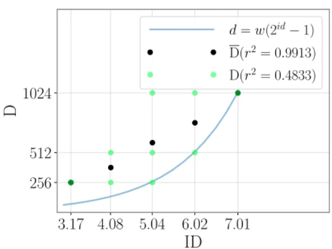
Figure 2. The 9 D conditions (light green dots) that lead to the 5 ID conditions used in the thought experiment. Black dots correspond to D, the average value of D for equal IDs. Dark green dots correspond to data points that overlap the average. r2_{between D and ID and between D and}

ID are given in the legend. The blue line corresponds to Eq. 8.

Eq. 2. By generalizing over all values of ID, MT is obtained simply by evaluating Eq. 2 for each value of D.

Fig. 2 plots the values of D appearing in the D × W conditions (light green dots) and those appearing in D (black dots) against ID. The correlation between D and ID is very high (r2 = 0.9913). This means that the relationship between D and ID can be considered linear:

D = α + β ID, (5) Linear regression gives α = −407 and β = 200. Inputting Eq. (5) into Eq. (2), we find that MT is given by

MT = a′

+b′D = a′+b′α + b′β ID = a′′+b′′ID, (6) thereby showing that MT will indeed appear linear in ID. Notice that this situation can only happen if the confound between ID by D is strong enough, which warrants our focus on strong confounds.

The values used in the simulation can now be explained: We chose the values of a and b and computed a′ _{and b}′ _from

Eq. (6). We can verify that a = a′_+b′α = −251+1.956×−407 =

−1047 and b = b′β = 1.956 × 200 = 391.

Strong Confounds in the Goal Passing Task

The previous simulation is not entirely artificial. In fact, the D × Wconditions, as well as the values4of a and b are from Accot & Zhai’s goal passing task [1, Experiment 1]. They conducted this experiment to validate Fitts’ law as a model for

4

Accot & Zhai [1] actually give a = −1347 instead of the −1047 that we used. We did so because the values of the fit given in their paper do not match the plot in their figure. For example, for ID = 3.5, we can read MT ≃ 300 ms in the graph, but a calculation using the values of the fit predicts 21.5 ms. We assume that there was a typographical error, whereby the “0” in 1047 was mistakenly typed as a “3”.

goal passing, a result that they used in the derivation of the steering law.

Accot & Zhai used 9 conditions, yet only represented 5 move-ment time averages [1, Fig. 3], each corresponding to a di ffer-ent ID, meaning that they considered MT. According to the simulation above, we now know that another law than Fitts’ law, whose formula is given by Eq. (2), will fit MT equally well. Note that since one law depends on W and not the other, one of the two models must prove inaccurate in a design that does not confound D and ID so strongly.

Accot & Zhai were apparently unaware of this difficulty, and concluded that the “goal passing task follows the same law as in Fitts’ tapping task despite the different nature of movement constraint”. They used the word “despite” as if surprised that Fitts’ law proved a good predictor for movement times. In fact, the law given by Eq. (2) seems reasonable for a goal passing task when W is large enough, since in that case the width does not really constrain the movement and the goal passing task becomes a simple distance covering task. As-suming a constant maximum speed c, movement time would simply be given by

MT = to+1/c × (D − d0), (7)

where t0is the time needed to reach a speed of c, and d0the

distance traveled until c is reached. This is a linear model as in Eq. (2) with slope 1/c and intercept t0−d0/c.

CONDITIONS FOR STRONG CONFOUNDS

Fitts’ design for the tapping experiment [10, Experiment I] strongly confounds D with ID (r2 between D and ID above .99, see [14, 8]). We have established that the design of the goal passing task [1, Experiment 1] suffers from a similar confound (r2between D and ID above .99). In this section, we investigate the reason for these strong confounds.

Fitts-Like Designs

We first define a class of experimental designs, which we call Fitts-like designs, characterized by experimental conditions of the following general form:

1. D = {d.2i}, where 0 ≤ i ≤ N − 1 and d is fixed, 2. W = {w.2j_{}, where 0 ≤ j ≤ M − 1 and w is fixed.}

3. D and W are fully crossed.

Conditions 1 and 2 state that the values of D and W follow a geometric progression. Both Accot & Zhai’s goal passing task and Fitts’ tapping experiment are Fitts-like designs.

Table 1 shows the r2values between D and ID for four Fitts-like designs: “Tapping”, “Disc Transfer” and “Pin Transfer” refer to the experiments conducted by Fitts [10]; “Goal Pass-ing” refers to the study conducted by Accot & Zhai [1, Ex-periment 1]. All four exEx-periments lead to strong confounds between D and ID.

We also compute the r2_{values between D and ID for different}

sizes of D and W. Fig. 3 shows that any Fitts-like design strongly confounds D with ID if N and M are small enough. Practical considerations often limit the values of N and M to

XP N/M d w r2(D, ID) r2(W, ID) Tapping 4/4 2(in.) 1/4(in.) 0.99 0.94

Disc Transfer 4/4 4(in.) 1/16(in.) 0.97 0.97 Pin Transfer 5/4 1(in.) 1/16(in.) 0.95 0.94 Goal Passing 3/3 256(pix.) 8(pix.) 0.99 0.99

Table 1. Characteristics of four Fitts-like experiments. Tapping, Disc Transfer and Pin Transfer by Fitts (1954) and Goal Passing by Ac-cot& Zhai (1997).

about 5, so that most Fitts-like designs are likely to produce strong confounds between D and ID.

Geometric Progression of D&W Causes Strong Confound The strong confound between D and ID is the result of the geometric progressions of D and W. First, notice that D is an exponential function of ID (Fig. 2):

d = w × (2id−1) (8) For D to be strongly confounded with ID, i.e. to be linearly de-pendent of ID, D must combine several values corresponding to the same ID. If a design is fully crossed, there are at least two values of ID corresponding to a single (D, W) condition, namely the minimum ID (minimum D associated with maxi-mum W) and the maximaxi-mum ID (maximaxi-mum D associated with minimum W). In the case of Fitts-like designs, only these two IDs meet this condition, as can be seen in Fig. 2.

Let us now construct a design where there are multiple values of D for each ID, except for the extreme ones. We start with a predetermined set ID = {id1, id2, . . . } of increasing IDs.

We can then always choose the values of D and compute the corresponding W using the definition of ID. Assuming that the design is fully crossed, the smallest ID, id1, is necessarily

composed by the smallest D (d1) and the largest W (w1). We

pick an arbitrary value for d1and solve id1=log₂(1 + d1/w1) for w1, giving

w1=d1/(2id1−1)

Since we do not allow a single D condition for a given value of ID (except at the edges), the second smallest value of ID, id2, should correspond to the two combinations d1×w2and

d2×w1, from which the values of w2and d2can be computed:

id2=log₂(1 + d1/w2) Ô⇒ w2=d1/(2id2−1) id2=log₂(1 + d2/w1) Ô⇒ d2=w1× (2id2−1) Note that we have d2/d1=w1/w2.

The next smallest value of ID, id3, must correspond to at

least two of the following combinations: (d3, w1), (d1, w3),

(d2/w2), i.e. d3/w1 = d2/w2 and d1/w3 = d2/w2. Solving

these gives d3 =d2w1/w2 and w3 =w2d1/d2. Note that we

have d3/d2=w1/w2=d2/d1and w3/w2=d1/d2=w2/w1. 2 3 4 5 6 7 8 9 10 11 12 13 14 Number of D conditions 2 3 4 5 6 7 8 9 10 11 12 13 14 Num b er of W conditions

r2_{values between D and ID}

0.5 0.6 0.7 0.8 0.9

Figure 3. r2_{values between D and ID when N (number of D conditions)}

and M (number of W conditions) are varied. White dots indicate the cases where r2≥ 0.95. r2computed for d= 128 and w = 12 according to our notation of Fitts-like designs.

We repeat this procedure for the remaining values of ID. It follows that the increasing sequence of distances diand the

de-creasing sequence of widths wjare such that all ratios di/di+1

and wj+1/wjare equal, except at the edges, resulting in

geo-metric progressions for the values of D and W.

The fact that the resulting values of D are almost in linear progression can be explained mathematically, but is of little interest: it is a coincidence due to the fact that the range of IDs being investigated is small. This explains why r2decreases when N and M increase, as shown in Fig. 3.

To summarize, the fact that Fitts-like designs create strong confounds between D and ID can be attributed to the following causes:

1. D and W are both in geometric progressions (one passes from one value to the next by multiplying by some constant, e.g. 2);

2. the range of IDs used in practice is small.

Other Strong Confounds

We have just identified the reasons that make Fitts-like designs strongly confound D with ID. As W grows at the same rate as D, one would expect an equivalently strong confound in Fitts-like designs between W and ID. This is indeed the case as can be seen in the rightmost column of Table 1. One should thus also be careful to avoid strong confounds between W and ID.

Care must also be taken with designs that are not Fitts-like. The combination of a small number of conditions, the fact that they are usually chosen according to some structure (such as a linear or geometric progression), and the smoothing effect of averaging make it very likely that D or W can be approached by a simple function of ID.

We illustrate this with an example. Consider a candidate model5for the dependent variable Y as a function of the inde-pendent variable X:

Y = f (X). (9) Now consider a third variable Z, that can be expressed as a function of X:

Z = g(X). (10) We will call g the confusion function. A competing model of the form

Y = f (g−1(Z)) (11) will inevitably be indistinguishable from the candidate model, since plugging (10) into (11) gives:

Y = f (g−1(g(X))) = f (X) (12) which is equivalent to Eq. (9).

The variable Z used here is very general and can represent any factor. In the example developed in the previous section (“Thought experiment”), ZwasD and the g was a linear func-tion. As another, more complex example, let us consider two sets D and W for which D has a square root relationship to ID D = a′√_{ID + b}′ ₍₁₃₎

Then, g−1(x) = (x/a′

)2−b′, and f (g−1(x)) = a − bb′+ b(x/a′

)2, so that a quadratic model for MT cannot be dis-tinguished from Fitts’ model, as MT is also linearly related to ID. If we then take a model of the form

MT = a − bb′

+b(D/a′)2 (14) plugging Eq. (13) into Eq. (14) gives

MT = a + bID. (15) This is a simple linear function between MT and ID, thereby showing that a quadratic law for movement time can be indis-tinguishable from Fitts’ law in some designs.

While in general, a weak confound between D and ID implies that any function of D is (weakly) confounded with ID, this is not true anymore for strong confounds. We have shown here that most designs of Fitts’ law experiments are likely to have a strong confound between ID and some function of D and W. If one knows precisely this strong confound, e.g. Eq. (13), it is easy to determine which model for MT will have almost the same summary statistic MT and r2as Fitts’ model. For example, with Eq. (13), consider the model of Eq. (14). Creating Strong Confounds Between Any Two Factors In the previous subsections, we explained how strong con-founds between ID and functions of D or W could make two models indistinguishable from each other. We now give a general method to create strong confounds between ID and almost any function of D or W, as a constructive illustration.

5

In Fitts’ law, Y ≡ MT, X ≡ ID, and f is a linear function. X, Y and Zmay also represent averaged quantities, e.g. D or MT.

1. Choose a set of ID values ID, 2. Choose a set of target sizes W.

3. Choose the confusion function, e.g. D = 4.5√ID − 0.9. 4. For each target size w ∈ W and for each id ∈ ID , find the

corresponding Dw,id= (2id−1)w.

5. For each ID, find the combination of D’s whose average minimizes the distance to the target confusion function.

Figure 4. A generic method that generates a design to create confound-ing variables

Fig. 4 shows a method for creating (D,W) pairs that strongly correlate ID with any function of D. Confounding with W is easily achieved by switching the roles of D and W. Extra search steps could be added to the algorithm. For example, in step 2, one could consider several sets W and keep the one that minimizes the distance to the target confusion function; in step 3, the parameters of the confusion function could be varied.

We used the procedure described in Fig. 4 with the following confusion function from Eq. (13):

D = 4.5 √

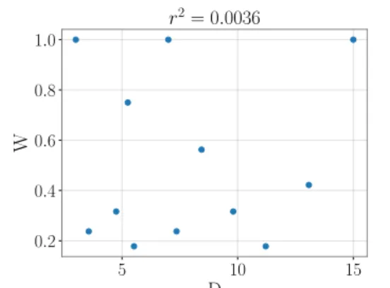
ID − 0.9. (16) The corresponding D and W conditions, resulting in 12 pairs, are given in Fig. 5. Notice that in resulting design D and W are almost as well decorrelated as in a fully crossed design. We then perform the same simulation as in the Thought Ex-periment: Law A is given by Fitts’ law, as before, and Law B is the quadratic law in Eq. (14). After the simulation of 200 trials per condition, we find that r2_{between MT and ID}

is once again very high for Law A: r2=0.99. It is also very high for Law B: r2=0.95. As in the Thought Experiment, the summary statistics of the two laws are almost identical. More importantly, we obtain very good fits for movement time using Fitts’ law in a situation where the data for movement time was generated using a quadratic law that does not depend on the width factor W. 5 10 15 D 0.2 0.4 0.6 0.8 1.0 W r2_{= 0.0036}

Figure 5. D and W conditions that lead to an almost perfect confusion between D and√ID. The correlation between W and D is r2_{= 0.0036.}

In summary, we first demonstrated that Fitts-like designs cre-ate strong confounds between D and ID. We then showed that the issue is much deeper than Fitts-Like designs: With any design, there exists a possibility that some function of D or W is strongly confounded with ID.

EYE-GAZE EXPERIMENTS

We discuss two studies conducted on eye-gaze movements us-ing the results of the previous section. These demonstrate that the issues we have underlined until now are not only theoreti-cal constructs, but do appear in real-world scenarios. The first study, by Miniotas [21], validated Fitts’ model for movement time in a pointing task using eye-gaze. Drewes [8] discussed this study and pointed out that outside HCI, researchers would generally use Carpenter’s formula [5] (a formula not dependent on W) to model eye-gaze data. We compare this first study to another study by Miniotas et al. [22], as yet uncommented, and show that the results of these two studies on the validity of Fitts’ model for eye-gaze data are strikingly inconsistent. We will explain the difference by formally applying Carpenter’s formula to Miniotas’ paradigm and using the previous results on Fitts-like designs.

Fitts’ Law for Eye-Gaze Interaction

The first study [21] was conducted to validate Fitts’ law for modeling eye-gaze interactions. According to Miniotas [21], prior work by Ware and Mikelian [25] suggested that Fitts’ law would be an adequate model for movement time in eye-gaze interaction, but the range of ID explored then was very narrow (less than 3 bit wide), and the width W had been kept constant. The motivation was thus to create an empirical dataset that was more thorough.

In line with Fitts’ paradigm, the task was to move the cur-sor to a target of width W located at a distance D by us-ing their eyes instead of a stylus. An eye tracker was used to control the cursor. The control variables were D (D = {26, 52, 104, 208} (mm)) and W (W = {13, 26} (mm)). It is not clear how the r2_{between MT and ID was computed,}

but Miniotas reported r2=0.982. He concluded that Fitts’ law was a good fit for his dataset, a valuable result for designers. However, it turns out that the design of the experiment is “Fitts-like” according to our definition: First, both D and W have a geometric progression; there are 8 conditions, yet only 5 different D/W ratios. Second, the range of IDs, [1, 4.1], is quite small. Accordingly, the correlation between D and ID is very strong: r2 =0.974, leading to a strong confound. As a consequence, a competing model such as Eq. (2) could equally well explain the summary of the gathered data. Note that Ware & Mikelian [25], recognizing that eye-saccades are ballistic, stated that they had used Fitts’ law “only as a con-venient way of summarizing the results, not because [they] wish[ed] to make any theoretical claims”.

Carpenter’s Formula

A reliable relation known as Carpenter’s formula [5] relates MT and angular amplitude α (Eq. (17)) for eye-gaze move-ments:

MT = a + b α, (17)

L

S α

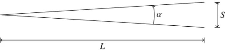
Figure 6. Carpenter’s Formula applied to Fitts’ pointing paradigm. L is the fixed distance between the user and the screen, S is the on-screen distance that the cursor must travel, i.e. D with the notations of Eq. (1).

where MT is the movement time needed to cover the angular amplitude α. Carpenter’s formula can be applied to Miniotas’ paradigm as illustrated in Fig.6, where L is fixed and S corre-sponds to D in Fitts’ paradigm. In line with the ballistic nature of eye movements, W does not appear in Carpenter’s formula. The angle α can be expressed in terms of the available param-eters as α = 2 arctan (S 2L) ≃ S L = D

L when α is small enough. (18) If we input this equation into formula Eq. (17), we obtain

MT = a + b α ≃ a + b′

D, where b′

=b/L. (19) Therefore, Carpenter’s formula, the leading explanatory model, predicts that movement time is linearly related to D.

Thanks to our previous analysis, we can now safely assert that since the design of Miniotas’ experiment [21] is Fitts’ like, Fitts’ model is almost equivalent in terms of fitting MT to the leading explanatory model derived from Carpenter’s formula. Therefore one cannot conclude from that experiment that eye-gaze follows Fitts’ law.

Eye-Gaze Interaction with Expanding Targets

Miniotas et al. [22] conducted a second study on eye-gaze interaction with expanding static targets. Expanding static targets are targets whose appearance does not change for the user, but to which the interface responds as if it were larger. The expansion is predetermined, hence the term “static”. Although the goal was not to validate Fitts’ law, Miniotas et al. did check for goodness of fit of the Fitts model and found r2=0.69. The experiment is very similar to that described in the first study [21], with a notable exception: the progression for W is not geometric, but linear: D = {128, 256, 512} (pix.) and W = {12, 24, 36} (pix.). Because this design is not Fitts-like, we expect r2between D and ID to be weaker than for Fitts-like designs, and indeed we find r2

=0.74.

Miniotas et al. attributed the decrease in correlation between MT and ID from 0.98 in the 2000 study [21] to 0.69 in the 2004 study [22] to the presence of a visible cursor in the 2000 study,

XP Fitts-like r2(D, id) r2(MT, id) Miniotas 2000 yes 0.99 0.98 Miniotas et al. 2004 no 0.74 0.69

Table 2. Table summarizing the relevant r2_{in the Miniotas (2000) and}

Miniotas et al. (2004) studies. r2_{(x, y) is the coefficient of determination}

whereas there was no visual feedback in the 2004 study. This is because they assumed Fitts’ law to be a valid model. However, the comparison between the two studies tells a different story, as shown in Table 2. The design used in the 2000 study [21] was Fitts-like, making Fitts’ model almost equivalent to the one derived from Carpenter’s formula, whereas the design used in the 2004 study [22] was not Fitts-like. As a result the confound between D and ID is not as strong (r2 between D and ID of .74). Not surprisingly, r2between MT and ID drops with a similar magnitude (r2_{between MT and ID of .69). We}

conclude that Fitts’ model’s apparent validity in [21] is an artifact caused by the experimental conditions.

COMBATING STRONG CONFOUNDS

In this section we give four recommendations to protect exper-iment designers from strong confounds.

Do Not Trust a Goodr2

The two datasets generated from law A and law B in the Thought Experiment had the same MT and r2. From this sum-mary alone, they were indistinguishable. If one had used dif-ferent summaries, such as those from Jude et al. [17], striking differences would have emerged. For example, the variance of the two datasets are very different.

The evaluation of Fitts’ model in the HCI community relies almost exclusively on high r2 values. As emphasized by Roberts & Pashler [23] however, a good fit reveals nothing about the flexibility and variability of the data (what the model can and cannot fit), nor the likelihood of other models. Indeed, we have shown that within a Fitts-like design, two different models could fit the same summary data.

Do Not Average or Pool Data From Different Conditions We have seen (Sect. 3) that the strong confound between D and ID was made possible because of the averaging procedure. For example, in Fitts’ tapping experiment, the r2between D and ID is .48; after averaging the r2between D and ID is .99. It is unfortunately common for experimenters to pool data and average movement times that correspond to the same D/W ratio but that do not come from the same D ×W condition (see, e.g., Drewes [7, 8]). This practice involves a confirmation bias: The logic behind averaging movement times that correspond to the same D/W ratio but come from different pairs (D,W) is to believe that because data was acquired under the same ratio and that movement time is supposedly dependent on the ratio only, the two conditions would essentially be the same. But this is only true if indeed, the ratio explains all the variability of MT, which is precisely what we want to test when trying to validate Fitts’ law in the first place.

Averaging before knowing the validity of Fitts’ model may then result in a premonitory experiment where Fitts’ law can be validated simply because it was pre-supposed to hold, as shown in the section analyzing Miniotas’ experiment [21]. Note that for experimenters using the effective index of dif-ficulty, IDe [24], a different value of IDe is calculated for

each block based on the participants variability in that specific block. Therefore different conditions will almost always result

in different values of IDe, even if they correspond to the same

D/W ratio. The net result is that this procedure eliminates the risk of averaging across (D, W) conditions.

Consider Competing Models

We have shown that Fitts-like designs create strong confounds between ID and both D and W. We further showed that we could construct a design that strongly confounds ID with al-most any simple function of D or W. It is then important, when evaluating whether Fitts’ model is a good fit for a task, to also consider competing models. If there are any, the experimenter should make sure that the design does not strongly confound factors of both models. For example, in the eye-gaze study it would have been safer to also evaluate Carpenter’s formula (Eq. 17) on the experimental data.

Notice that once a competing model is identified, it is easy to verify the risk of strong confounds among factors by checking the correlations between them.

Use Stochastic Conditions

In a Fitts’ law experiment, D and W are varied and MT is measured. The average MT of each block represents one sample in the (D,W) space. Experimental data can thus be visualized as a set of samples in the (D,W) space6. Fitts [10] showed that this representation could be summarized by a simple formula – now known as Fitts’ law. We have shown that some sampling strategies such as Fitts’, i.e. geometric progressions and orthogonal sampling in the (D,W) space, may lead to strong confounds between factors. A different sampling strategy is Guiard’s [14] orthogonal sampling in the form×scale space, which provides a theoretical solution to the issue, but can lead to physical values of D and W that are hard to implement in practice.

We have shown that sampling issues leading to strong con-founds occur under very specific conditions, i.e. when the conditions are generated by some rule. For example, a Fitts-like design is characterized by a geometric progression for D and W. Therefore, we believe that a simple solution to get rid of potential sampling artifacts is to adopt stochastic conditions for D and W, possibly with some constraints. For example, we could divide the (D,W) space into a grid and choose ex-perimental conditions by drawing a point uniformly within each rectangle defined by the grid, resulting in pairs of (D,W) values).

CONCLUSION AND PERSPECTIVES

In the experimental testing of any mathematical model, we may distinguish two steps:

1. Sampling the factor space, e.g. Fitts’ traditional (D, W) space or Guiard’s form×scale space, thus defining a set of experimental conditions for data collection;

2. Processing the data by applying operations that yield a score. In Fitts’ law studies, this traditionally involves computing means of movement times and r2 values between ID and MT.

6

Incidentally, this is precisely how Fitts summarized his data in his historical study [10, Fig. 4]

We have shown that a Fitts-like sampling of the (D, W) space solely associated with the computation of r2between ID and MT creates strong confounds between D and ID. We attributed this to the geometric progression of D and W. A simple workaround would seem to be to avoid such a sampling. How-ever, using a constructive approach, we devised a sampling strategy that strongly confounds ID with any simple function of D and W. Avoiding Fitts-like designs is thus insufficient to avoid strong confounds.

Based on these new results, we analyzed an apparent contradic-tion between the results of two eye-gaze pointing experiments using. We resolved the contradiction by noting that Carpen-ter’s formula is a widely accepted model for eye-gaze data and by showing that in one of the experiments, Fitts’ model was indistinguishable from Carpenter’s model due to the use of a Fitts-like design.

Finally, we provide guidelines to avoid strong confounds be-tween factors. We believe that Fitts’ law studies place too much emphasis on high r2values. It is crucial to introduce other considerations when validating a model, such as the flexibility of the evaluated model, the variability of the dataset and the possibility of competing models. Working with block averages or, worse, averages computed for equal values of ID, such as MT, dramatically decreases the number of points to be fitted, thereby mechanically increasing r2values.

An interesting and simple way to prevent strong confounds is to use stochastic sampling of the (D,W) space. Stochastic sampling is a promising perspective, especially when consid-ering the replication of studies, as a different but equivalent design can be ensured with each replication. However, more conceptual work is needed to support the idea of using random conditions in a controlled experiment.

ACKNOWLEDGMENTS

This research was partially funded by Labex DigiCosme (ANR-11-LABEX-0045-DIGICOSME), operated by the French Agence Nationale de la Recherche (ANR) as part of the program “Investissement d’Avenir” Idex Paris-Saclay (ANR-11-IDEX-0003-02), and by ERC European Research Council (ERC) grant 695464 “ONE: Unified Principles of Interaction”. REFERENCES

1. Johnny Accot and Shumin Zhai. 1997. Beyond Fitts’ law: models for trajectory-based HCI tasks. In Proceedings of the ACM SIGCHI Conference on Human factors in computing systems. ACM, ACM, New York, NY, USA, 295–302. DOI:http://dx.doi.org/10.1145/258549.258760

2. Robert O Andres and Kenny J Hartung. 1989. Prediction of head movement time using Fitts’ law. Human Factors 31, 6 (1989), 703–714.

3. Pedro E. Bravo, Miriam LeGare, Albert M. Cook, and Susan Hussey. 1993. A Study of the Application of Fitts’ Law to Selected Cerebral Palsied Adults. Perceptual and Motor Skills77, 3_suppl (1993), 1107–1117. DOI:

http://dx.doi.org/10.2466/pms.1993.77.3f.1107

4. S. K. Card, W. K. English, and B. J. Burr. 1978. Evaluation of mouse, rate-controlled isometric joystick,

step keys, and text keys for text selection on a CRT. Ergonomics21, 8 (1978), 601–613. DOI:

http://dx.doi.org/10.1080/00140137808931762

5. Roger HS Carpenter. 1988. Movements of the Eyes, 2nd Rev. Pion Limited, London.

6. Daniel M. Corcos, Gerald L. Gottlieb, and Gyan C. Agarwal. 1988. Accuracy Constraints Upon Rapid Elbow Movements. Journal of Motor Behavior 20, 3 (1988), 255–272. DOI:

http://dx.doi.org/10.1080/00222895.1988.10735445

PMID: 15078623.

7. H. Drewes. 2010. Only One Fitts’ Law Formula Please!. In CHI ’10 Extended Abstracts on Human Factors in Computing Systems (CHI EA ’10). ACM, New York, NY, USA, 2813–2822. DOI:

http://dx.doi.org/10.1145/1753846.1753867

8. H. Drewes. 2013. A Lecture on Fitts’ law. (2013).

http://www.cip.ifi.lmu.de/~drewes/science/fitts/ ALectureonFittsLaw.pdf

9. Colin G. Drury. 1975. Application of Fitts’ Law to Foot-Pedal Design. Human Factors 17, 4 (1975), 368–373. DOI:

http://dx.doi.org/10.1177/001872087501700408

10. P. M. Fitts. 1954. The information capacity of the human motor system in controlling the amplitude of movement. Journal of experimental psychology47, 6 (1954), 381. DOI:http://dx.doi.org/10.1037/h0045689

11. Paul M Fitts and James R Peterson. 1964. Information capacity of discrete motor responses. Journal of experimental psychology67, 2 (1964), 103. DOI:

http://dx.doi.org/10.1037/h0045689

12. Douglas J Gillan, Kritina Holden, Susan Adam, Marianne Rudisill, and Laura Magee. 1990. How does Fitts’ law fit pointing and dragging?. In Proceedings of the SIGCHI conference on Human factors in computing systems. ACM, ACM, New York, NY, USA, 227–234. DOI:

http://dx.doi.org/10.1145/97243.97278

13. D. J. Glencross and N. Barrett. 1989. Discrete movements. In Human skills (D. H. Holding (Ed.)). John Wiley, Oxford, England. 107–146 pages.

14. Yves Guiard. 2009. The problem of consistency in the design of Fitts’ law experiments: Consider either target distance and width or movement form and scale. In Proceedings of the SIGCHI Conference on Human Factors in Computing Systems. ACM, ACM, New York, NY, USA, 1809–1818. DOI:

http://dx.doi.org/10.1145/1518701.1518980

15. Daniel Horodniczy and Jeremy R. Cooperstock. 2017. Free the Hands! Enhanced Target Selection via a Variable-Friction Shoe. In Proceedings of the 2017 CHI Conference on Human Factors in Computing Systems (CHI ’17). ACM, New York, NY, USA, 255–259. DOI:

16. Thibaut Jacob, Gilles Bailly, Eric Lecolinet, Géry Casiez, and Marc Teyssier. 2016. Desktop Orbital Camera Motions Using Rotational Head Movements. In Proceedings of the 2016 Symposium on Spatial User Interaction (SUI ’16). ACM, New York, NY, USA, 139–148. DOI:

http://dx.doi.org/10.1145/2983310.2985758

17. Alvin Jude, Darren Guinness, and G Michael Poor. 2016. Reporting and Visualizing Fitts’s Law: Dataset, Tools and Methodologies. In Proceedings of the 2016 CHI

Conference Extended Abstracts on Human Factors in Computing Systems. ACM, ACM, New York, NY, USA, 2519–2525. DOI:

http://dx.doi.org/10.1145/2851581.2892364

18. I. S. MacKenzie. 1989. A note on the

information-theoretic basis for Fitts’ law. Journal of motor behavior21, 3 (1989), 323–330. DOI:

http://dx.doi.org/10.1080/00222895.1989.10735486

19. I. S. Mackenzie. 1992. Fitts’ law as a performance model in human-computer interaction. Ph.D. Dissertation. University of Toronto.

20. I Scott MacKenzie. 1992. Fitts’ law as a research and design tool in human-computer interaction.

Human-computer interaction7, 1 (1992), 91–139. DOI:

http://dx.doi.org/10.1207/s15327051hci0701_3

21. Darius Miniotas. 2000. Application of Fitts’ Law to Eye Gaze Interaction. In CHI ’00 Extended Abstracts on

Human Factors in Computing Systems (CHI EA ’00). ACM, New York, NY, USA, 339–340. DOI:

http://dx.doi.org/10.1145/633292.633496

22. Darius Miniotas, Oleg Špakov, and I. Scott MacKenzie. 2004. Eye Gaze Interaction with Expanding Targets. In CHI ’04 Extended Abstracts on Human Factors in Computing Systems (CHI EA ’04). ACM, New York, NY, USA, 1255–1258. DOI:

http://dx.doi.org/10.1145/985921.986037

23. Seth Roberts and Harold Pashler. 2000. How persuasive is a good fit? A comment on theory testing.

Psychological review107, 2 (2000), 358. DOI:

http://dx.doi.org/10.1037/0033-295X.107.2.358

24. R William Soukoreff and I Scott MacKenzie. 2004. Towards a standard for pointing device evaluation, perspectives on 27 years of Fitts’ law research in HCI. International journal of human-computer studies61, 6 (2004), 751–789. DOI:

http://dx.doi.org/10.1016/j.ijhcs.2004.09.001

25. Colin Ware and Harutune H. Mikaelian. 1987. An Evaluation of an Eye Tracker As a Device for Computer Input. In Proceedings of the SIGCHI/GI Conference on Human Factors in Computing Systems and Graphics Interface (CHI ’87). ACM, New York, NY, USA, 183–188. DOI:http://dx.doi.org/10.1145/29933.275627