Preconditioned Krylov subspace methods for solving radiative transfer problems with scattering and reflection

This section considers the development of finite element subspaces satisfying the crucial inf-sup condition in Assumption 3.1.. Lemma 4.1 below provides several equivalent

A significant result derived in this paper is the superlinear convergence of the GMRES algorithm when it is preconditioned with the so called Schwarz preconditioner in the case of

In order to check the validity of the present dual method, we compare the stress fields obtained using this method with the stress fields obtained using the classical displacement

Schwarz preconditioning combined with GMRES, Newton basis and deflation DGMRES: preconditioning deflation AGMRES: augmented subspace. 11

Freund, Reduced-order modeling of large linear subcircuits via a block Lanczos algorithm, in: Proceedings of the 32nd ACM=IEEE Design Automation Conference, ACM, New York, 1995,

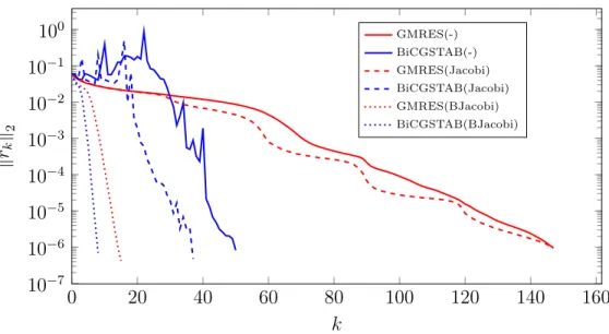
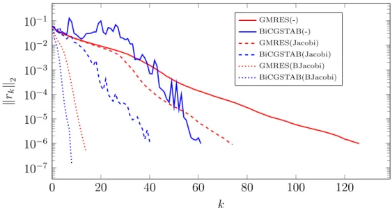
3, it is shown how the number of iterations evolves with the number of degrees of freedom (dof) for the four implemented solving methods: three solvers (COCG, BiCGCR, QMR) with

Krylov Subspace Methods for Inverse Problems with Application to Image Restoration.. Mohamed

In Section 4, we define EGA-exp method by using the matrix exponential approximation by extended global Krylov subspaces and quadrature method for computing numerical solution

References

[1] M. F. Modest, Radiative heat transfer, Academic press, 2013.
[2] G. Krishnamoorthy, R. Rawat, P. J. Smith, Parallelization of the p1
radiation model, Numerical Heat Transfer, Part B: Fundamentals 49 (2006) 1–17.
[3] L. Ruan, W. An, H. Tan, H. Qi, Least-squares finite-element method of multidimensional radiative heat transfer in absorbing and scattering media, Numerical Heat Transfer, Part A: Applications 51 (2007) 657– 677.
[4] Y. Lu, A. F. Chatziioannou, A parallel adaptive finite element method for the simulation of photon migration with the radiative-transfer-based model, Communications in numerical methods in engineering 25 (2009) 751–770.
[5] D. Balsara, Fast and accurate discrete ordinates methods for multidi-mensional radiative transfer. Part I, basic methods, Journal of Quanti-tative Spectroscopy and Radiative Transfer 69 (2001) 671–707.
[6] D. Le Hardy, Y. Favennec, B. Rousseau, Solution of the 2-D steady-state radiative transfer equation in participating media with specular reflections using SUPG and DG finite elements, Journal of Quantitative Spectroscopy and Radiative Transfer 179 (2016) 149–164.
[7] W. Fiveland, Discrete-ordinates solutions of the radiative transport equation for rectangular enclosures, Journal of Heat Transfer 106 (1984) 699–706.
[8] D. Boffi, F. Brezzi, M. Fortin, Mixed finite element methods and ap-plications, volume 44 of springer series in computational mathematics, 2013.
[9] D. Le Hardy, M. A. Badri, B. Rousseau, S. Chupin, D. Rochais, Y. Favennec, 3D numerical modelling of the propagation of radiative in-tensity through a X-ray tomographied ligament, Journal of Quantitative Spectroscopy and Radiative Transfer 194 (2017) 86–97.
(26)
[10] O. Lehtikangas, T. Tarvainen, A. Kim, S. R. Arridge, Finite element approximation of the radiative transport equation in a medium with piecewise constant refractive index, Journal of Computational Physics 282 (2015) 345–359.
[11] D. Le Hardy, Y. Favennec, B. Rousseau, F. Hecht, Specular reflection treatment for the 3D radiative transfer equation solved with the discrete ordinates method, Journal of Computational Physics 334 (2017) 541– 572.
[12] W. An, L. Ruan, H. Qi, L. Liu, Finite element method for radiative heat transfer in absorbing and anisotropic scattering media, Journal of Quantitative Spectroscopy and Radiative Transfer 96 (2005) 409–422. [13] M. Badri, P. Jolivet, B. Rousseau, S. Le Corre, H. Digonnet, Y.
Faven-nec, Vectorial finite elements for solving the radiative transfer equation, Journal of Quantitative Spectroscopy and Radiative Transfer 212 (2018) 59–74.
[14] M. A. Badri, P. Jolivet, B. Rousseau, Y. Favennec, High perfor-mance computation of radiative transfer equation using the finite el-ement method, Journal of Computational Physics (2018).
[15] D. Mihalas, Stellar atmospheres, San Francisco, WH Freeman and Co., 1978. 650 p. (1978).
[16] M. L. Adams, E. W. Larsen, Fast iterative methods for discrete-ordinates particle transport calculations, Progress in nuclear energy 40 (2002) 3–159.
[17] E. W. Larsen, Transport acceleration methods as two-level multigrid algorithms, Operator Theory: Advances and Applications 51 (1991) p34–47.
[18] I. C. Ipsen, C. D. Meyer, The idea behind Krylov methods, American Mathematical Monthly (1998) 889–899.
[19] S. Turek, A generalized mean intensity approach for the numerical so-lution of the radiative transfer equation, Computing 54 (1995) 27–38.
(27)
[20] M. Seaıd, M. Frank, A. Klar, R. Pinnau, G. Th¨ommes, Efficient numer-ical methods for radiation in gas turbines, Journal of Computational and Applied Mathematics 170 (2004) 217–239.
[21] B. W. Patton, J. P. Holloway, Application of preconditioned GMRES to the numerical solution of the neutron transport equation, Annals of Nuclear Energy 29 (2002) 109–136.
[22] W. F. Godoy, P. E. DesJardin, On the use of flux limiters in the discrete ordinates method for 3D radiation calculations in absorbing and scat-tering media, Journal of Computational Physics 229 (2010) 3189–3213. [23] S. Balay, S. Abhyankar, M. F. Adams, J. Brown, P. Brune, K. Buschel-man, L. Dalcin, V. Eijkhout, W. D. Gropp, D. Kaushik, M. G. Knepley, L. C. McInnes, K. Rupp, B. F. Smith, S. Zampini, H. Zhang, H. Zhang, PETSc web page, 2017.
[24] M. A. Heroux, R. A. Bartlett, V. E. Howle, R. J. Hoekstra, J. J. Hu, T. G. Kolda, R. B. Lehoucq, K. R. Long, R. P. Pawlowski, E. T. Phipps, et al., An overview of the Trilinos project, ACM Transactions on Math-ematical Software (TOMS) 31 (2005) 397–423.
[25] H. A. Van der Vorst, Bi-CGSTAB: A fast and smoothly converging variant of Bi-CG for the solution of nonsymmetric linear systems, SIAM Journal on scientific and Statistical Computing 13 (1992) 631–644. [26] Y. Saad, M. H. Schultz, GMRES: A generalized minimal residual
al-gorithm for solving nonsymmetric linear systems, SIAM Journal on scientific and Statistical Computing 7 (1986) 856–869.
[27] W. E. Arnoldi, The principle of minimized iterations in the solution of the matrix eigenvalue problem, Quarterly of applied mathematics 9 (1951) 17–29.
[28] M. Avila, R. Codina, J. Principe, Spatial approximation of the radi-ation transport equradi-ation using a subgrid-scale finite element method, Computer Methods in Applied Mechanics and Engineering 200 (2011) 425–438.
[29] W. H. Reed, New difference schemes for the neutron transport equation, Nuclear Science and Engineering 46 (1971) 309–314.
(28)
[30] Y. Saad, Iterative methods for sparse linear systems, SIAM, 2003. [31] L. G. Henyey, J. L. Greenstein, Diffuse radiation in the galaxy, The
Astrophysical Journal 93 (1941) 70–83.
[32] F. Robert, E. Alain, Berlingot, http://www.mathcurve.com/ surfaces/berlingot/berlingot.shtml, 2017.
[33] O. Axelsson, Iterative solution methods, Cambridge university press, 1996.
[34] G. Kanschat, Solution of radiative transfer problems with finite ele-ments, in: Numerical methods in multidimensional radiative transfer, Springer, 2009, pp. 49–98.
[35] S. Turek, An efficient solution technique for the radiative transfer equa-tion, Impact of computing in science and engineering 5 (1993) 201–214.
Figure
Figure 1: Discretized angular space with the icosahedron refinements. (a) icosahedron, (b) first refinement icosahedron, and (c) second refinement icosahedron.
Figure 2: Dirichlet boundary conditions and the geometry used for the tests in section 4.