Université de Montréal
i’Iining Dynarnic Databases for Freqttent Closed Iterusets
par Jtin Jing
Département d’informatique et de recherche opérationnelle faculté tics arts et tics sciences
Mémoire présenté à la Faculté des Études Supérieures en vue de l’obtention du grade de
maîtrise ès sciences M.Sc. en Informatique
Juillet 2004
o
p
r ‘ot]5
2DQ
Direction des bibliothèques
AVIS
L’auteur a autorisé l’Université de Montréal à reproduire et diffuser, en totalité ou en partie, par quelque moyen que ce soit et sur quelque support que ce soit, et exclusivement à des fins non lucratives d’enseignement et de recherche, des copies de ce mémoire ou de cette thèse.
L’auteur et les coauteurs le cas échéant conservent la propriété du droit d’auteur et des droits moraux qui protègent ce document. Ni la thèse ou le mémoire, ni des extraits substantiels de ce document, ne doivent être imprimés ou autrement reproduits sans l’autorisation de l’auteur.
Afin de se conformer à la Loi canadienne sur la protection des renseignements personnels, quelques formulaires secondaires, coordonnées ou signatures intégrées au texte ont pu être enlevés de ce document. Bien que cela ait pu affecter la pagination, il n’y a aucun contenu manquant. NOTICE
The author of this thesis or dissertation has gtanted a nonexclusive license allowing Université de Montréal to reproduce and publish the document, in part or in whole, and in any format, solely for noncommercial educational and research purposes.
The author and co-authors if applicable retain copyright ownership and moral rights in this document. Neither the whole thesis or dissertation, nor substantial extracts from it, may be printed or otherwise reproduced without the author’s permission.
In compliance with the Canadian Privacy Act some supporting forms, contact information or signatures may have been removed from the document. While this may affect the document page count, it does not represent any loss of content from the document.
Université de Montréal Faculté des Études Supérieures
Ce mémoire intitulé
Mining Dynarnic Databases for Frequent C!eed Itemsets
présenté par: Jun Jing
a été évalué par un jury composé des personnes suivantes
Gefia Hahn Président Rapporteur Petko Valtchev Directeur de recherche Mikiés CsLrôs Membre du Jury
Résumé
La fouille de données, aussi connue sous le nom de la découverte de connaissance dans la base de données (DDBC), consiste à découvrir des informations cachées et utiles dans des grandes bases de données. La découverte des règles d’association est une branché importante de la fouille de données. Elle est utilisée pour identifier des dépendances entre articles dans une base de données. L’extraction des règles d’association a été prouvée pour être très utile dans le commerce et les champs d’activité qui lui sont proche.
La plupart des algorithmes d’extraction des règles d’association appliquent à des bases de données statiques seulement. Si la base de données se développe (nouvelles transactions sont ajoutées), nous devrions re-exécuter ces algorithmes du début pour toutes les transactions afin de produire le nouvel ensemble des règles d’association parce que l’ajout de nouvelles transactions peut rendre des itemsets fréquents (itemsets fréquents fermés) invalide ou
générer de nouveaux itemsets fréquents (itemsets fréquents fermés), ce qui influence les règles d’association. Ces algorithmes n’essayant pas d’exploiter les résultats obtenus de l’ensemble des transactions.
À
ce jour, plusieurs algorithmes incrémentaux de mise à jour progressive ont été développés pour la maintenance des règles d’association.Dans cette thèse, nous traitons les aspects algorithmiques de l’extraction des règles d’association. Particulièrement, nous nous concentrons surl’analyse de quelques algorithmes incrémentaux basés sur les connexions de Galois, comme GALIC’IA et GALI(’IA-T. Nous avons aussi étudié certains algorithmes de calcul d’iternsets fréquents, comme Apriori
algorithm. En se basant sur ces algorithmes, nous proposons un nouvel algorithme, appelé l’algorithme de treillis d’iceberg (ILA), qui utilise peu d’opérations pour maintenir à jour la
structure de l’iceberg lors de l’insertion d’une nouvelle transaction dans l’ensemble des transactions. Ceci devrait être utile pour l’amélioration de la performance des algorithmes existants basés sur le treillis de Galois (le treillis de concept).
Mots clés: treillis de Galois (concept), treillis iceberg, algorithme de construction de treillis, méthodes incrémentales.
Mining Dynamic Databases for Frequent Closed Itemsets Il
Abstract
Data Mining, also known as Knowledge Discovery in Databases (KDD), is the discovery of hidden and meaningftil information in a ‘arge database. Association rule mining is an important branch of data mining. It is used to identify relationships within a set of items in a database (or transaction set). Association mie mining has been proven to be very useful in
the retail communities, marketing and other more diverse fields.
Most association rule mining algorithms apply to static transaction sets only. If the transaction set evolves (i.e. new transactions are added), one needs to execute these algorithms from the beginningto generate the new set ofassociation rules, since aciding new transactions may invalidate existing frequent itemsets (or frequent closed itemsets) or generate new ftequent itemsets (or frequent closed itemsets), which wiIl influence the association rules. These algorithms do not attempt to exploit the resuits obtained from the original transaction sets. To date, many incrementai updating proposais have been developed
to maintain the association rules.
In this thesis, we deal with the algorithmic aspects of association rLlIe mining. Specifically, we focus on analyzing some incremental algorithms based on Galois connection, such as GALIcL4, and GALICJA-T. We also study some plain frequent itemsets mining algorithms, sctch as Apriori algorithm. Based on these, we propose a new algorithm, called Iceberg
Lattice Algorithm (ILA), which uses oniy a few operations to maintain the iceberg structure
when a new transaction is added to transaction set. It should be helpful in improving the performance of existing algorithms that are based on Gaiois lattices (concept lattices). Key words: Galois (concept) iattices, iceberg lattices, lattice constructing algorithms,
Contents
Résumé jAbstract
II
List of tables
V
List of figures
vi
Acknowledgments
VIIIChapter I Introduction
11.1 What is DataMining? 1
1 .2 Association rule mining 2
1.3 Ourcontribution 3
1.4 Thesis organization 3
Chapter II
Data
Mining 42. 1 Association rule mining 4
2.1 .1 Basic concepts of association ru les 5
2.1 .2 Basics of concept lattices 6
2.2 Current state ofresearch onassociation rute miningalgorithms 13
2.2.1 Plain frequent itemsets mining algorithms 13
2.2.2 Frequent closed itemsets mining algorithrns 14
2.2.3 Incrernental FI or FCI mining algorithrns 15
2.3 Review oftwo typical algorithms 16
2.3.1 Apriori algorithm 16
2.3.2A-Close algorithm
18
Chapter III Review of the GALICIA approach 22
3.1 Lattice updates 22
Mining Dynamic Databases for frequent Closed Itemsets IV
3.2.1 GALICIAscheme 27
3.2.2 GALICJA-T 28
Chapter IV Maintain iceberg lattices only with FCTs 32
4. IncrernentaÏ iceberg lattices update 32
4.2 Theoretical deveïopment 34
Chapter V The incrernental rnethod 41
5.1 The description of Iceberg Lattice Algorithm 41
5.2 Discovery of lower covers 44
5.3 Detailed example 47
5.4 Cornplexity issues 50
Chapter VI Implementation and experiments 53
6.1 Experirnental resuits 53
6.2 CPU time 53
Chapter VII Conclusions
and
future
work 597.1 Conclusions 59
7.2 Future work 60
Appendix 62
I Proof of the properties 62
2 System architecture 64
3 Class diagram 65
4 CÏass definitions 67
5 Validation 75
List of Tables
Table 2-1: An example ofa transaction set 4
Table 3-1: An example ofa transaction set with 8 transactions 25
Table4-1: The meaning of variables inILil 34
Table 5-l: The trace ofAlgorithm 5-4 when anew transaction is added 48
Table 5-2: The meaning of variables in complexity issues 51
Table 6-1: Mushroom, Total C1s’ aidfcIs with a=0.1 54
Table 6-2: T25Ï1OD1OK, Total CIs and fCIs with ‘0.OO5 54
Table A-1: Methods description for class Concept 67
Table A-2: Methods description for class Transaction 70
Table A-3: Methods description for class VectorQuickSort 71
Table A-4: Methods description for class Common 72
Table A-5: Methods description for class Mainframe 74
Table A-6: The resuits of compari son with Chann algorithm 75
Mining Dynamic Databases for Frequent Closed Itemsets VI
Lïst of Figures
Figure 2-1: The concept lattice from Table 2-1 12
Figure 2-2: The iceberg lattice L°3 from Table 2-l (a=0.3) 13
Figure 2-3: The procedure ofApriori-Gen
Q
17Figure 2-4: The algorithm ofApriori
t)
17Figure 2-5: A-Closefiequentclosed iternsets discovery forminsupp 0.3 20
Figure 3—1: The algorithm ofan incremental approach 24
Figure 3-2: The concept !attice from Table 3-1 25
Figure 3-3: The concept lattice from Table 2-1 26
Figure 3-4: Update ofthe closed itemsets farnily upon a new transaction arrival
in GALICIA Algorithm 27
Figure 3-5: Trie-based update ofthe closed itemsets upon a new transaction arrivai 29 Figure 3-6: Trie-based update ofthe closed itemsets: single node processing 30
Figure 3-7: Left: The trie Farnity-CI ofthe Cis generated from T
MidUle: The trie NewCI ofthe new CIs related to transaction #3
Right: The trie Family-C1 after the intersection oftransaction #3 30 Figure 4-1: The iceberg lattice L°3 with T= {1,2,4,5,6,7,8,9} & a= 0.3 33
Figure 4-2: The iceberg 1atticeL°’3 with T= {1,2,3,4,5,6,7,$,9} and a=0.3 33
Figure 5-1: The algorithm of Iceberg Lattice Algorithm 41
Figure 5-2: The algorithm of inserting a new transaction to an iceberg lattice 42 Figure 5-3: The iceberg lattice L°3 from Table 2-1 (a=0.3)
figure 5-4: The algorithm for generating lower covers 45 figure 5-5: Illustration ofthe discovery of hidden concepts 49 figure 6-1: CPU time for GALICIA-Mand ILA
(First type of tests- T251 1ODÏOK and nzinsztpp= 50) 55
figure 6-2: Average CPU tirne for GALICIA-M and ILA
(Second type of tests - T25I1ODÏOK) 55
Figure 6-3: CPU time foi- GALIC’ft-11andILA
(first type of tests- Mushroom and minsupp 50) 56 figure 6-4: CPU time for GL1CIAMand JLA
(Secondtype of tests — Mushroom) 56
figure A-1: System architecture 64
Figure A-2: Class diagram 65
Figure A-3: Class diagram for class Concept 67
Figure A-4: Class diagram for class Transaction 70
Figure A-5: Class diagram for cÏass VectorQuickSort 71
Figure A-6: Class diagram for class Common 72
Mining Dynamic Databases for Frequent Closed Itemsets VIII
Acknowledgments
Many thanks must go to my director, Professor Petko Valtchev, for his imowiedgeable contribution and guidance throughout the researcli. It is he who patiently led me into this area.
1 would like to thanli my parents, my parents-in-law and my wife for their encouragement and support of me whenever I encountered difflculty. Spcia1 thanks go to my son. Fie brings my farnily rnuch joy.
I wouÏd also like to extend gratitude to my classmates and friends, especiaily Amine, who
bas helped me to solve a lot of technical problems. Without them, my work could flot have been finisheci so soon.
Chapter I Introduction
1.1 Whatis data mining?
Data mining [PS 1991] is the process of discovering hidden and usefiul information in a large database. It is a decision-making tool based on Artificial Intelligence and statistical techniques that consists ofanalyzing the automatically acquired data, making inferences and abstracting a potential mode! for demonstrating the correlations among the elements in databases. One of the important operations behind data mining is finding trends and regularities, commonly called patterns, in large databases.
Current technology makes it is easy to collect data, but it tends to be slow and expensive to carry out the data analysis with traditional database systems since these systems offer littie functiona!ity to support analysis. Before the data mining era, massive amounts of data were left unexplored or on the verge of being thrown away. However, there may 5e valuable and useful information hiding in the huge amount ofunanalyzed data and therefore new methods for digging interesting information out of the data are necessary.
There are many kinds of basic pattems that can be mined, such as associations, cattsatities, cÏassfications, chtsterings, sequences and so on. Association rule mining finds pattems where one data item is connected to another one. Causality mining discovers the relationship between causes and effects. Given a set of cases with class labels, classification builds an acdurate and efficient mode! (called ctassfler) to predict futuredata item for which the class label is unknown. Clustering is the discoveiy of fact groups (called clusters) that are not previously known. Sequence mining discovers frequent sequences of items in large databases. Sequences are similar to associations, but they focus on an analysis of order between two data items. In this thesis, we focus on associations. Indeed, discovery of interesting associations among items is useful to decision making, as it allows us to make predictions based on the recorded previous observations.
Many data mining approaches apply to static datasets only. If the set ïs frequently updated (as with dynamic datasets), a new problem arises since adding new data may invalidate existing frequent pattems or generate new ones. A simple solution to the update problem is to re-mine
Mining Dynamic Databases for frequent Closed Itemsets 2
the whole updated datasets. Ibis is clearly inefficient because ail frequent pattems mined from the old datasets are wasted. A more suitabie approach consists in incremental data mining [HSH 1998]. It attempts to exploit the resuits obtained from the original datasets whiie analyzing only with srnall additional effort on the original set.
1.2 Association rule mining
Association mies were introduced in 1993 by Rakesh Agrawal, Tomasz Imielinski, and Arun Swami [AIS 1993]. There are two steps on the process: finding ail frequent itemsets and generating association mies from them. Frequent pattem mining is the core in mining associations. Many methods have been proposed for this problem. These methods can be classified into two categories: frequent plain pattem mining [AS1994, HF1995, PCY1995, BA1999] and frequent ciosed pattem mining [PBTL1999-2, PHM2000J. The main challenge here is that the mining step often generates a large number of frequent itemsets and hence association mies. The frequent closed pattem mining is a promising solution to the probiem of reducing the number of the generated mies.
Closed pattems or itemsets mining are rooted in the Formai Concept Analysis (FCA) [GW1999]. FCA provides the theoretical framework for association mie mining. It focuses on the partiaily ordered structure, known as Gaiois lattice [BM1970] or concept lattice [W1982], which is induced by a binary relation R over a pair of sets T (transactions) and I (items). In 1982, Wiiie proposed to regard each eiement in a lattice as a concept and the corresponding grapli (Hasse diagram) as the reiationship between concepts [W1982]. Association mining approaches based on the Galois (concept) lattice construction have been proposed. [GMA1995, CHNW1996, VMG2002].
GALICIA is an incrementai frequent ciosed itemsets mining aigorithm based on Galois lattices. It exploits the resuits obtained from the original datasets when new data are added, But it is inefficient since it explores the entire set of closed pattems, i.e. the frequent and infrequent. Actuaily one needs to limit the set of generated closed pattems to the frequent ones.
1.3 Our contrïbution
In this thesis, in order to attack the problem of mining frequent closed itemsets incrementally, we introduce and implement a new aigorithm, ILA (Iceberg Lattice Algorithm). ILA algorithm is an incremental method based on iceberg lattice construction. Unlike GALICIA, ILA maintains oniy the upper most part of a concept lattice. Therefore, it improves the efficiency of the mining task by reusing the previous resuits, thus avoiding unnecessary computation.
1.4 Thesis organization
The organization of the rest of the thesis is organized as foliows. Chapter II introduces the basic concepts of association mie mining and Galois (concept) lattice, describes current state of research on association mining algorithms and reviews two typical algorithrns. Since Iceberg Lattice Aigorithm is an enhanced GALICIA approach, Chapter III revicws the GALICIA approach. Chapter IV presents the motivation and theoretical foundation of Iceberg Lattice Aigorithm. Chapter V presents Iceberg Lattice Algorithm step by step and accompanied by a detailed exampie. We also discuss compiexity issues. Chapter VI implements our algorithm and studies its performance. Chapter VII summarizes the thesis and discusses possible directions for future work. Appendix presents the proofs of properties used in this thesis, and the validation of the Iceberg Lattice AÏgorithm.
Mining Dynamic Databases for Frequent Closed Itemsets 4
Chapter II Data Minîng 2.1 Association rules minïng
2.1.1 Basic concepts of association rues
Let I= {i1, j,,..., i,1} be a set of distinct items. A transaction set T is a multi-set of subsets of I
that are identified.
Definition 2-1: We suppose a fiinction TID: T— N, where Tis a transaction set and Nis a set of natural numbers.
Definition 2-2: A subset Xc I with IX k is called a k-itenzset. The fraction oftransactions that contain Xis called the support (orfrequency) ofX denoted bysztpp EX):
I{t
TI
X tjsicpp(X)=
T
Definition 2-3: A set ofTID is called titi-set.
Example
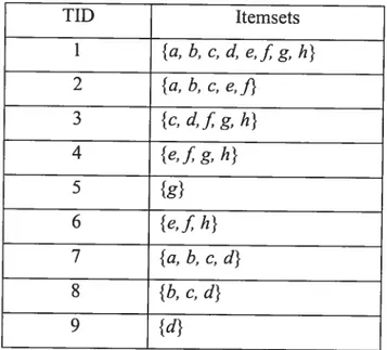
Assume 1= {a, b, e, d e,
f
g, h}A transaction set is as follows:
is a set of distinct items.
TTD Itemsets 1 {a, b, c, d, e,f g, h} 2 {a,b,c,e,f} 3 {c,d,fg,h} 4 {e,fg,h} 5 {g} 6 {e,fÏz} 7 {a,b,c,d} 8 {b,e,d} 9 {d}
(1, {a, b, e, d, e,
f
g, h}) and (8, {b, e, d}) are transactions, 1 and 8 are the TID of thesetransactions. The size of {a, b, c, d, e,fg, h} is 8, so {a, b, e, d, e,f g, h} is an 8-itemset. The
size of {b, c, d} is 3, so {b, c, d} is a 3-itemset. Since three transactions (#l, #7 and # 8)
contain itemset {b, e, d} and the total number of transactions is 9, soszipp ({b, c, d})
Definition 2-4: If the support of an itemset X is above a user-defined minimal threshold (nzinsttpp), then X is frequent (or large) and X is called afrequent itemset (FI).
for example: given minsupp 0.3
supp ({b, e, d}) = 0.3, so {b, e, d} is frequent (large), we calÏ {b, e, d}a
frequent itemset
sttpp ({a, b, e, e,) =
1
<0.3, so {a, b, e, e, is non-frequent (non-large).Rakesh Agrawal, Tomasz Imielinski, and Arun Swami proposed Property 2-1 and Property 2-2 in [Ais 1993].
Property 2-1: Ail subsets ofa frequent itemset are frequent.
Property 2-2: Ail supersets of an infrequent itemset are infrequent.
Definition 2-5: An association nue is an expression X=Y, where Xand Yare subsets of I, andXn Y= 0.
The stupportof a rule Xi>Y is Uefined as supp (X=>Y) sztpp (XuY). Thecoifidence ofthis rule is defined as co,f(X=>Y) sttpp (XY) /supp (X).
For example: {b, c} {d} is an association nue, sïtpp({b, c} {d}) =supp{b, e, d} co,f({b, c} {d})supp({b, e, d})/sttpp({b, c})= = =0.75.
Mining Dynamic Databases for Frequent Cosed Itemsets 6
Mining association mies in a given transaction set T means generating ail assciation mies that reach a user-defined minimal support (minsupp) and minimal coifldence (minconj. This probiem can be divided into two steps.
• Finding ail frequent itemsets.
• Generating association mies from frequent itemsets.
The generation of association ruies from frequent itemsets is reiativeiy straightforward tAS1994], since one divides a FI into two compiementary parts to make a mie between premise and conclusion. Therefore the research in the domain lias focused on determining frequent iternsets and their support.
2.1.2 Basics of concept lattices
Concept lattices are used to represent conceptuai hierarchies that are inherent in sorne data. They form the core ofthe mathematicat tlieory of Formai Concept Analysis (FCA) [W1982J. lnitialiy FCA was introduced as formaiization ofthe notion of concept, now it is a powerful theory for data analysis, information retrieval and knowiedge discovery [GW1999]. In Artificiai Intelligence, FCA is used as a knowiedge representation mechanism. In database theory, it has been used for cïass hierarchy design and management [SS1998, WTL1997]. In the Knowiedge Discovery in Databases (KDD), FCA has been used as a formai framework for discovering association mies [STBPL2000]; furthemrnre, it has been successful in improving the performance of aigorithms that mine association mies [PBTL1999-1].
The basics of ordered structures
Definition 2-6: Consider a set G and a, b, c G. A partial order on G is a reflexive (ae G
I
a a), anti-symmetric (a, be G a b & b a = a = b) and transitive (a, b,cE G a b & b e = a c) relation.
Definition 2-7: The set G in conjunction with an associated partiai ordering relation Gis
caiied apartially ordered set orposet or partial order and is denoted by (G,G).
Definition 2-8: Let P= (G,G) be a partial order. for a pair of elements, s, pe G, ifp G,
we shah say that s succeeds (is greater than)p andp precedes s. Ail common successors of s andp are called upper bounds of s andp. Ail common predecessors of s andp are called lower bounds of s andp.
Definition 2-9: Let P=(G,G)be a partial order and A be a subset of G, if there is an element
se G such that s is the minimal of ail upper bounds of A, then s is called the least zipper botind of A (LUB); if there is an elernent pe G which is the maximal of ail lower bounds of A, thenp is called the greatest lower bound of A (GLB).
Definition 2-1O:The precedence relation<Gin P is the transitive reduction ofG, i.e. s <Gp if s Gp and ail t such that s G tGp satisfy t=s or t=p. Ifs <G?, s will be
referred to as an immediate predecessor of p and p as an im,nediate sztccessor of s.
Usually, P is represented by its covering graph Cov (F) = (G, <G), also called the Hasse
diagram. In this graph, each elernent s in G is connected to both the set of its immediate predecessors and of its immediate successors, further referred to as Ïower covers (Cov’) and zipper covers (cov”) respectively.
Definition 2-11: If a subsetA of G satisfies V s,p eA, s Gp vp Gs,then the setA is called
a chain and the elements are said to be pair wise comparable.
Definition 2-12: If a subset A of G satisfies V se G, V peA, s Gp = seA, then the set A is
called an order icleat.
Definition 2-13: 1f a subset A of G satisfies V se G, VpeA, p Gs =seA, then the set A is
Mïning Dvnamic Databases for frequent Closed Itemsets $
Definition2-14: A lattice L= (G, L)is a partial order in whicheverypair of elements s,p has
an unique greatest lower boztnd (GLB) and an unique least upper bound (LUB). LUB and GLB define binary operators on G cailed, respectively, join (sVLp) and meet (s ALP)•
Definition 2-15: Given a lattice L= (G, L),ail the subsets A ofthe G have a GLB and a LUB,
we cal! this lattice a complete lattice.
Definition 2-16: A structure with only one ofthejoin and meet operations is calÏed a sein i—lattice.
The existence of a unique GLB for every pair of elements implies a meet semi-lattice structure and the existence of a unique LUB for every pair of elernents impiies a join serni-!attice structure.
Definition 2-17: A forma! context is a triplet K (T, I, R) where T, I are sets and R T x 1 is a binary relation. The elements of T are called transactions (or objects) and the e!ements of I items (or attribittes). Each pair(t, i)e R indicates that i is an item of transaction t.
Definition 2-1$: T, lare sets, the
(f
g) is a GaÏois connection between 2’ and 2’,f
2’— 2’, g: 2’—> 2’ iff, for alI XE2Tand YE2’,f(X) Yg(Y) c X.Definition 2-19:Let K = (T, I, R) be a formal context, the function
f
maps a set oftransactions onto a set of items that are common, whereas g is the dual function for the set of items.fand g are defined by’.
J(X)=X’= {ie IIVtetRi} g(Y)=Y’={tE TIVieY,tRi}
R.WiHe proposed Property 2-3 and Property 2-4 in [W 1982]. Property 2-3:
(f
g) is a Galois connection ofthe formai context.Property 2-4: Compound operatorsf°g(Y) andgoJ(X) are Galois clositre operators over 2’ and 2” respectively. Hereafter, both
f
0g (Y) and g°f(X) are expressed by“.f0gl)=f(g(Y))=
r’
gof(X)zzzg(f(X))=X’
Forexample: {e,fh}”=f(g({e,fh}))=f({1,4,6})= {e,fh}, {1, 4, 6}”=g(f({l, 4, 6})) =g({e,f Ïi}) = {1, 4, 6}.
X’ is the closure of X, which isthe srnallest closed itemsct containing X. For example: X= {a, b},
X’= {a, b}”= {a, b, c}.
Definition 2-20: An itemset Xis closed if X=X’.
If an iternset Xis closed, adding an arbitrary item i from I-Xto Xresulting a new itemset X which is less frequent [PHM2000].
Property 2-5: Suppose Xis closed, then V j I-X sttpp (Xu{i}) <supp (X). For exampie: X= {a, b, e, e,J}, 1-X {d, g, h},
2
Xis a closed itemset and supp ({a, b, c, e,J}) —.
supp({a, b, e, d, e,J})=supp({a, b, e, e,fg})
= supp ({a, b, e, e,
f
h}) =1<
.Every itemset lias the same support as its closure. This property lias been proven by [PBTL 1999-Ï]
Property 2-6: supp(X) = supp (X”).
Mining Dynamic Databases for Frequent Closed Itemsets 10
(fCI). Namely: fCI ={X Xe CIs Asupp (X) minsupp}. for example: given rninsupp=0.3,
{a, b, c} is a closed itemsct andsitpp ({a, b, c}) = > 0.3, so {a, b, c} is a
frequent closed iternset.
Definition 2-22: A concept c is a pair of sets (X Y) where Xe2T,
Ye 2’,
X= Y’ and YX’. Xis called the extentofconcept e and denoted byext(c), Yis called the intentofthe concept c and denoted by int(c).
For example: in Table 2-1, {1,2,7}’={a, b, c} and {a, b, c}’={l,2,7}, so ({1,2,7}, {a, b, c})
is a concept. {1, 2, 7} is its extent and {a, b, c} is its intent.
for a concept c (X
Y),
since X= Y ‘= {X ‘}‘= X’, so the intent of a concept is a closeditemset.
Definition 2-23: The support ofa concept equals to that of its extent, it is defined as follows.
XI
For a concept c = (X Y),supp (c) =
For example: in Table 2-1, ({1,2,7}, {a, b, c}) isa concept, sïtpp (({l,2,7}, {a, b, c}))=
Definition 2-24: If the support of a concept e is above a user-defined minimal threshold (minsupp),then e is frequent (or large) and e is called afrequent concept.
Definition 2-25: Let C be the set of concepts derived from a context. The partial order L = (C,t) is a complete lattice called a concept lattice. The partial order is
defined as folÏows.
A concept lattice L= (C, L) is a partial order in which
every
pair of concepts, cj, c2, has aunique greatest lower bound and a unique least upper bound. The binary operators on C denoted, respectively,join (CIVL C2) andmeet (ci ALc7)[W 1982]:
tXi, Y1) VL X2, Y2) ({X1UX}”, {Y1
n
Y2}),(X1, Y1) AL X2, Y2)= ({X1flX2}, {Y1 U Y2}”).
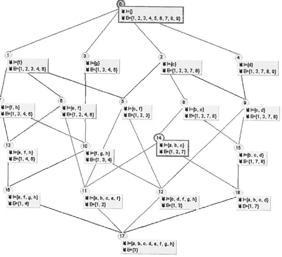
The Hasse diagram oftbe concept latticeL from Table 2-1 is shown in figure 2-1. Intents and extents are indicated in rectangles below the nodes. For example, the join and meet of c#5 ({l,2,3}, {c,J}) and c4= ({l,3,7,$,9}, {d) are c#o ({1,2,3,4,5,6,7,8,9}, Ø and cl2 ({1,3}, {c, d,f g, h}) respectively.
Two functions, p andv, are defined on the concept lattice. Definition 2-26: The functionp: T—L is defined as follows:
t(t) - A{Cj t ext(c)} = ({t}”, {t}’).
Given a transaction t, this function is used to find a minimal concept e (according to the size
of extent) in L and ext(c) includes the transactiont.
for example, within the concept lattice in f igure 2-l, p(2) = C#1I and p(6) c#13.
Definition 2-27: The functionv I— L is defined as follows: v(i) =
v{cI
jE int (c)} = ({i}’, {i}’’).Given an item i,
this
function is used to find a maximal concept e (according to the size of extent) in L and int (e) includes the item j.For example, within the concept lattice in Figure 2-1, v(d) = c#4 and v(J) =c#i.
Hereafter, tc denotes the set of ail successors of concept e (the order filter generated by e) and
Lc
denotes the set of all predecessors of concept e (the order ideal generated by c). The notion and properties of iceberg were introduced in [STBPL2000].Mining Dynamic Databases Ior Frequent Closed Itemsets 12
partial order (Ca, p) is called the iceberg concept lattice.
Property 2-7: Lais an upper-semi-lattice (orjoin-semi-lattice) of L.
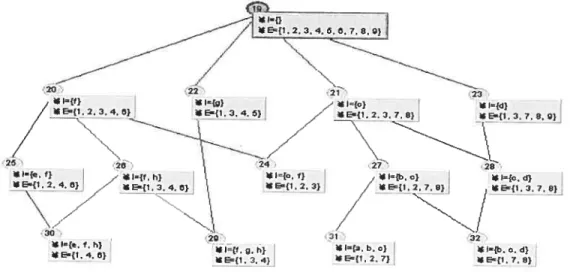
The set of ail a-infrequent concepts in L forms asub-semi-iattice (join-semi-lattice) of L. for example, given a minsupp a= 0.3, the iceberg lattice from Table 2-1 is shown in figure 2-2. The support ofeveryconcept in Figure 2-2 is greater than 0.3.
—z 2O / * t={f} / *E{1.2.3.4.8} *E{1.3.4.e} / I- -- - -/ ---/ J ----/ 1 24 1{e.f} /*I{f,h} *1{c,fJ
E{1.2,4,8} z *E{1,3.4.8} E{1,2.3}
/ ---ç---_ 30 l={. f. h) ,h) Ei.4.6} *E{1.3.4} 21 /•I=} E{1. 2,3,7. 8} N. 27 28 E={1.3, 7. 8]-31 32) *Ia. b. c} I{b. a. d} E={l.2.7}j
figure 2-2: The iceberg lattice L°3 from Table 2-l (a=O.3)
2.2 Current state of researcli on association mining algorïthms
Many algorithms for association mie mining have been designed, we can classify them into several categories.
2.2.1 Plain frequent itemsets mining algorithms
In 1993, Rakesh Agrawal, Tomasz Imielinski, and Arun Swami proposed the notion of an association mie and a corresponding aigorithm, caÏÏed Apriori, to discover ail significant association mies between itemsets in a large transaction set [AIS 1993]. Apriori is a famous atgorithm and enumerates every single frequent iternset. It uses the downward ciosure property of itcmsets support to prune the search space-ail subsets of a frequent itemset must
be frequent. Only the frequent k- itemsets are used to construct candidate (k+Ï)-itemsets. A pass is executed over the transaction set to find the (k+])-frequent itemsets from the (k+ 1)-candidates.
Many variants of Apriori achieve improved performance by reducing the number of candidates. Some algorithms reduce the number of transactions to be scanned [AS 1994,
_,_z- / l—ti.z3. 4.5.e,7,8.oH
—z- /
-RI={d}
Mining Dynamic Databases for Frequent Closed Itemsets 14
HF1995, PCYÏ 995] and sorne reduce the number of transaction set scans [BMUT1997, S0N1995, T1996].
FP-growth is anther well-known algorithm which finds complete frequent itemsets [HPY2000]. It first constructs a compressed data structure,frequent-pattern tree (fF-tree),
to hoid the entire transaction set in memory and then recursively builds conditional FP-trees to mine frequent pattems. FP-tree is an extended prefix-tree structure and ail transactions with the sarne prefix share the portion of a path from the root. FP-growth algorithm avoids the problem inherent to candidate generate-and-test approach, thus its performance is reported to be better than that ofApriori. However, the number ofconditional FP-trees is in
the same order of magnitude as number of frequent itemsets. The aigorithm is not scalable to sparse and very large transaction sets.
2.2.2 frequent cfosed itemsets mining algorithms
frequent itemsets mining oficn generates a large number of frequent itemsets and mies. This process reduces the efficiency ofmining since one has to filter a large number of mined mies to get useful ones. A-close aigorithm is an important alternative that was proposed by N.Pasquier, Y.Bastide, R.Taouil, and L.Lakhai [PBTLÏ999-2]. It uses ciosure operators to caiculate the frequent ciosed itemsets and their corresponding mies.
As a continued study on FP-growth, [PHM2000] proposed CLOSET. It is another efficient aigorithm for mining frequent closed itemsets based on fP-tree. The special features of this particular aigorithm are the three techniques deveioped for the purpose of complexity reduction. first, CLOSET appiies an extended frequent-pattem tree to mine ciosed itemsets without candidate generation. Secondly, to quickly identify frequent closed itemsets, it develops a single prefix path compression technique. Finally, this scheme explores a partition-based projection mechanism for pattems on subsets of items.
CHARM [ZH2002j is another efficient algorithm for mining ail frequent closed itemsets. This algorithm implernents a hybrid search technique, called dual itemset-tidset search tree (IT-tree) which enables it to skips many leveis of the IT-tree to locate the frequent closed
itemsets quickiy. A fast hashtabte-based approach is also used in order to remove non-closed sets found during computation.
In a sparse transaction set, the rnajority of frequent itemsets are ciosed iternsets. The performance of A-Close is therefore close to that of Apriori. The advantage of CLOSET over A-Close is essentially the same as that of FP-Growth over Apriori [PHM2000]. In this kind of transaction set, CHARM also outperforms Apriori due to the fast hash-table and the dual iternset-tidset search tree. If the minsupp is srnail and the TID sets for frequent iternsets are smail, CHARM wiÏl be efficient. However, its performance is inferior than that of CLOSET since CLOSET employs the closure mechanism on a more elaborate scale. The benefit of CLOSETbecomes even more significant on dense transaction sets, since CLOSETonYy scans the transaction sets twice and the mining process is confined to the frequent pattem tree after that. Also, regardÏess ofhow many times the transaction sets are being iterated, the frequent pattem tree maintains the same shape with respect to the constant rninsttpp. Hence, the runtime of CLOSET over real transaction sets increases at a much siower rate than that ofthe sizes of transaction sets [PHM2000].
A recent algorithm TITANIC [STBPL2000] is another algorithm based on Galois connections for mining frequent cÏosed itemsets. It is inspired by the Apriori algorithm, as well as adopts a more powerfiil pruning strategy. This strategy determines the support of ail k-itemsets that remain at thekth? iteration, and computes the closure of ail (k-1) -itemsets afier
the (k_1)th iteration.
2.2.3 incremental FI or FCI mîning algorithms
The most important problem with association mining is the huge number of frequent itemsets and association rules that can be generated from a iarge transaction set. The methods based on the frequent closed itemsets are a promising solution to the problem of reducing the number of association ruies. However, confronting a dynamic transaction set, another problem arises since the transaction set is frequently updated. Adding new transactions may invalidate existing frequent pattems or generate new ones, thus one needs to re-execute the
Mining Dynamic Databases for Frequent Closed Itemsets 16
algorithms from the beginning. So far, a few incremental aÏgorithrns for association mining have been proposed [GMAY 995, CHNW 1996, STBPL2000, VMG2002].
[VMG2002] proposed an incremental algorithm for mining frequent closed itemsets based on lattice construction (GALICIA). The difference between it and other FCI-based techniques is: it avoids reconstructing the frequent closed itemsets completely when transactions are added to the transaction set and / or the ni insupp is changed. However, as mentioned earlier, it is inefficient since one needs filter frequent closed itemsets from closed iternsets.
2.3 Review of two typical algorithms
In this section, we review two best-known association ruÏe algorithms: Apriori, a plain frequent itemsets mining algorithrn, and A-Close, a frequent closed itemsets mining
a}gorithm.
2.3.1Apriori algorithm
Apriori algorithm uses Property 2-1 and Property 2-2. It performs a number ofiterations. In each iteration (i), it first constructs a set of candidate itemsets based on frequent itemsets
obtained from the preceding iteration(i-J);then scans the transaction set to filter the frequent i-itemsets.
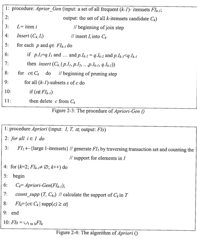
The procedures used in the Apriori algorithm are shown in Figure 2-3 and Figure 2- 4 (Ck represents the set of candidate k-itemsets, fIkrepresents the set of frequent k-itemsets).
Aprior_Gen() is a sub-function of the algorithm. It generates the candidate itemsets by joining the frequent itemsets ofthe previous pass that have the same items except for the last one, and then generated candidates that contain an infrequent subset are dropped.
Apriori
()
is the main procedure of the Apriori algorithm. It has three main steps. First, it considers the itemsets with only one item (unes 2-3) and calculates frequent ]-itemsets. Secondly, it executes an iterative process, calling Aprior GenQ, to get the frequent itemsets(unes 4-9). This iterative process terminates when no new frequent itemsets can be found. Finally, ail frequent itemsets are accumulated (une 10).
1: procedure: Aprior Gen (input: a set of ail frequent (k-1)- itemsets F1k1;
2: output: the set of ail k-itemsets candidate Ck) 3: I= item i II beginning ofjoin step
4: Insert(Ck,I) II insert L into Ck
5: for each p and qe f1k/do
6: if p.I=q.I and ... andp1k2 q.ik-2 andp.1k]<q.Ik1
7: then insert (Ck(pJI,p.I2, .. q.I))
8: for ce Ck do II beginning ofpntning step
9: for ail (k-1)-subsets s ofc do
10: if(sEflkJ)
11: thendelete cfromCk
Figure 2-3: The procedureofApriori-Gen
O
1: procedureApriori(input: I, T a output: FIs) 2: Jorail je I do
3: fI, —{1arge i-itemsets} // generateFI,bytraversing transaction set and counting the
II support for elements inI
4: for (k=2; F1k1 0; k++) do 5: begin
6: Ck= Apriori-Gen(FIkJ);
7: cozmtsupp (T Ck,) II calculate the support ofCkin T
8: FIk={ceCk(supp(c) a} 9: end
10: FIs= u1to kf’k
Mining Dynamic Databases for frequent Closed Itemsets 1$
for example, according to the transaction set in Table2-1, FI2 ={{a, b}, {a, c}, {b, c}, {b, d},
{c, d}, {c,J}, {e,J}, {e, h}, {fg},
1f
h}, {g, h}}, afterthejoiningstep inApriori-Gen , C3wiIl be {{a, b, c}, {b, c, d}, {c, d,J}, {e,f h},
{f
g, h}}. The prune step will delete {c, d,J} because itemset {d,J} is not in FI7, so C3 is left with{
{a, b, c}, {b, c, d}, {e,f h},1f
g, h}}.
After calculating their supports by traversing the transaction set, we get FI3={
{a, b, c}, {b, c,d}, {e,f h}, {fg,h}}.
According to the experimental resuits, Apriori outperforrns other plain frequent itemset mining algorithms [AIS 1993]. Since its introduction, two enhanced versions of Apriori algorithms were developed: Apriori-TID [A1S1994] and Apriori-Hybrid [A1S1994]. The main difference between Apriori and Apriori-TID is that Apriori scans the entire transaction set in each pass to count the support in order to discover frequent itemsets. Apriori-TID does flot use the transaction set for counting support after the flrst pass. It employs an encoding of the candidate itemsets used in the previous pass. Apriori-Hvbrid algorithm is a combination of Apriori and Apriori-TID. As mentioned in [AIS 1994], Apriori has better performance in earlier passes; Apriori-TID has better performance in later passes. Apriori-Hybrid technique uses Apriori in the initial passes, and switches to Apriori-TID for the later passes if necessary. Apriori-Hybrid technique improves the performance greatly.
2.3.2 A-Closealgoritlim
A-Close is a non-incremental algorithm for mining frequent cÏosed iternsets which is inspired by Apriori algorithm.
The A-Close algorithm contains several main procedures. The first is the AC-Generator function, which is based on the properties ofclosed itemsets. It determines a set ofgenerators. Here the generator is defined as folïows: an iternsetp is a generator ofa closed itemset e if it is the smallest itemset that will determine e using the Galois closure operator: p” = c.
[W19$2]. In this procedure, it applies Apriori-Gen
Q
to the i-generator set to obtain the (i+])-generator candidate set. It joins two i-generators with the same first i-1 items to produce a new potential (i+])-generator, afler getting (i+1)-generator candidates, theirsupports are calculated, then the infrequent (i+1)-generators and (i+])-generators that have the same closure as one oftheir i-subsets are discarded.
The second is the A C-Ctosure function. Once ail frequent generators are found, they will help us to get ail frequent cÏosed itemsets by using Galois closure operators “. In order to reduce
the cost ofthe closure computation, A-Close aigorithm adopts an optirnized pruning strategy by locating a (i+1)-generator that was pruned because it had the same ciosure as one of its i-subsets to start the first iteration. Ail iterations before i11, the generators are closed, SO it is
unnecessary to carry out the closure computation for them, and then we just perform the closure computation for generators of size greater or equal to i. For this purpose, the algorithm uses the level variable to indicate the first iteration for which a generator was pruned by this pmning strategy [PBTLY999-2].
A-Close algorithm finds the candidate generators during iterations. It is necessary to traverse the transaction set to calculate the support for the candidate generators. 1f a generator is flot cÏosed, it will require one more pass to determine its closure; if ail generators are cioscd, this pass is flot needed.
for example, from transaction set in Table 2-1, A-Close algorithm discovers the FCIs as follows withminsupp=0.3. First, the aigorithm discovers the set of 1-generators, G1 and the
support for each elernent, no generator is deleted, because ail are frequent. Then 2-genetators in G2 are detenuined by applying the AC-Generators function to G1, ail infrequent 2-generators are pmned (ail infrequent 2-generators are flot shown due to the limitation ofthe space), meanwhile, {a, b}, {a, c}, {e,J} and
{f
h} are pruned since supp({a, b})=supp({a}), supp({a, c})= supp({a}) , supp({e,J}) = supp({e}) and sïtpp({f Ïz})=supp({h}). The levelvariable is set to 2. Calling AC-Generators function with G2 to produce G3, we get {b, c, d} and {c, d,
J},
but {b, c, d} is pruned since supp({b, c, d})
= supp({b, d}) and {c, d,J}
ispruned since {c,
J}
G2. At last, since the levet variable is 2, so the candidate generators G’ inciudes the generators from G1 and G2, the closure function AC-Ctosure is appiied to G’ to discover the ciosures of ail generators in G’ and duplicate closures are removed from G’, vie get ail frequent closed itemsets. Figure 2-5 illustrates the whoie process.Mining Dynamic Databases for Frequent Closed Itemsets 20
G1 G1
Support_count Generator Support Pruning Generator Support
{a} 3 infrequent {a} 3
{b} 4 generators {b} 4 {c} 5 {c} 5 {d} 5 {d} 5 le} 4 {e} 4 {!} 5 {R 5 {g} 4 {g} 4 {h} 4 {h} 4
G2 (ail frequent 2-generators) G2
AC-Gencrator (a,b} 3 Pnining {b,c} 4
(a,c} 3 {b,d 3 {b,c} 4 {c,d 4 {b,cl} 3 {c,J} 3 {c,d} 4 {e,h} 3 {c,f} 3 {fg} 3 {e,/} 4 {g,Ïz 3 {e,h} 3 {fg} 3 {fh} 4 {g,h} 3 G3 G3 AC-Generator {b,c,d} 3 Pruning {c,d,J} 2 G’ FCIs
Generator closure support Pnrning Closure support
AC-Closure {a} {a,b,c} 3 {a,b,c} 3
{b} {a,b,c} 3 {c} 5 {c} {c} 5 {d} 5 {d} {d} 5 {e,f} 4 {e} {e,f} 4 {/} 5 {J} {/} 5 {g} 4 {g} {g} 4 {fh) 4 {h} {/h} 4 {b,c} 4 {b,c} {b,c} 4 {b,c,d} 3 {b,d} {b,c,d} 3 {c,d} 4 {c,d} {c,d} 4 {c,J) 3 {c,f) {cJ} 3 {e,fÏi1ç 3 {e,h} {e,fh} 3 {fg,h} 3 {fg} {fg,h} 3 {g,Ïî} {fg,h} 3
After studying above algorithms, in this thesis, we explore the problems of mining frequent cÏosed itemsets. We attack these problems by implementing our proposed algorithm—ILA
(Iceberg Lattice Algorithrn). ILA algorithrn takes advantage of incrernental methods and
maintains only the upper most part of a concept lattice. As a critical feature, ILA algorithm improves the efficiency of frequent closed itemsets mining by avoiding useless computation and taking advantage ofthe previous iceberg structure. NameÏy, we improveILA by (1) only scaiming the transaction sets once and (2) only storing current frequent closed itemsets when a new transaction is added.
Mining Dynamie Databases for Frequent Closed Itemsets 22
Chapter III Review of the GALICIA approach
GALICIA is a farnily of algorithms that generate frequent closed itemsets incrementally. Its aim is to construct new closed itemsets based on current family ofclosed itemsets by looking on the new transaction t+j. The incremental construction of the concept Ïattice may help design the effective methods for frequent closed itemsets mining.
3.1 Lattice updates
Incrernental rnethods construct the concept tattice L starting from the initial lattice L0= ({Ø I}, 0). When adding a new transactiont1+1, we incorporate it into the concept lattice L. Each
incorporation causes a series of structural updates. The basic approach was defined for concept lattices [GMA1995] and was improved upon latcr [VM200Y]. It is based on the fundamental property ofthe Galois connection established byfand g on (T, 1): both families ofclosed subsets are themselves closed under set intersection [BMÏ 970]. So when inserting a new transaction t+j,we shouid insert into L ail new concepts wliose intent is the intersection of {t1+1}’ and the intent of an existing concept where the intersection is not an already
existing intent.
We now define a mapping
y
that Ïinks the concept lattices L and L1+1. The mapping y sends everye from L1+1 to the concept from L1 whose extents correspond to the extent ofemodulotï+1.
Definition 3-1: The mappings y: C÷j—> C are established as follow. y(X Y)=(Xi,Xi’),whereXi=X- {t+1}.
Ail concepts in L can be ciassified into three categories (hereafier C and C+1 denote the sets of concepts in L1 and L1+1 respectively).
Genitor concepts (G(t1+1))-- generate new concepts by intersecting with new transactiont1+j
and help calculate the respective new intents and extents. Definition 3-2: The sets ofgenitor concepts in L1+1 and in L1 are
G(t+1)= {cr=(X Y’)
I
Y{
t1+i}’; Y=(Yn{
t1+j}’)”} respectively.Modified concepts (M(t1÷j))--their intents are included in the new transaction’s itemsets, so
their intents will remain stab’e, only the lTD ofnew transactiont+1 is integrated into their extents.
Definitïon3-3: The sets ofmodified concepts in L1+1 and in L are W(t1+1) = {c =
(
Y)J
ce«; t1÷j e (X- {t1+1}’) — Y},{c (X Y) j ceC, e e M( t1+ï), c y(e)} respectiveÏy.
Old concepts (O (t1+1)) -- remain completely unchanged when adding a new transaction t1+j.
Definition3-4: The set of new concepts in L1+1 is
AQ1+1)= {{c(
Y)
ce C1±1; t1+j e X; (X- {t1±1})” =X- {t1+1}}.The incremental algorithms focus on a substructure ofL1+1 that contains ail concepts with t+’
in their respective extents, i.e. both new concepts, PJ( t+) and M( t+1). We regard this structure as an order filter, which is generated by the transaction-concept of t1+j in L1÷1,
denoted by p (t1+1). The order filter tp (t1÷1) induces a complete sub-lattice of L1+1. The
choice of a pivotai structure is determined by the isornorphic structure in L1, which is cornposed of G(t1+1) and MQ1÷1). Thus when A’( t1+1) is integrated into L, the desired links
can be inferred from the structure isornorphic to t1tt(t1+1)within L.
In order to generalize the intersections ofthe description oft1÷j and the entire set C, we define a mapping that links L to the lattice of the power-set of ail attributes, 2’.
Definitïon 3-5: The function
Q:
C— 2’ computes: Q(c)= Yn {t1+1}’.The function
Q
induces an equivalence relation on the set C, and the class of a concept c is denoted by [clQ. The set ofequivalence classes C/Q is considered together with the following order relationMining Dynamic Databases for Frequent Closed ltemsets 24
Since the intents of concepts in tct(t1+1) are ail subsets of{t1+1}’ which are closed in K, the
resulting partially ordered structure, L/Q, is isomorphic to
tp
(t+1) and is a complete lattice. The following algorithm (see figure 3-1) is a generic scheme for the incremental task. It detects the three categories of concepts with the creation of the new concepts and their subsequent integration into the existing lattice structure [VM2001].This algorithm takes a lattice and a new transaction as arguments and outputs the updated lattice using the same data structure. It includes three main computation steps. The first step is a traversai of the set L with a simultaneous catculation of the intersections between the respective concepts and the itemset ofthe new transactiont1+1 (i.e. {t1+j}‘), the partitioning of
L into classes with respect to
Q
(une 3-4), and the detection of classmaximal concept
for every class []Qwith the subsequent identification ofthe status ofthe maximal element (unes 5-6). Secondly, it deals with modified concepts (unes 7-8). It updates their extents and increases the corresponding supports. Finally, it deais with the genitors (unes 10-14). It includes the creation ofa new concept and the order update in the lattice [VHM2003].1: procedure
add-traizsaction
(In / Out: L a lattice, t1+j a new transaction) 2:3: forallcinLdo
4: put
c
in its class in L/Q w.r.t.Q(c)
5: for ail[]
in L/Q do6: find
e
max([])
7: ifint(e)
C{
t1+1}’ then8: add (ext (e), t1+1) {e is modified concept} 9: else
10: int —
int
(e) n{
t1+1}’ {e is old or potential genitor}11: if(not (int’, int) e L) then
12:
{ e —New-Concept (ext
(e) ut+i, int) {e is genitor}13: Update -Order (e, e)
14: add(L, e)}
for example: we take the third transaction out from Table 2-l, we get Table 3-1: TID Itemsets 1 {a, b, e, d, e,
f
g, h}
2 {a,b,c,e,J} 4 {e,fg,h} 5 {g} 6 {e,fh} 7 {a,b,c,d} 8 {b,e,d} 9 {d}Table 3-1: An example of transaction set with $ transactions Following the above algorithm, we get concept lattice L8 as figure 3-2.
— _—--
//
f) *l— * —{b.y) * E-1.2.4.8J / -{t 2O -{l.7. 0. 9) - \_____/
—--/
i• — E—1 4 \ — L ç_. l.2.7): .-. — —- \ *I.Y g.r} t. cd)E—t1,2 *E-{I.4) E-f1, 7)
-j_—
-17-
-*1a,b, C. d,e,1,gb)
Mining Dynamic Databases for Frequent Closed Itemsets 26
When adding a new transaction 3 = {c, d,f g, h} to Table 3-1, transaction set T is the same
as Table 2-1. When inserting the transaction 3 to L8, three categories of concepts are: 1. 0M concepts= {C#14, c918}
2. Modified concepts = {c#o, c, c#3}
3. Genitor concepts= {c98, C#6, c15, c3, c1, C#16, C#17}
The new concepts {c#i, c2, cfl5, c7, c9, C#io, c#12}
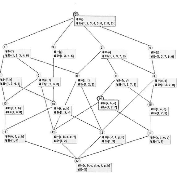
Integrating new concepts into L8, we can get new concept lattice L9 as Figure 3-3.
* I={g} //*1{c} * h{d}
*{1.234.6}ç *E{1.3,4. *Ec{1.2378} *E{1.3,7,8.Q}
7 7/
j
‘.. --I—-—-- 7/ / N J / N 8 0:*I=1h} ,Z *Ie.f} *Nc.f} /•*Itbc} 7 *Ic.d}
*E’{l 3 4 6} *E={1 2 4 6}
/
*{1 2 3) / *{I 2 7 8) / *E={1 3 7 8)- — /1 //
/
\Z
/ J/
\
r- ,// , J / w / -z*1{a b. o) I ,/‘*te,th) \._*1{f,g,h) /ç
IfiLUU
/ *I={b.o.d}*E={I,4.61 *{1.3.4) _7 *Ec{I7.8}
/
//
*1{ef.g,h) *1{a,b.o.e.t) ,‘ *Io.d.t.g.h)
-- *E412} --- /7 *E=f1.3) *E={1,7)
Z
// ____-*Iqa,b.o.d.e,f,g,h) *E{1)3.2 GALICIA family 3.2.1 GALICIA scheme
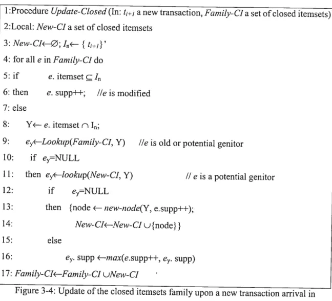
There are several differences between lattice update and closed iternsets update. Here, ciosed itemsets is a set of intents of concepts, and there is no order between the elements. When one updates closed iternsets, only the intents and supports are used. Lattice update should consider the ordered link among the concepts. The algorithm in Figure 3-4 can help us understand the characteristic of this approach {VM200 1].
1 :Procedure Update-CÏosed (In: t+j a new transaction, fanziÏy-C1 a set of closed iternsets) 2:Local: New-CIa set ofcÏosed iternsets
3:New-CI—Ø;I<—
{
t+1}’4: for ail e in Farnily-CI do 5: if e. itemset c I
6: then e. supp++; lie is modified 7: else
8: Y<— e. itemset n I;
9: e<—Lookttp(Famity-CI, Y) lie is old or potential genitor 10: if e=rNULL
il: then e1—Ïookup(New-C1, Y) // eis a potential genitor
12: if e=NULL
13: then {node —new-node(Y, e.supp++);
14: New-CI<--New-CI u{node}}
15: else
16: e. supp <—rnax(e.supp++, e. supp) 17: Family-CI’—Family- CI uNew- Cl
Figure 3-4: Update ofthe closed itemsets family upon a new transaction arrivai in GALICJA aigorithm
Every closed itemset is examined in order to establish its specific category (modifled, oid or genitor). Modified ciosed itemsets simply get their support increased (une 6). Oid ones
1’1ining Dynamic Databases for Frequent Closed Itemsets 28
remain unchanged (une 8-9). Actuaily, every new closcd itemset is stored together with the maximal support already reached for it, i.e. since multiple cÏosed itemsets can generate the same cÏosed itemset with different support, the current support is the maximal support ofthe new closed itemset, but flot yet confirmed that it is the maximum support for this closed itemset, thus each time the closed itemset is generated (une 11- 16), the support is tentatively updated. Furtherniore, the storage ofnew closed itemsets is organized separately (New-Cf), so that unnecessary tests can be avoided. This computation yieids the correct support at the end of closed itemsets traversai. Genitors are closed iternsets with maximum support of ail closed itemsets that generated new closed itemsets. This fact is strongly remforced by an implernentation that utilizes trie structures to reduce redundancy in both the storage and the update ofthe closed itemsets.
3.2.2 GAL1CIA-T
GALICIA-T is a version of GALICIA based on tries [K1998]. In generai, the trie data structure is used to store sets of words over a finite alphabet. It is a tree structure in which letters can be assigned to edges. Each word corresponds to a unique path in the tree. Ail nodes can be ciassified into two categories. One category compiles the terminal nodes that correspond to the end ofwords. The other category compiles inner nodes that correspond to prefixes. Trie offers high efficiency storage. Ail prefixes common to two or more words are represented only once in the trie. As a consequence, a trie reduces the storage space and manipulation cost. We can regard an item as a letter and an itemset as a word.
In GALICIA-T, one can implement two tries to represent the closed itemsets where one trie for the current closed itemsets family(Family-Ci), and the other for the new closed itemsets (New-CI). A node denotes a record withitem, terminal, successors, supportand depth fields. item provides the item in noUe and represents transactions and individuaÏ closed itemset. Successors is a sorted, indexed and extendable collection for lookup, order-sensitive traversai and insertion ofa new member. Terminal indicates whether the node is terminal, Le. whether Ycu,r, the current intersection between a closed itemset and I,, represents a closed itemset. Support records current node support. Depth is the length ofthe path from the root to node. The new transaction with its itemsets1,1is denoted by t1+;.
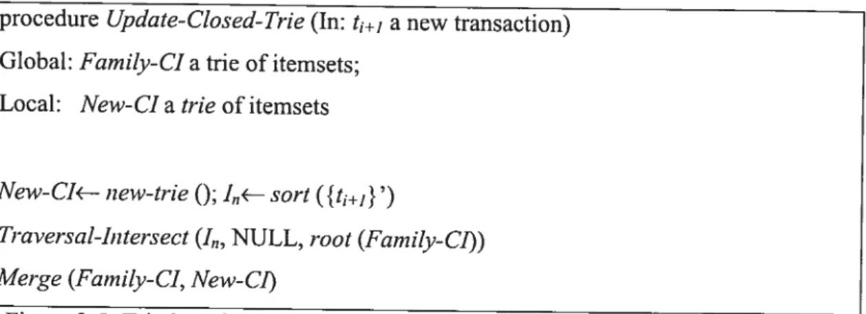
The algorithm in figure 3-5 describes die main steps of an update with a single new transaction t1+1. first, it creates a new trie to store the new closed itemsets, secondiy, it sorts
the {t1+j}’, thirdly, it traverses the trie and generates new closed itemscts, finally it merges
both tries.
1: procedure Update-CÏosed-Trie (In: t1+j a new transaction) 2: Global: Farnily-CI a trie ofitemsets;
3: Local: New-C’I a trie ofitemsets 4:
5: New-C1’1—- new-trie
Q;
Ifl—sort({t1+1}’)6: Traversal-Iiitersect (I,,, NULL, root (Fainity-Cf)) 7: Merge (Family-CI, New-CJ)
Figure 3-5: Trie-based update ofthe closed itemsets upon a new transaction arrivai The algorithm in Figure 3-6 is a recursive procedure that describes the simuitaneous traversai (with detection of common elements) oftwo sequences of items. Each trie traversai starts from the root and goes to a terminal nodc. If the cunently generated intersection (Y,,,.,.) is a new closed iternset, then we insert it into the New-CI trie; if it is aiready in the basic farniÏy-C1 trie, then we update the current node support. If the Iength of the current intersection,
IYc,,,.rI,
equals the depth ofthe current node, the second case occurs. It means that the current closed itemset ofthe trie is a modified element of L. An intersection is finished whenever a terminal noUe is reached. The resulting intersection is tested for being new (une 7), if it is the case, it is added to the New-CI trie (line 9), else it is an existing itemset, so it corresponds to a modified. b know whether the itemset that is cunently examined is the modified or it is just an old from the same equivaient class, one tests the equality of the size ofthe intersection to the size ofthe current itemset, i.e. the depth ofthe node in the graph of the trie. If the node has successors, the intersection goes on.Figure 3-7 depicts the resuit of the entire trie traversai. On the lefi, the state of FarniÏy-CI before the insertion of transaction 3 is shown. On the middle, the New-CJ is shown, and on the right, the situation of Family-CI afier insertion of transaction 3 is shown [VMGM2002].
Mining Dynamic Databases for frequent CIosed Itemsets 30
Figure 3-6: Trie-based update ofthe closed iternsets: single noUe processing
Family-CI a o_ O o4 •o 03 b I o 40 ô4 d 3 30 9 30 d, ef h 20 02 20 efgh 1 New-CI 5 ‘5 d f g 4 è3
6
4’0 fgh/ hi c3 Family-CI e f g4 o 0 b50 40 C 5Ô O b C d f .f gril 4o 40 03 4o 0 04 c d fgh g h h 30 30 20 0 03 ô3 d \ef h 20 02 2 efgh 10figure 3-7: Left: The trie Family-CI ofthe closed itemsets generated from T.
Middle: The trie NewCI ofthe new closed itemsets related to transaction #3. Right: The trie Family-CI after the intersection of transaction #3.
1: procedure Traversal-Intersect (In: I,, item-lists, node a trie node)
2: Global:farnily-CL New-CJtries ofitern-lists
3:
4: if (J,NULL) and (J,1.item= ,tode.itern)
5: then add I.item) 6: if node.terminal
7: then n <—Ïookttp(fanzily-Ci, Y11,.,-)
8: if n=NULL
9: then update-insert(New-C’I, Y,,,.,., node.supp++) 10: else
11: if node.depth=iY11.,.I
12: then n.supp++
13: if (not node.terminal) or (I,,NULL) 14: thcn
15: for all n in node.successors do
16 while (I,,NULL) and (I,1.item <n.item) do 17: I,1—I,,.next
The following table illustrates the advancement of this algorithm on one branch of the trie, {a, b, c, d, e,f g, h}, upon the insertion ofthe item list {c, d,f g, h}.
node.item terminal support
a {c, d,
f
g, h}
NULL N-b {c, d,
f
g, h} NULL N-c {c, d,f g, h} {c} Y 4
d {d,fg,h} {c,d} Y 3
h {h} {c,d,fg,h} Y 2
The first column is the items in a node, the second one is the value of I, (available part of
{
t+j}’), the third coÏumn represents the current result of the intersection, and the fourth oneindicates whether a node is terminal, i.e. whether the value of Y,,.r represents a ciosed itemset, the fifth column records, whenever reaching a terminal node, the value of the support. Incrementality is a major breakthrough in data mining methods and GALIC’IA is one of the flrst algorithms to adopt this method. The experimental resuits indicated its advantages for small rninsupp cases. However, the efficiency of the algorithm is hindered by the requirement to preserve ail closed itemsets. One solution of solving the dilemma is by maintaining only crucial parts of the closed itemsets (e.g. the frequent closed itemsets) and work on each particular set separately. So in our algorithm (ILA), we store only the part above the threshold in closed itemsets, which improves the performance.
Mining Dynamic Databases for Frequent Closed Itemsets 32
Chapter IV Maintain iceberg latfice only with FCIs
4.1 Incremental iceberg lattice update
The algorithms mentioned in section 3.2 can be used to compute frequent closed itemsets. There are two steps in the process: the first step finds closed itemsets from transaction sets; the second step filter the frequent ones with a defined rninsupp û’. The concept lattice L
contains ail closed itemsets. In previously mentioned algorithms, during the process of updating concept latticeL,we ignored the value of lninsupp û’. Once given aminsupp,we can
divide L into two parts. An upper part, denoted as La= K), where all concepts have supports greater than or equal to minsupp û’. We cal! it an iceberg lattice. For example, f igure
-i is an iceberg latticeL°3 from the complete concept lattice with a= 0.3; similarly, a lower
part, denoted asLa= (C K). In this way, we shouÏd be able to maintain (store and update)
ail closed itemsets, even if some closed itemsets are infrequent.
However, there are two disadvantages in these algorithms. One is that we must travel through ail closed itemsets when adding a new transactiont+i. Atso we must calculate the support for
every closed itemset to find frequent one. These two procedures increase the computational cost. Now, we will propose a nove! algorithm that only executes a few operations to maintain an existing iceberg lattice without excessive computations. These operations are based on the current iceberg lattice structure.
Given a contextK, iceberg lattice Lais the part above the threshold aofthe complete concept
latticeL of K. After adding a ncw transactiont1+j toK, an incremental algorithm executes the
same operations as with a complete lattice (add-transaction
o,
see section 3.1) to maintain the structural integrity of an iceberg Ïattice L° [VMG2002]. However, there are some additional tasks, such as eliminating ail concepts which become infrequent in L (L is constructed with the transaction set in K+ t1+j) and adding some concepts which are flotfrequent in L, but when adding a new transaction t1+j to their extents (e. g., modified concepts), they become frequent in L, or new frequent concepts in L which are produced by non-frequent genitors in L. So the maintenance of an iceberg lattice includes flot only creating new frequent concepts, but also deleting some old ones.
I{a.bc}
IE{1. 2, 7}
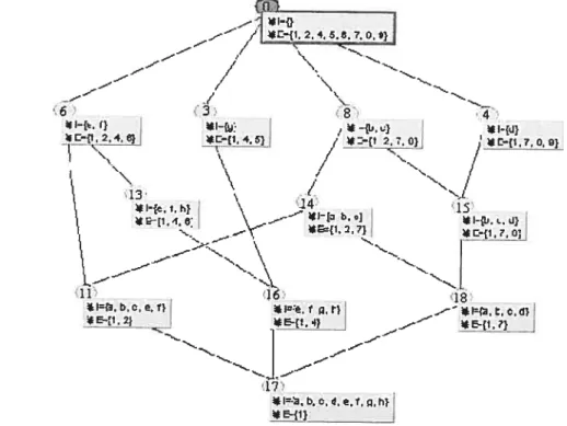
figure 4-l: The iceberg lattice L°3 with T= {1,2,4,5,6,7,$,9} & a 0.3
For example, Figure 4-lis the iceberg lattice L°3, after adding the new transaction 3, the new iceberg lattice L°3 is as Figure 4-2 and the respective concept categories are as follows. Old concepts= {c#31
}
Modified concepts = {c#22, C#23}
Genitor concepts = {c#25, C#27, C#30, c#32}
The new concepts inL°3= {c#20, c21, C#26, C#28}
/ N
//
/ t) I{g} ,‘ I{c} Id)
/ E{l,2,3,46] E—{1,3,4,5} / aE{l.23.7,8}, *E{1.3.7.8.9I,
2 \24
/
/
I—{e f) it h) 1{ f) I { ) I h d}
*E{1 2 4 )J / 3 4 E{l 2 3) // E{I 27 8) E{I 3 7 8)
‘\
//
/
/
/
I)e. f.h) *fr). b,o) IIIb. o. d)
E{1 .4. 6 E{t. 3 4J *E{1, 2. 7) E{1.7, 8)
*1{g} _—‘ *1{b.c} /.°{1.1fL. .-,----,- _I___,,.2}
/
/
/
32 II={b, cd) E{1.7.8)Mining Dynamic Databases for Frequent Closed Itemsets 34
4.2 Theoretical development
Our objective is to produce and maintain an iceberg lattice that only includes frequent closed itemsets. When adding a new transaction t+1, we should consider every element in iceberg
lattice L°. In this section, we present a new incrernental method to maintain the integrity of the iceberg lattice.
Variable Stands for
c A concept in La
T A transaction set
77 The number of transactions in T
TJ
The number of transactions in T+ t+1a Minsupp
L Complete concept lattice constructed with transaction set T La Iceberg lattice constructed with transaction set T and threshold
support a
La The “lower” part ofthe lattice with transaction set Tand threshold support
a
t1+j New transaction or the TID ofnew transaction
{t1±1}’ The itemsets ofnew transaction t+j
L Complete concept lattice constructed with transaction set T+ t1+1 La+ Iceberg lattice constructed with transaction set T+ t1+j and
threshold support a
La The “lower” part ofthe lattice with transaction set T+ t+j and threshoÏd support a
Table 4-l: The meaning of variables in ILA
According to the category of a concept, we must consider the outcome of each case and subsequently prove the resuit.
Let c be a concept in iceberg lattice (La) and t+j is a new transaction. If e is a modified
concept, then e (ext(c)u t+j, int (e)) is stiil a frequent closed itemset, it wiÏl be in the new iceberg lattice (L).
Property 4-1: Vc L° ifint(c) c {t+1}’ then e (ext(c) u t1+1, int (c))e La’+
for example, in Figure 4-1, when add the new transaction 3 = {c, d,
f
g, h}, e22 and c#23 arernodified concepts, i.e. int(c#72) c {c, d,f g, h} and int(c#23) ci {c, cl,f g, h}, so c#22 and cp3 are in Figure 4-2.
Let e be a concept in iceberg lattice (La) and t1+j is a new transaction. If c is a genitor, then new generated concept e = (ext(e) u t+1, int (e) n {t1+j}’) will be a new ftequent closed
itemset, it will be inLat but c may no longer be a frequent cÏosed iternset.
Property 4-2: Vce L if c is genitor, then e= (ext(e) u t1+j, int(c) n{t±1}’)e La+
For example, in Figure 4-1, when add the new transaction 3 = {c, d,fg, h}, C25, e27, c30 and
c32 are genitors, the new concepts they generate, c20, C#21, C#26and e28, are in Figure 4-2. After checking the genitors themselves, they ah keep frequent and go into figure 4-2. If c is an old concept, we should check if c is still a frequent closed itemset.
In the generalGALICIA algorithm, when adding a new transactiont1+1,one should update the
complete concept latticeL. Although some modified concepts are not frequent inL,they may
become frequent inL. furthermore, some genitors that are non-frequent inLmay generate
new frequent closed itemsets in L. According to Property 4-1 and 4-2, it is reÏatively obvious to find concepts inL’4 that has a counterpart inL Therefore, the main challenge in
ILA would 5e to discover the concepts that are in L without having a counterpart in L’
(such as new frequent concepts inL that are produced by the modified concepts inL or the new generated concepts whose genitors are in La). These concepts are caÏled hidden concepts and denoted by W( t÷1).